Article

Outlier Detection for Permanent Magnet Synchronous Motor (PMSM) Fault Detection and Severity Estimation

by
Konstantinos Koutrakos
and
Epameinondas Mitronikas
*
Department of Electrical and Computer Engineering, University of Patras, 26504 Patras, Greece
*
Author to whom correspondence should be addressed.
Appl. Sci. 2024, 14(10), 4318; https://doi.org/10.3390/app14104318
Submission received: 23 April 2024 / Revised: 14 May 2024 / Accepted: 16 May 2024 / Published: 20 May 2024

Abstract

:
Today, Permanent Magnet Synchronous Motors (PMSMs) are a dominant choice in industry applications. During operation, different possible faults in the system can occur, so early and automated fault detection and severity estimation are required to ensure smooth operation and optimal maintenance planning. In this direction, outlier detection methods are employed in this paper. The motor’s current signals are used to extract useful indicators of the fault, along with d-q transform. Statistical indicators in both time and frequency domains are selected to describe fault-related patterns. Based on the extracted features, three outlier detection methods are investigated: the Isolation Forest, the One Class Support Vector Machine, and the Robust Covariance Ellipse. Each method is investigated through different model parameters to evaluate fault detection and severity estimation capabilities. Finally, an ensemble approach is proposed based on decisions and outlier score ensemble. The proposed methodology is verified through different operating conditions in a PMSM test bench.

1. Introduction

Today, Permanent Magnet Synchronous Motors (PMSMs) are increasingly used in more applications in industry due to their high efficiency, high power density, dynamic performance, and control capabilities. However, condition monitoring (CM) is necessary to avoid anomalies and fault conditions. Different faults may appear during PMSM operation and can be related to the rotor [1], bearings [2], magnets [3], or stator windings [4]. Continuous and online condition monitoring of the system offers the possibility for early fault detection and thus better maintenance planning [5], avoidance of catastrophic faults, and reduction in downtime [6]. Various tools are used for motor health assessment, such as vibration analysis, acoustic emission analysis, temperature monitoring, or Motor Current Signature Analysis. Based on the requirements for continuous monitoring of the system, without interruptions, along with integrating possibilities into the existing system, Motor Current Signature Analysis (MCSA) is one of the prevailing options. Indeed, it has been shown that different possible faults can be detected through MCSA [7,8].
However, to automate fault diagnosis processes and enhance their capabilities, various AI and machine learning approaches must be utilized. In recent years, various approaches have been proposed for PMSM fault diagnosis. In [9], MCSA and Wavelets were used to extract eccentricity-related features and then Principal Component Analysis (PCA), k-NN, and Support Vector Machine (SVM) were used for feature reduction, eccentricity type identification, and eccentricity degree estimation, respectively. In [10], a similar approach is used to detect open circuits. FFT was used to extract frequency domain features from the measured signals, PCA was used to reduce dimensionality of the data, and then Bayesian Network (BN) was employed for open circuit fault diagnosis. Moreover, in [11], interturn short-circuit fault diagnosis is addressed through Recurrent Neural Networks (RNNs). In that work, negative sequence and positive sequence currents are extracted from three-phase current measurements and fed into an Attention-Based RNN along with the PMSM’s operating speed. The authors achieve the evaluation of the severity of the fault under various operating conditions. In [12], raw current signals from the PMSM are fed directly to a Convolutional Neural Network (CNN) to avoid the features extraction and signal processing stage. The proposed method achieves the identification of damages in permanent magnets of a PMSM. An extensive overview of PMSM fault diagnosis, including artificial intelligence and machine learning applications, can also be found in [6,7,8].
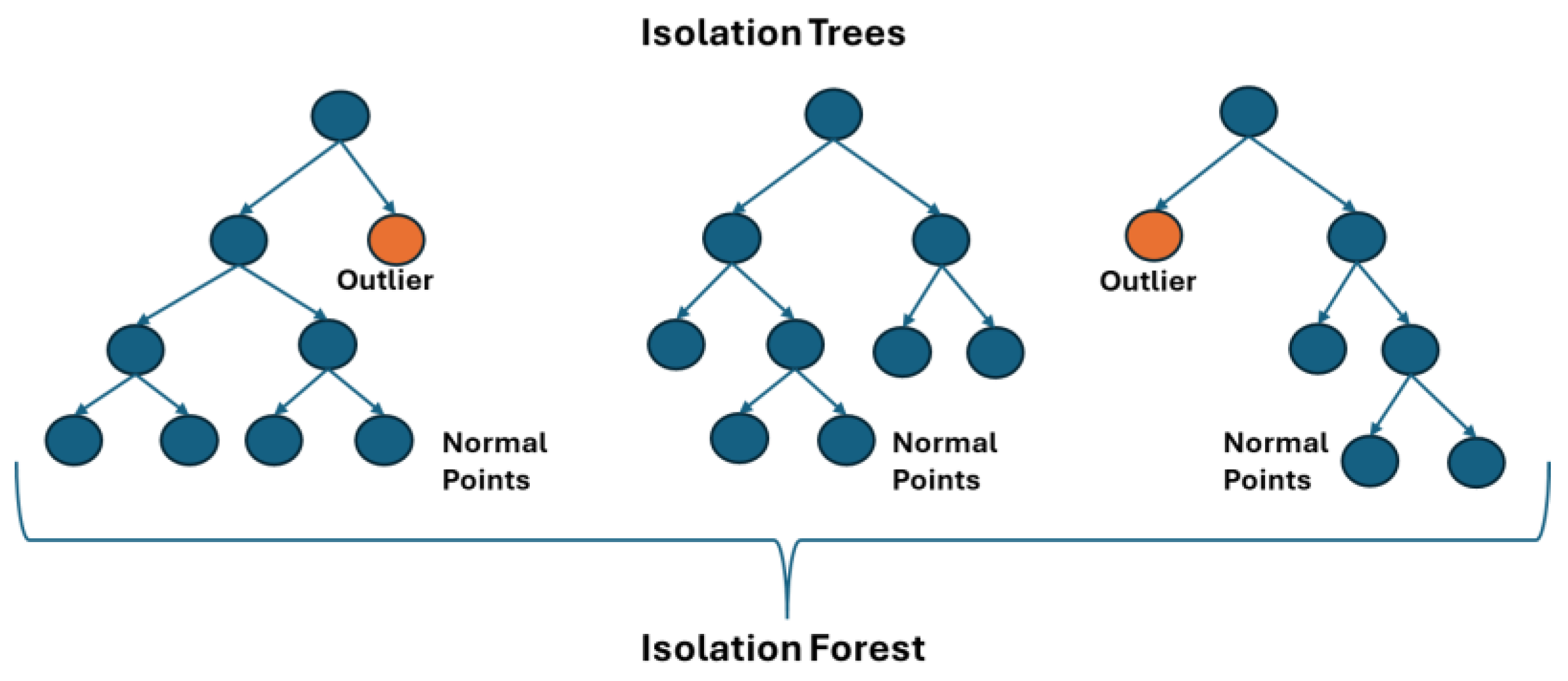
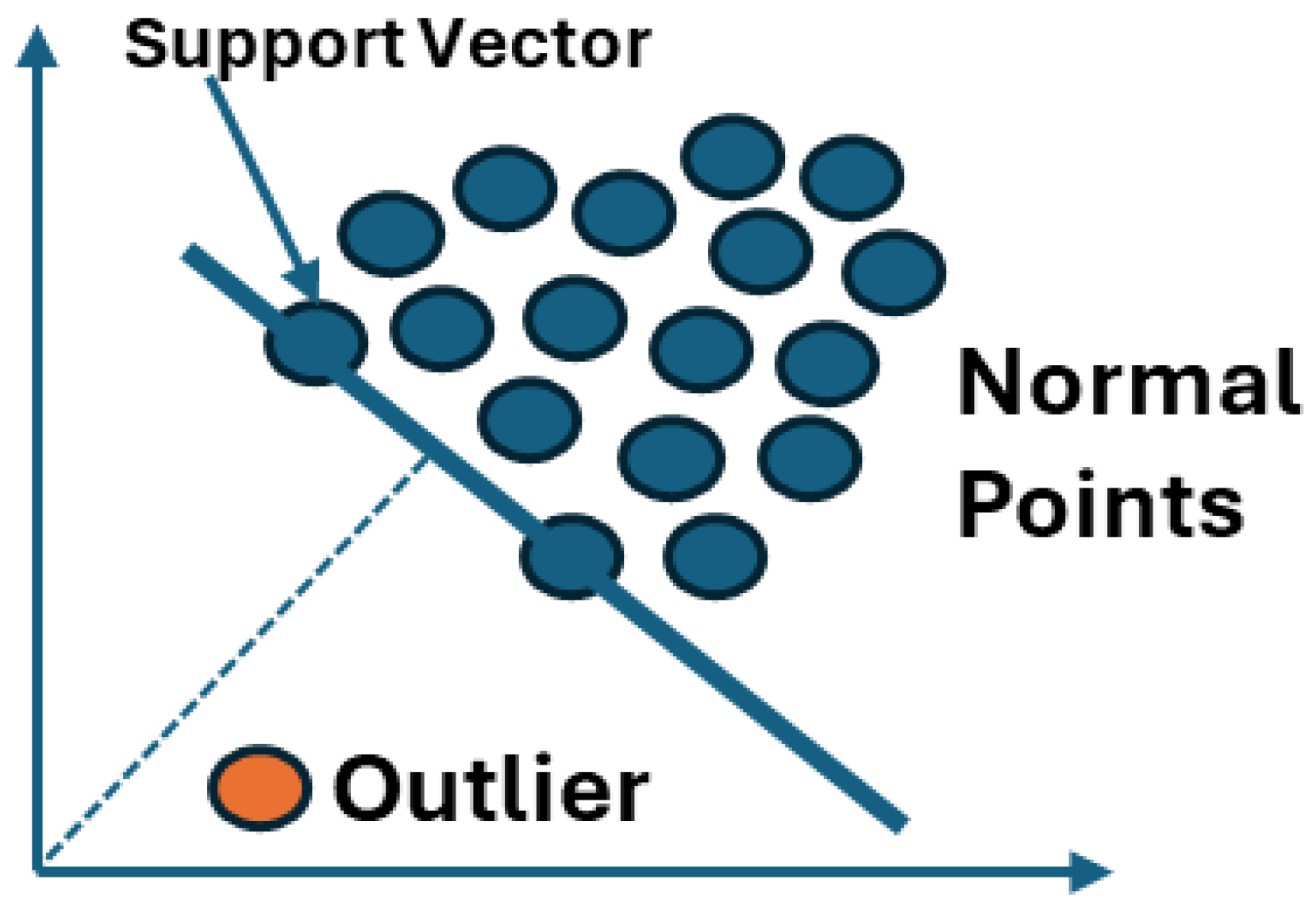
In outlier detection, the goal is to identify and isolate outliers in the data. Outliers can be categorized into Point Outliers and Collective Outliers [13]. In the first category, a single point in a dataset deviates from the rest, while in the second one, there is a collection of points that deviate from the rest of the dataset. For fault detection and severity estimation of a PMSM, the Collective Outlier case is considered, as with the occurrence of a fault, samples that deviate from the normal operation will appear, especially with increasing severity. Three different widely used methods for outlier detection are investigated in this work. The first one is Isolation Forest, proposed by Liu et al. in [14]. The second one is One Class Support Vector Machine (SVM) [15] and the last one is Robust Covariance Ellipse [16]. The three methods are investigated separately and then an ensemble approach is proposed to address the methods’ limitations and further PMSM fault diagnosis challenges.
Several challenges exist in the integration of AI and machine learning for outlier detection and fault diagnosis of electrical machines, and particularly for PMSM. A key challenge is related to the Signal Processing and Feature Extraction stage [17]. The features to be used by the diagnostic model must reflect as close as possible the existence of faults. In addition, they must be as independent as possible of load and speed operating conditions. For this reason, this paper proposes the utilization of the Park transform and the transformation of currents in the d-q rotational reference system. The presence of a fault in the motor leads to the distortion of d-q current signals in both time and frequency domains, so statistical indicators are used to describe these changes. An additional challenge in diagnosing PMSM faults has to do with the estimation of the severity of the fault. Other than the prediction of a fault, the diagnostic system should also give an estimate of how serious it is for the appropriate action to be taken. For this reason, the so-called Anomaly or Outlier Scores extracted by the selected methods are exploited. Moreover, for a specific diagnostic task, many models may fit and perform well, so a combination of them may yield to better results, improving the overall performance of the diagnostic system. For this reason, simple ensemble approaches, like Majority Voting and Mean Ensemble [18], which combine independently the predictions and scores from the used models, are employed.

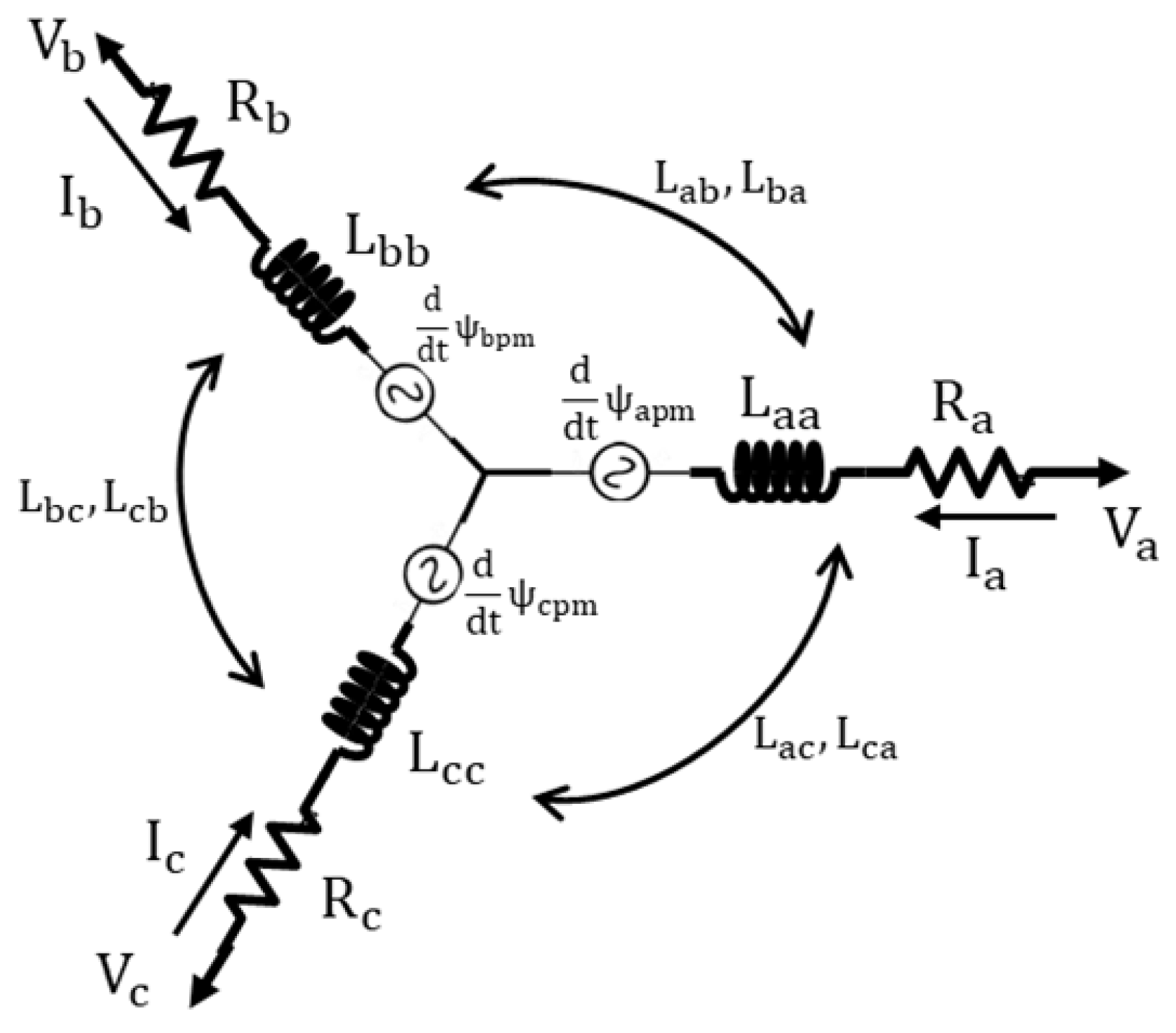
2. PMSM Mathematical Model

The voltage equations of the PMSM in the abc reference system are the following:
V a t V b t V c t = R s 0 0 0 R s 0 0 0 R s · I a t I b t I c t + d ψ a t d t d ψ b t d t d ψ c t d t
where R s is the stator’s winding resistance, I a ,     I b , I c are the stator’s phase currents, and ψ a ,   ψ b ,   ψ c are the stator’s flux linkages, which are given by the following equations:
ψ a t ψ b t ψ c t = L a a L a b L a c L b a L b b L b c L c a L c b L c c · I a t I b t I c t + ψ a p m t ψ b p m t ψ c p m t
where L x x is the self-inductance of the x phase, L x y is the mutual inductance of the x and y phases, and ψ a p m , ψ b p m ,   ψ c p m are the flux linkages associated to the windings abc and the permanent magnets. A schematic representation of the PMSM model is shown in Figure 1.
To simplify the above equations, the Park transform is used, where the Park matrix is obtained as:
T θ = 2 3   sin θ sin θ 2 π 3 sin θ + 2 π 3 cos θ cos θ 2 π 3 cos θ + 2 π 3 0.5 0.5 0.5
with respect to an arbitrary reference frame with reference angle θ and q-axis alignment. By selecting θ = θ e , where θ e is the rotational reference angle, the simplified voltage equations are the following:
V q = R s I q + L q d I q d t + p ω I d L d + ψ p m V d = R s I d + L d d I q d t p ω I q L q
where p is the number of pole pairs, L q , L d are the d-q reference frame inductances, ψ p m is the flux linkage associated with permanent magnets. The zero sequence Vo is neglected here.

3. Motor d-q Current Signature Analysis

Motor Current Signature Analysis (MCSA) relies on examining a motor’s stator current to find specific patterns associated with faults. The stator’s current is analyzed in the frequency domain in the interest of extracting specific frequencies associated with motor’s faults. For a healthy motor, the form of stator currents is as follows:
I A h t = A s i n 2 π f s t I B h t = A s i n 2 π f s t 2 π 3 I C h t = A s i n 2 π f s t + 2 π 3
Using the Park transform matrix in the synchronous rotational reference system ( θ = θ e ) :
I q I d = 2 3 cos θ e cos θ e 2 π 3 cos θ e + 2 π 3 sin θ e sin θ e 2 π 3 sin θ e + 2 π 3 · I a I b I c
It follows that:
I q h = A 3 I d h = 0
With the presence of a fault in the motor, additional harmonics appear in the current’s spectrum. The frequency patterns for MCSA related to eccentricity, demagnetization, and bearings faults are presented in Table 1.
Currents under faulty PMSM state can be expressed as follows:
I A t = A s i n 2 π f s t + κ A κ sin 2 π f k t = I A h t + I A f ( t ) I B t = A s i n 2 π f s t 2 π 3 + κ A κ sin 2 π f k t 2 π 3 = I B h t + I B f ( t ) I c t = A s i n 2 π f s t + 2 π 3 + κ A κ sin 2 π f k t + 2 π 3 = I C h t + I C f ( t )
The above-mentioned quantities are expressed in the synchronous rotational reference system as:
I q = I q h + I q f = A 3 + I q f I d = I d h + I d f = I d f
From the above equations, we can observe that currents in the d-q rotating system contain two quantities, the dc quantities I q h , I d h , which refer to the healthy operational state, and the oscillating quantities I q f ,     I d f , which refer to additional harmonics associated with the fault. By analyzing the above quantities in the frequency domain, the frequencies that occur beyond dc can be used to detect and identify PMSM faults.

4. Features Extraction

To extract useful indicators of fault conditions from d-q currents, multiple features can be exploited. The occurrence of a fault affects both the form of d-q current in time and frequency domains. The fault’s effect on the current’s time waveform can be described by features such as standard deviation, variance, skewness, and kurtosis. In the current spectrum, the appearance of fault harmonics results in the distortion of the shape with the appearance of new peaks. Depending on the fault and its severity, the amplitudes and position of the harmonics may vary. To describe the spectrum, various spectral descriptors can be used. The spectral features shown in Table 2 are used for this task. It is important to note that the total features to be used should be kept as few as possible so that computational complexity remains low, but they must also be sufficient to describe the desired fault characteristics.

5. Outlier Detection

5.1. Isolation Forest (iForest)

Isolation Forest (iForest) is an unsupervised outlier detection method that was proposed by Liu et al. [14]. iForest creates a forest of decision trees and assigns anomaly scores to every data point in the forest according to the length from the root node. The basic idea is to assign high anomaly scores to the data points with the least length and thus identify outliers.
iForest consists of two phases, the training and evaluating phases. Considering a dataset X with n samples and m features, training starts by selecting a subset of data and building the first Isolation Tree. The procedure is repeated until a certain number of Isolation Trees are built. Every tree is built by splitting the selected samples. Splitting is performed by randomly selecting a feature and a value between the maximum and minimum value of the selected feature. The splitting procedure is repeated until a certain depth in the tree is achieved. In the second phase, the evaluating phase, each data point receives a score based on its position in the created forest. The score of every data point is calculated as:
s ( x , n ) = 2 E h x c n
The path of every sample from the root node is denoted as h ( x ) and the average value of the paths from the forest as E h x . By using BST [14], the non-successful search length is computed, which is denoted as c ( n ) . An illustration of the Isolation Forest is shown in Figure 2. Outliers are defined based on shorter paths from the root node of the created Isolation Trees.

5.2. One-Class SVM

Support Vector Machines (SVMs) are a class of supervised machine learning methods that are used in a variety of applications for classification. The basic idea behind SVM is to find an optimal hyperplane to separate the data. Linear SVM is used to find an optimal ‘maximum-margin’ hyperplane to separate data. To deal with nonlinear classification tasks, kernel tricks are used. Kernels are used to map the data space into a higher-dimensional space, the feature space, where classification can be achieved. The functions that are used more as kernels are polynomial, radial basis function (rbf), and sigmoid.
One Class Support Vector Machines (One Class SVMs) have been proposed for novelty and outlier detection [15]. The goal is to find a function that separates the data from the origin through separating normal data in a specific region. Data points outside that region can be considered anomalies. Consider a dataset X with n samples and m features, Φ, a feature mapping from data space X to feature space F, and a kernel:
k ( x , y ) = ( Φ x · Φ ( y ) )
The quadratic problem to be solved in the case of One Class SVM is the following:
min 1 2 | | w | | 2 + 1 v · m i ξ i ρ
subject to:
w   · Φ x i ρ ξ i ,   ξ i 0
where w , ρ are the weight and bias terms of the hyperplane, ξ i are the slack variables, and v is an adjustable parameter.
The dual-Lagrangian problem is derived as:
min a 1 2 i j a i a j k ( x i . y i )
Solving the above problem, the coefficients of the following decision function are derived:
f x = s i g n i a i k x i ,   x ρ
In Equation (12), the parameter v ( 0,1 ) is used in the second term to adjust the slack variables’ effect on the quadratic problem. The parameter controls the trade-off between the number of outliers and the margin from the origin. If v 0 , then the boundaries of the hyperplane are loose, and then it separates all data from the origin. If v 1 , then the boundaries of the hyperplane become tighter, and it separates less data from the origin. An illustration of One Class SVM is shown in Figure 3.

5.3. Robust Covariance Ellipse

For a dataset X with n samples and m features, the Mahalanobis distance is given as:
M D x = x x ¯ T S 1 ( x x ¯ )
where x ¯ is the mean, S is the covariance matrix of the samples, and T is the annotation of the transpose operation. The calculated distance of every data point can be used to define a region of normal data and outliers. In the calculation of mean and covariance, outliers can affect the calculated values, thus leading to the identification of outliers as normal data, an effect also known as the ‘Masking Effect’ [16]. To enhance robustness against this effect, Minimum Covariance Determinant (MCD) is used to estimate the mean and the covariance matrix. The MCD computes the mean and the covariance matrix for h observations, where h > m and can be calculated as h = n + m + 1 2 . FAST-MCD [19] is employed for MCD implementation due to computation speed and efficiency. After the estimation of robust mean and covariance, the Mahalanobis distance for every sample is calculated. An illustration of the computed Robust Covariance Ellipse is shown in Figure 4.

5.4. Outlier Ensemble Approach

Outlier ensembles have been quite categorized in [16]. Depending on the structure of the ensemble, Sequential and Independent Ensemble or Model-Centered and Data-Centered Ensembles can be employed [20]. The approach used in this work falls into Independent and Model-Centered categories, where the whole dataset is used from all the outlier detection models, as shown in Figure 5. Each model generates anomaly scores for each sample point. The use of scores from multiple different models may require normalization as each model generates different arithmetic values. Averaging Ensemble can be used to extract averaging anomaly scores and can be carried out by simply averaging the values of each model. Weighted Averaging can also be employed, where values of each model are multiplied by a certain weight to place emphasis on certain values. Typical weights include statistical, adaptive, or case-specific ones [18]. Instead of Averaging, Max or RMS value of the overall normalized scores for each sample point can also be used. Like Scores Ensemble, Average, Max, and RMS value of predictions from each model can be employed. Majority Voting can also be used, where the majority of predictions are selected. Various approaches are assessed and compared through experimental tests in Section 6.

6. Experimental Procedure and Results

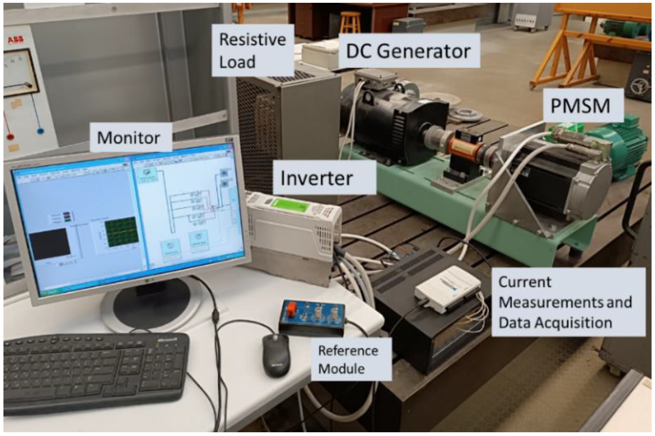
The test bench that was used for the experimental procedure is shown in Figure 6. The test rig consists of a Nidec’s (Sycracuse, NY, USA) PMSM and DC Generator, a resistive load, an Inverter, a Current Measurement Unit, a Data Acquisition Unit, and a PC. The PMSM is coupled to the DC Generator through a flexible coupling. The DC Generator with the resistive load is used as a load for the PMSM. The PMSM parameters are shown in Table 3.
The acquisition of current measurements is performed with a sampling frequency of 5 kHz using an NI Daq and LABVIEW. The fault considered in this case is a misalignment between PMSM and the DC Generator, causing eccentricity effects in the PMSM’s shaft. It was achieved by placing metal shims in the support base of the motor. Two levels of fault severity were considered by different shim widths.
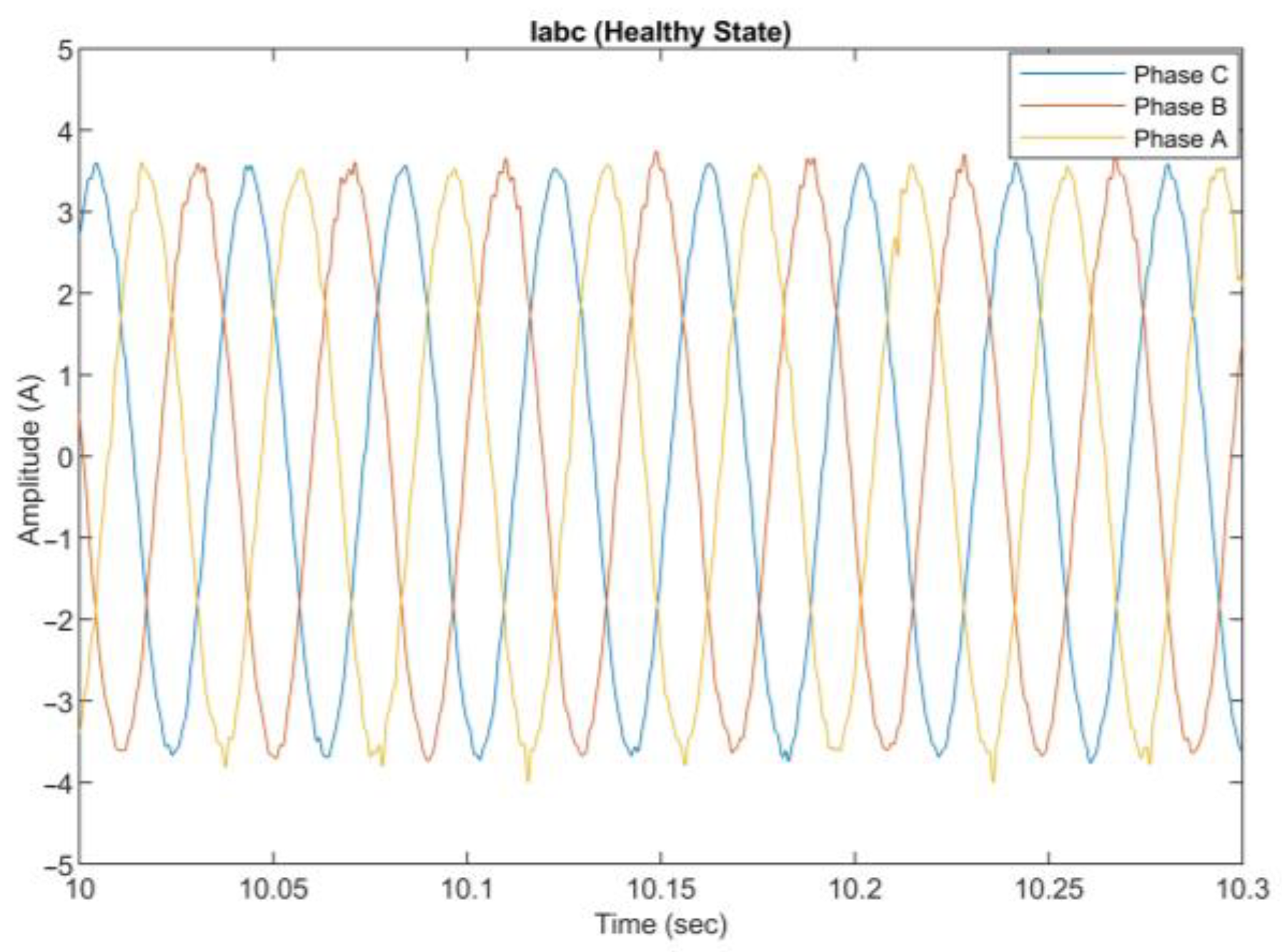
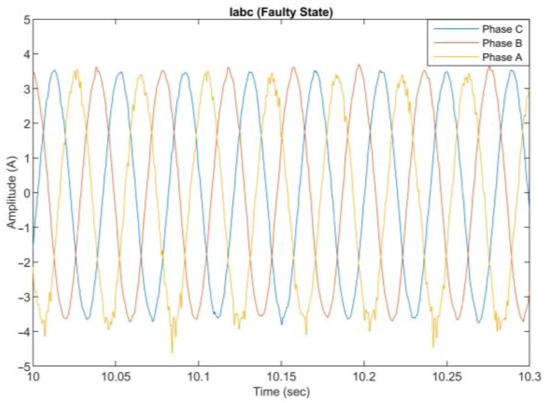
The collected data consist of three-phase current measurements for healthy and faulty operating conditions with increasing severity. In Figure 7 and 
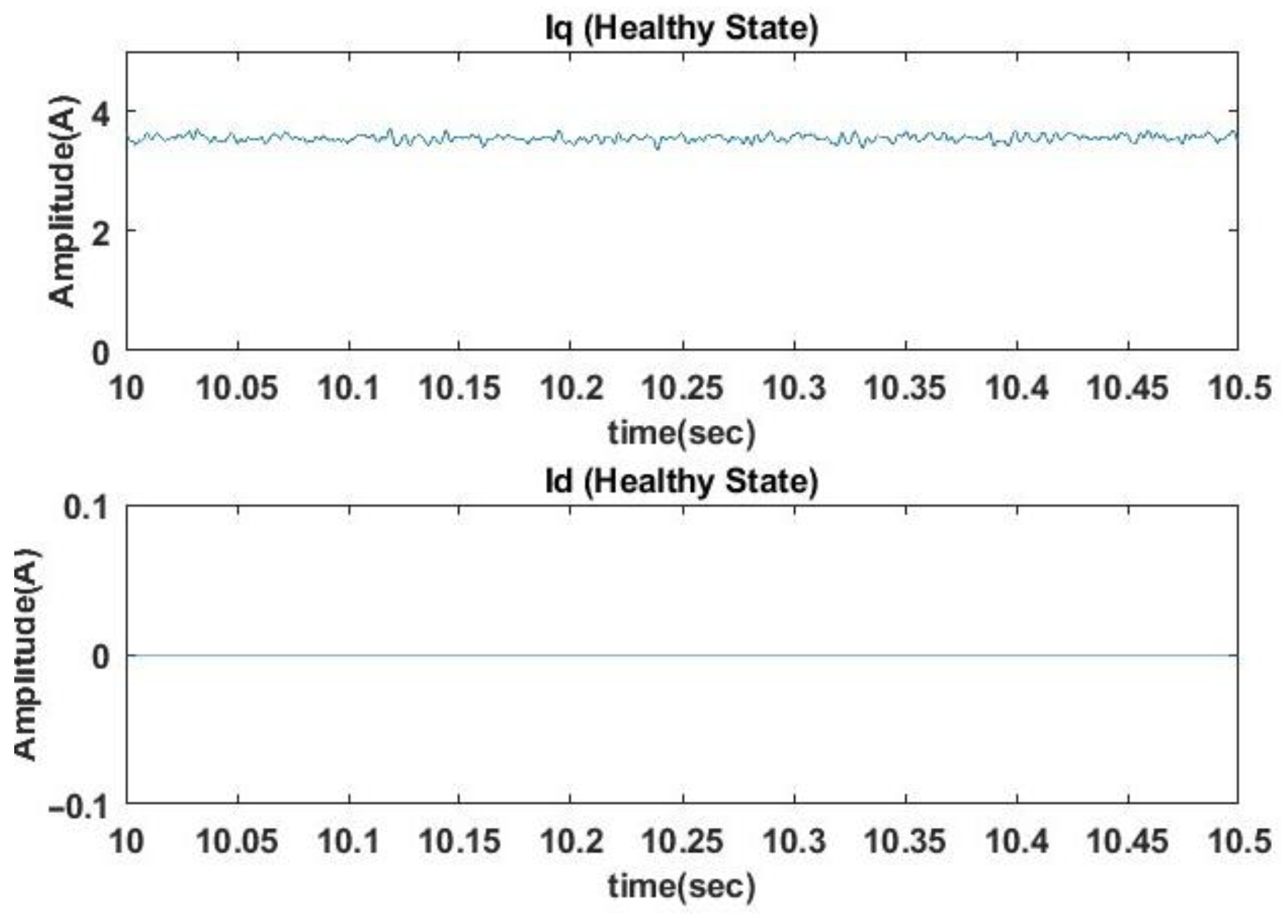
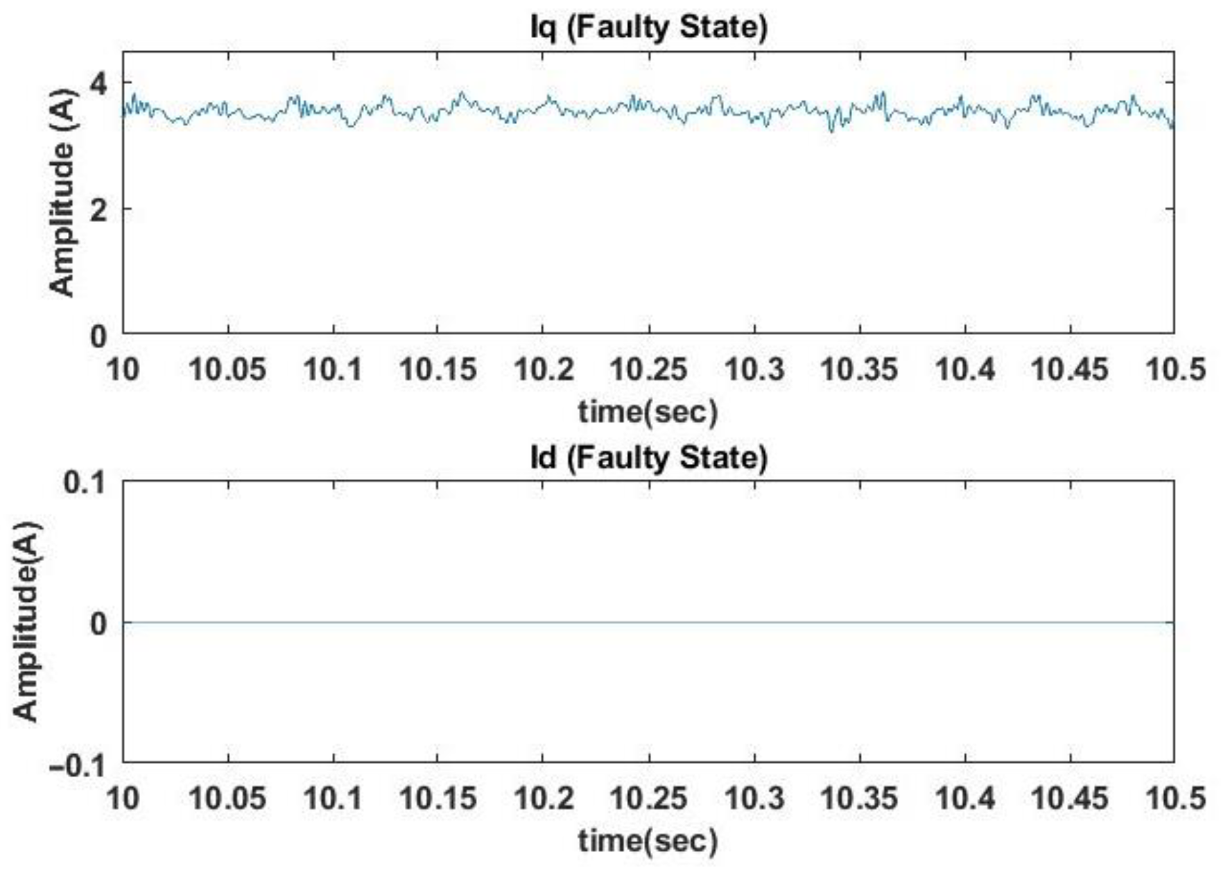
Figure 8, abc current time waveforms for healthy and faulty operating conditions are presented, respectively. The operating speed of the PMSM is 1400 rpm, with a load of 6 Nm. We can notice the deformation of the waveform’s envelope in the faulty state due to the misalignment. To extract useful features of the faulty conditions, such as time and frequency domain features, d-q transformation and FFT analysis are employed. In Figure 9 and Figure 10, the corresponding waveforms for q and d axis current in a rotating reference frame are presented. The d current waveform remains at zero, as Field Oriented Control (FOC) is used to drive the PMSM. We observe an increased ripple and distortion in q current signal over time, due to the additional harmonics caused by the misalignment condition.
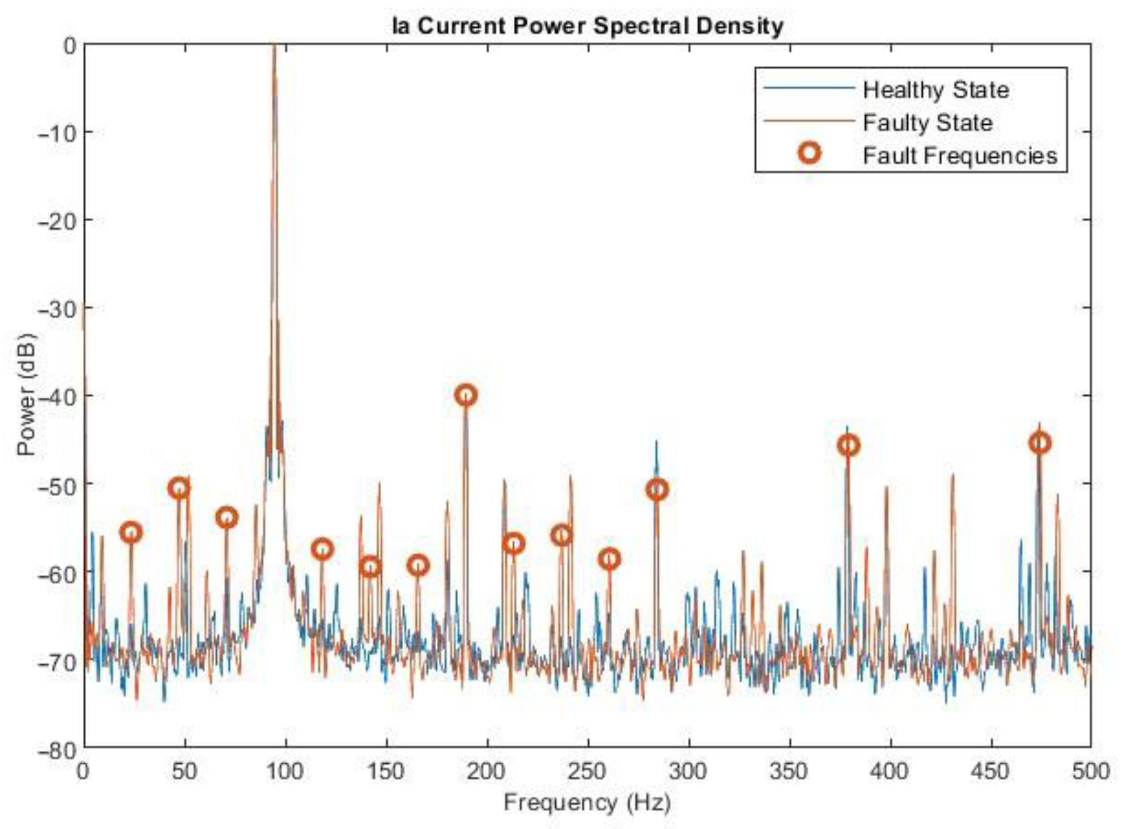
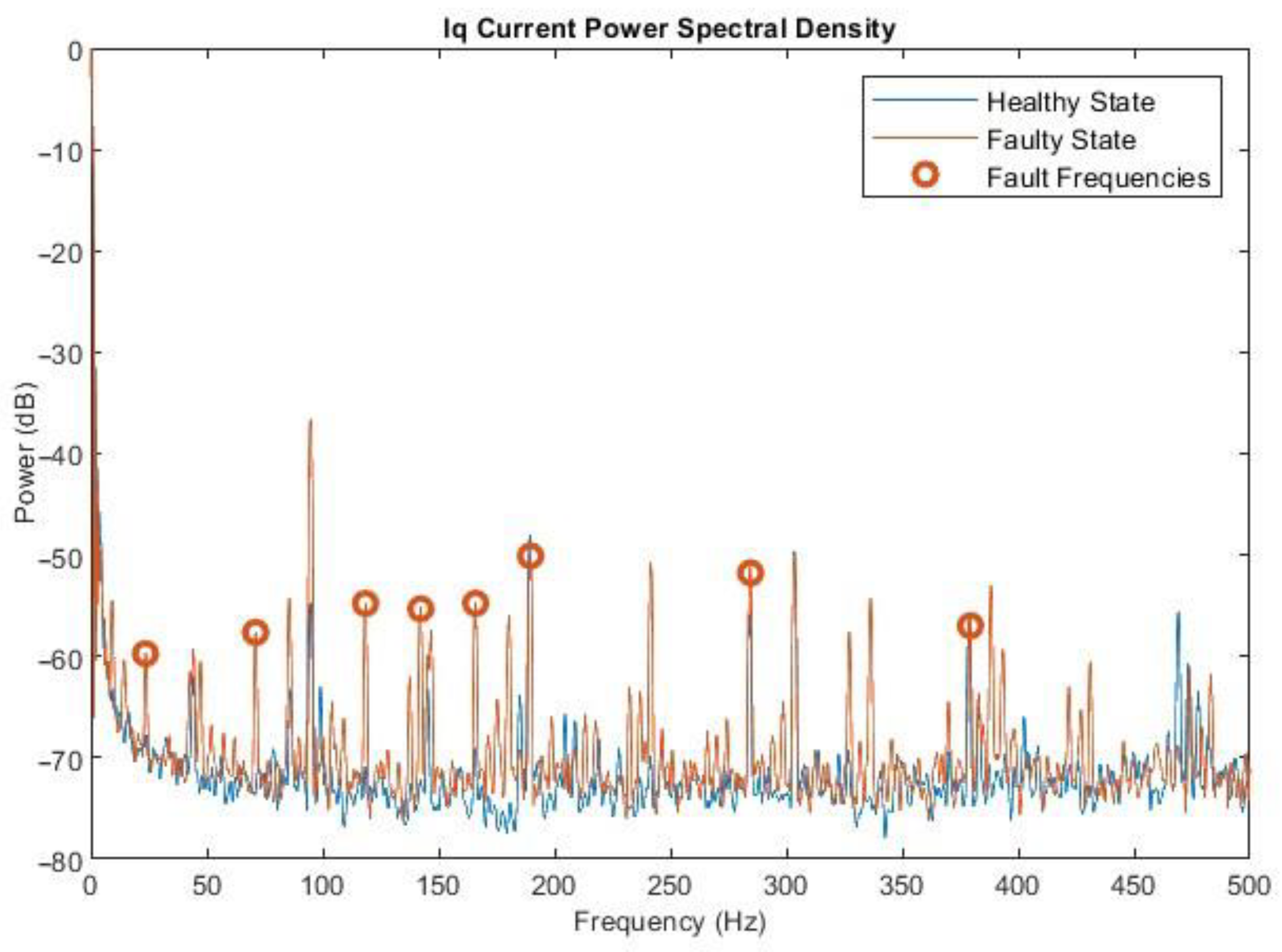
To derive the frequency characteristics of the fault, analysis of the current in the frequency domain is required. For this reason, in Figure 11 and Figure 12, Power Spectral Density is calculated. In Figure 11, the spectrum of the healthy state (blue color) and faulty state (red color) are placed together. The specific eccentricity-related fault harmonics are indicated with red circles. In Figure 11, the q-axis Power Spectral Density is shown for the same conditions. Due to design and operation parameters of the PMSM test bench, some harmonics that follow the eccentricity-related pattern are also evident in the healthy state.
From the waveform of the current over time, the statistical features of standard deviation, variance, skewness, and kurtosis are calculated, and from the signal’s power spectrum, spectral density, spectral centroid, spectral spread, spectral skewness, and spectral kurtosis indices are calculated. The above characteristics are calculated for four different speeds and four different load levels under a healthy and faulty (misalignment) condition. The overall dataset consists of the above features for different operating modes and with an increasing severity of the fault.
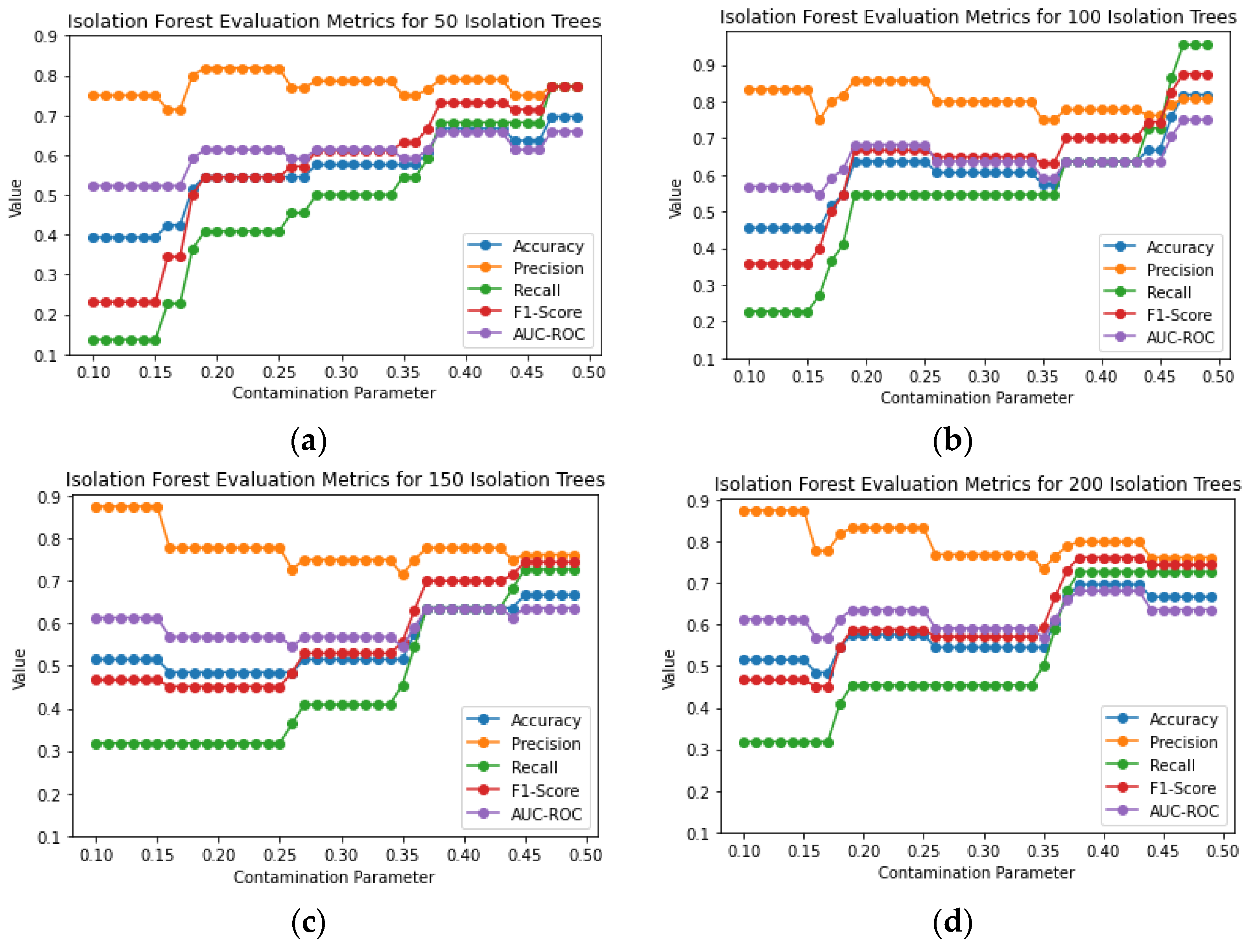
Initially, we investigate the three different methods separately and compare them. The implementation of all methods is performed using Python and Scikit-learn. First, the Isolation Forest is investigated. The training of the model is performed with healthy data, while the test is performed with a dataset of healthy data and faulty data with increasing severity of the misalignment fault. The model’s performance is investigated for different contamination parameter values and number of trees. As the number of samples and features is small in this dataset, the number of maximum features and maximum samples that can be adjusted as parameters are kept to the default values. However, it is important to note that in larger datasets and features, the above two parameters are important, as they can reduce computational complexity and indicate redundant features. Below, in Figure 13 are the evaluation metrics for different values of the contamination parameter and different number of trees. We observe that in all cases (50, 100, 150, 200 iTrees), better evaluation metric values appear in the range of 0.4–0.5 for the contamination parameter. The best evaluation metric values for 100 Isolation Trees and contamination parameter in the range of 0.4–0.5 are shown in Table 4.
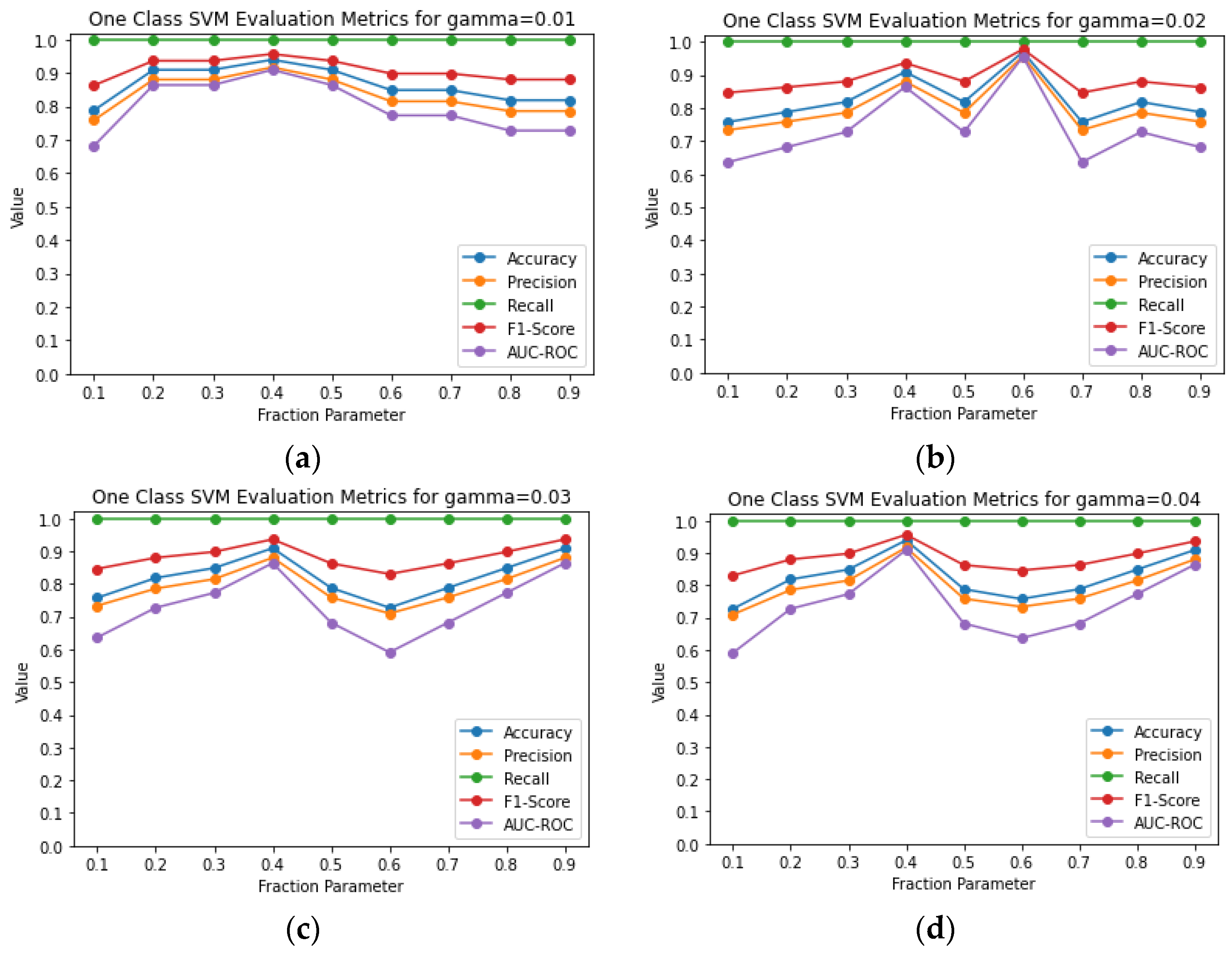
Subsequently, One Class SVM is investigated. Like iForest, only healthy data were used to train the model and then tested with a dataset of healthy and faulty states with increasing severity. One Class SVM was tested for the Radial Basis Function kernel for different gamma and fraction parameter values. The gamma range of the test is between 0.005 and 0.04, as there are no further improvements in the performance of the model above 0.04. This can be seen in the corresponding figures for gamma = 0.02, 0.03, and 0.04, in Figure 14. The best values of evaluation metrics appear for gamma = 0.2 and fraction parameter = 0.6. For these cases, the evaluation metrics are shown in Table 5.
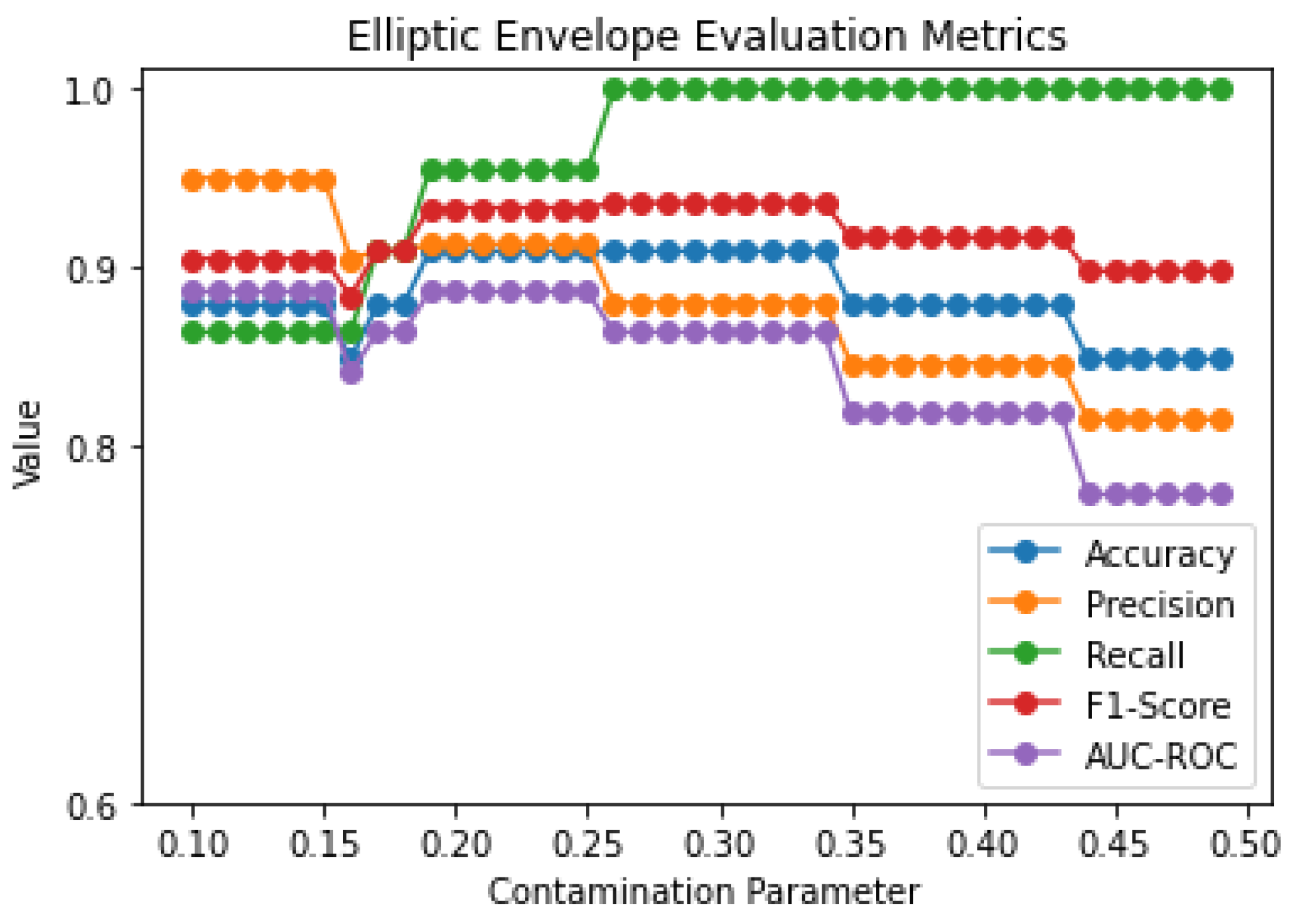
Lastly, Robust Covariance Elliptic Envelope was assessed for the same dataset. The influence of different contamination parameters is shown in Figure 15. We can observe that the best values of the evaluation metrics arise for a contamination parameter equal to 0.2 or 0.3. The evaluation metrics for the above parameters are shown in Table 6. The main difference lies in the decrease in precision and ROC AUC and the increase in Recall and F1-score for contamination parameter equal to 0.2 and 0.3, respectively.
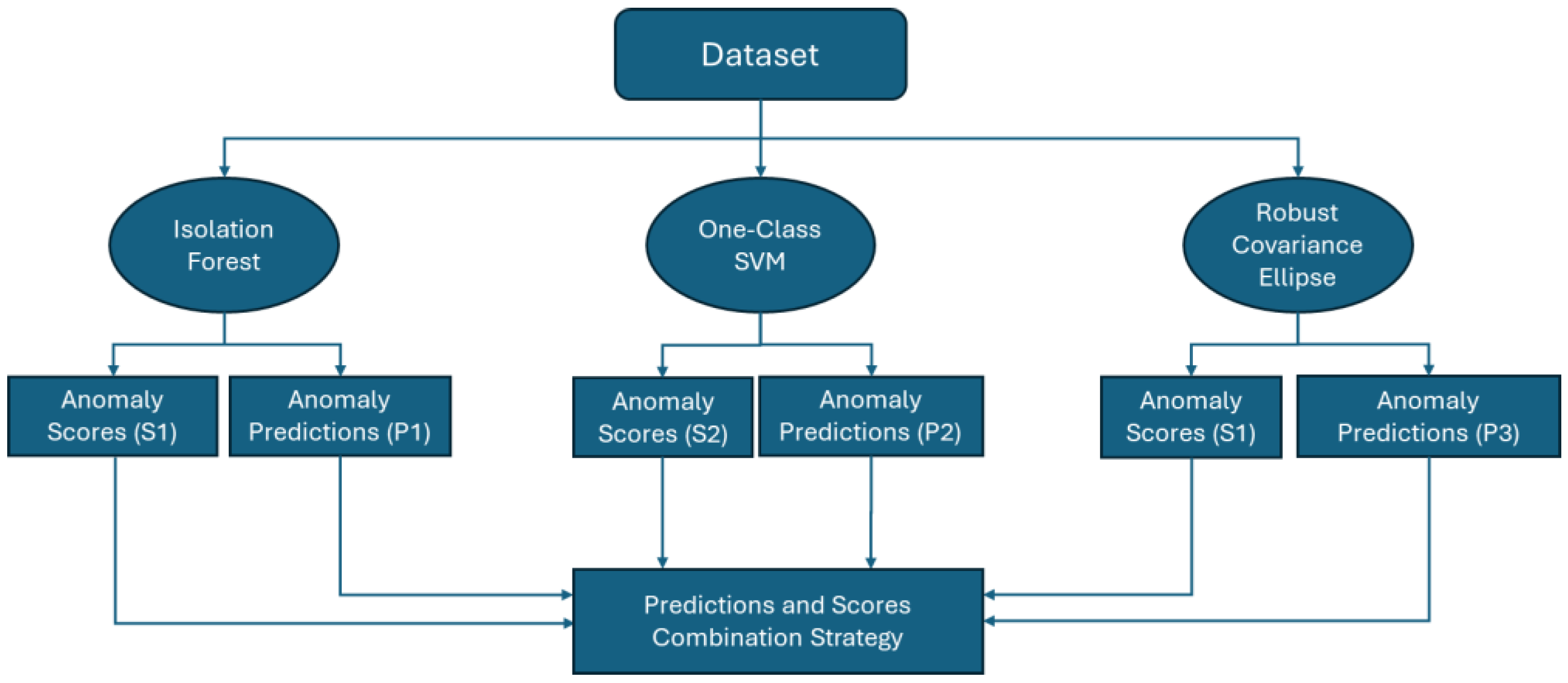
The above models can be combined through different ensemble techniques, as discussed in Section 5. More specifically, Majority Voting Ensemble can be used, where the majority of predictions are selected, and the Average Ensemble, where the average of the predicted values is calculated. Note that in the case of Averaging, rounding of the predicted values is required. The evaluation metrics for the above cases are shown in Table 7.
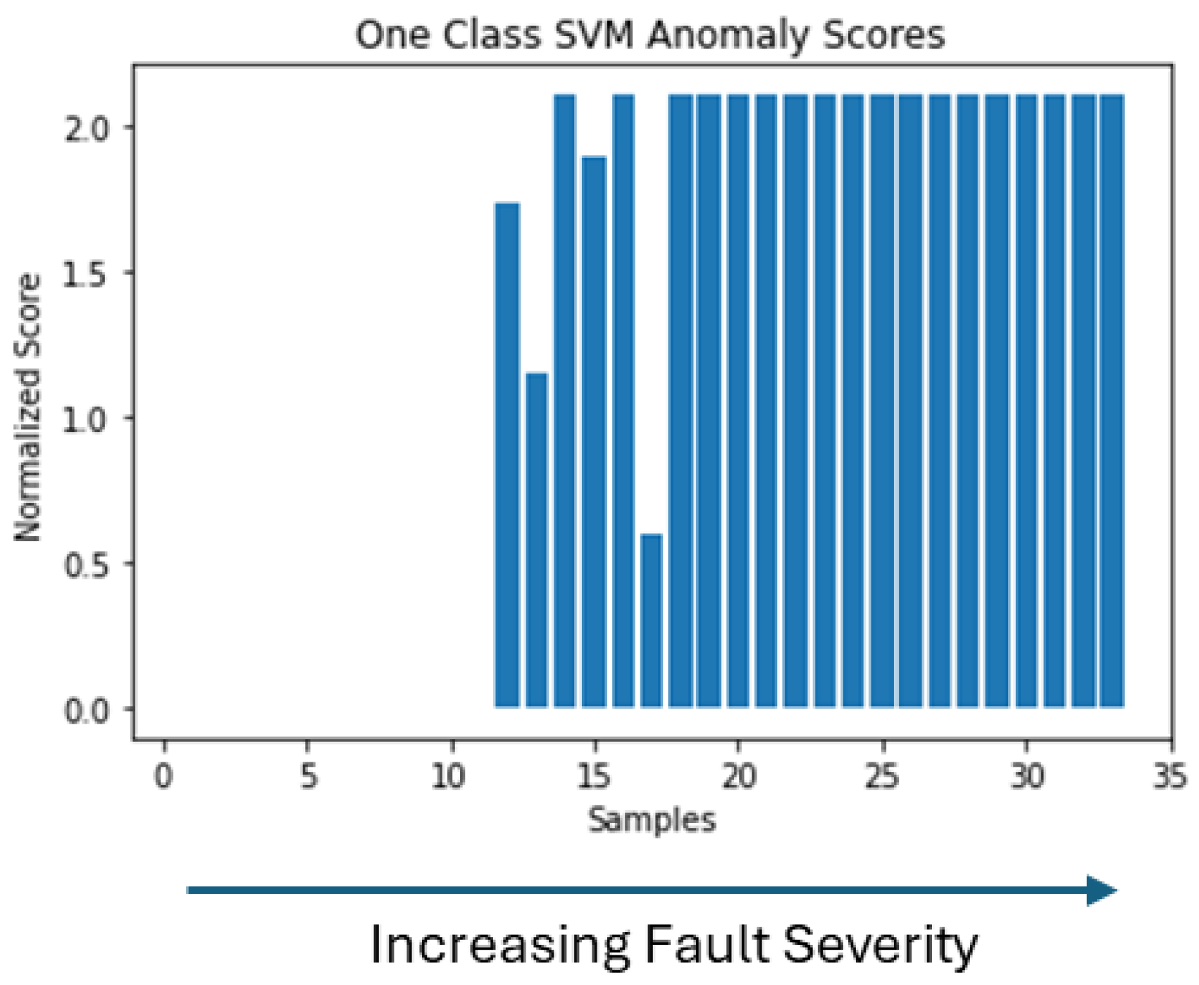
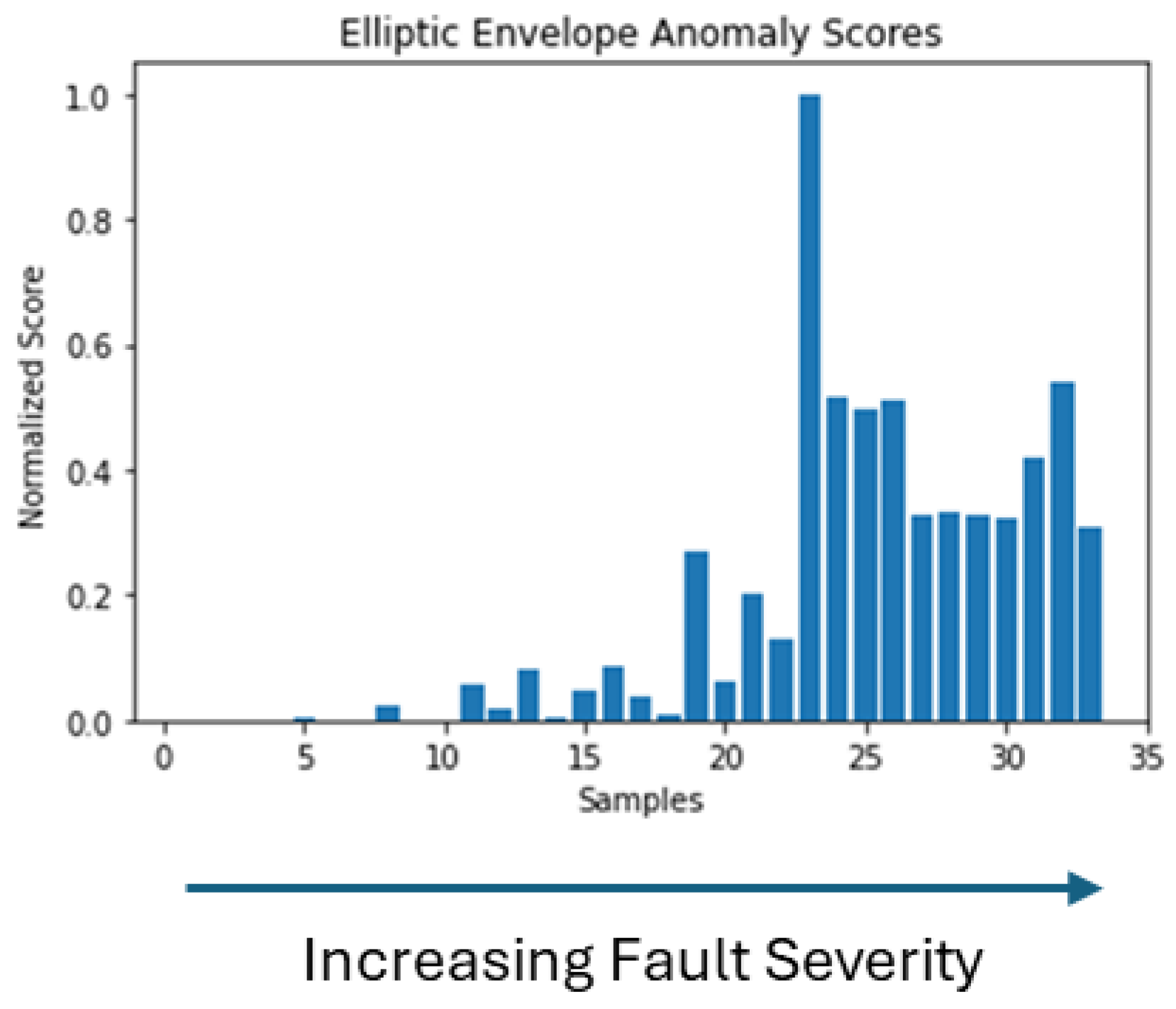
To estimate the severity of the fault, the anomaly scores generated by each model are employed. Based on how anomaly scores are generated, each of the above methods generates a different range of values. For this reason, the values are normalized. Higher anomaly scores indicate faulty operating conditions in the PMSM. In the test dataset, the first 11 samples respond to a healthy working state, while the following 11 respond to a faulty state with a low fault severity, and then the last 11 respond to an increased fault severity. In the case of the One Class SVM, in Figure 16, we can see that healthy samples are distinguished from faulty samples, and especially the latest samples of increased severity. However, the difference between each sample for the latest samples and the increased severity is not clear. In the case of the Isolation Forest, in 
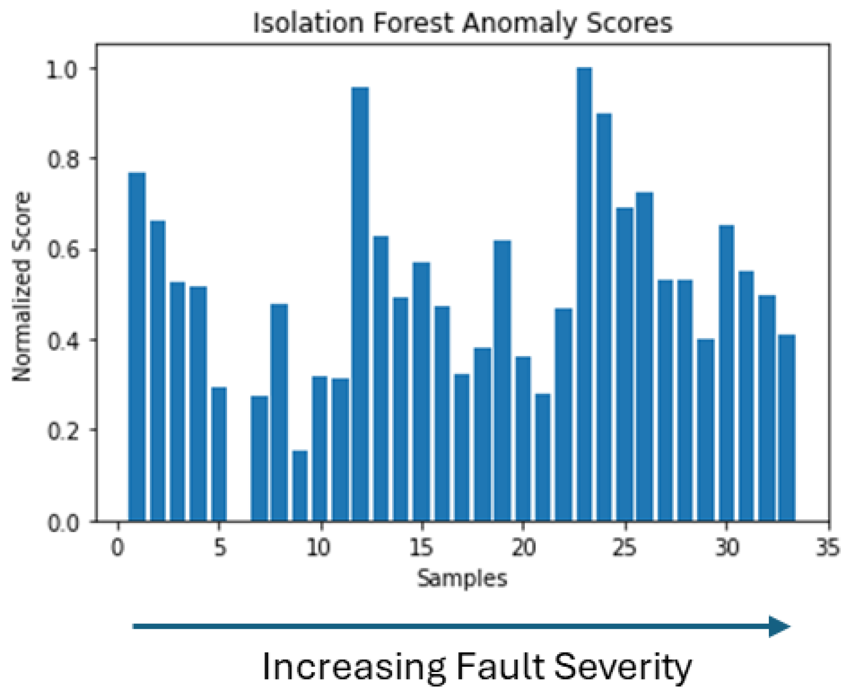
Figure 17, we see that we have increased anomaly scores for faulty cases that can be used as indicators of fault occurrence and increase in severity. In the case of the Elliptic Envelope, in Figure 18, we have the clearest picture, as we observe that anomaly scores are low for healthy samples while increasing with the appearance of the fault and especially at higher severity.
Ensemble techniques can be employed to utilize the scores generated from the models and improve severity estimation. For each sample of the three models, the average values are calculated. This results in the mean anomaly scores, shown in Figure 19. The evaluation metrics extracted in the previous section can be used to introduce weights to each anomaly score produced by each model, respectively. However, in this case, there was no notable change from the mean ensemble, so it was not examined further. Other than Mean Ensemble, Max Ensemble can be employed, where the max values from each model are used. The corresponding anomaly scores are shown in Figure 20.
An additional important piece of information from the generated anomaly scores is related to the detection of conditions where the fault is more intense or detectable. It is known [4,6] that the operating conditions of motor speed and load affect the occurrence and detectability of the fault. By using anomaly scores, we can see in which operating condition the highest anomaly score is displayed, as well as compare each operating condition with the corresponding one with a fault.

7. Conclusions

The proposed methodology utilizes PMSM’s three-phase currents and speed measurements for online, non-invasive, and cost-effective condition monitoring of the PMSM. To extract fault-related features from the measurements, d-q transform was used. Distortions in time waveforms and several eccentricity-related frequencies in the power spectral density were observed for different speed and load conditions of the PMSM. Then, to extract useful indicators of fault conditions, statistical measures in time and frequency domain were used. The extracted statistical features were used for outlier detection by means of fault detection and severity estimation through Isolation Forest, One Class Support Vector Machine (SVM), and Robust Covariance Ellipse.
First, Isolation Forest was investigated for different isolation trees and contamination parameters. The best evaluation metrics were extracted for 100 Isolation Trees and a contamination parameter in the range of 0.4–0.5. The accuracy of Isolation Forest reached 0.82. One Class SVM was employed for the same task. Radial Basis Function was selected as the kernel and different gamma and fraction parameters were investigated. The best evaluation metrics were extracted for gamma equal to 0.2 and fraction parameter equal to 0.6. The accuracy reached 0.97. Lastly, Robust Covariance Ellipse fitting was tested. The highest accuracy achieved was 0.91 for gamma and contamination parameters equal to 0.2 and 0.3, respectively. One Class SVM was the best candidate in terms of Accuracy, Recall, Precision, F1-Score, and ROC AUC. For Severity Estimation, the extracted Outlier Anomaly Scores from the above methods were used. Comparing the three methods, increasing fault severity was better observed in Outlier Scores generated by Robust Covariance Ellipse fitting, then Isolation Forest, and lastly, One Class SVM. To combine the predictions and outlier scores, and so the advantages of each method, Independent Ensemble approaches are proposed. Majority Voting and Averaging Ensemble of the predictions led to Accuracy equal to 0,94 and 0,97, respectively. Max and Mean Ensemble of the Outlier Scores led to better observability of the increasing severity by each sample of the tested dataset.

Author Contributions

Conceptualization, K.K. and E.M.; methodology, K.K.; software, K.K.; validation, K.K., investigation, K.K.; resources, K.K.; data curation, K.K. and E.M.; writing—original draft preparation, K.K and E.M.; writing—review and editing, K.K and E.M.; supervision, E.M.; project administration, E.M. All authors have read and agreed to the published version of the manuscript.

Funding

This research received no external funding.

Institutional Review Board Statement

Not applicable.

Informed Consent Statement

Not applicable.

Data Availability Statement

The raw data supporting the conclusions of this article will be made available by the authors on request.

Acknowledgments

The present work was financially supported by the “Andreas Mentzelopoulos Foundation” (Corresponding Author: K.K.).

Conflicts of Interest

The authors declare no conflicts of interest.

References

  1. Koutrakos, K.; Mitronikas, E. Detection of Shaft Misalignment of a PMSM using Zoom-FFT. In Proceedings of the 2023 IEEE 14th International Symposium on Diagnostics for Electrical Machines, Power Electronics and Drives (SDEMPED), Chania, Greece, 28–31 August 2023; pp. 96–102. [Google Scholar] [CrossRef]
  2. Rosero, J.; Romeral, J.L.; Cusido, J.; Ortega, J.A.; Garcia, A. Fault detection of eccentricity and bearing damage in a PMSM by means of wavelet transforms decomposition of the stator current. In Proceedings of the 2008 Twenty-Third Annual IEEE Applied Power Electronics Conference and Exposition, Austin, TX, USA, 24–28 February 2008; pp. 111–116. [Google Scholar] [CrossRef]
  3. Lamprokostopoulos, A.; Mitronikas, E.; Barmpatza, A. Detection of Demagnetization Faults in Axial Flux Permanent-Magnet Synchronous Wind Generators. Energies 2022, 15, 3220. [Google Scholar] [CrossRef]
  4. Qi, Y.; Bostanci, E.; Gurusamy, V.; Akin, B. A Comprehensive Analysis of Short-Circuit Current Behavior in PMSM Interturn Short-Circuit Faults. IEEE Trans. Power Electron. 2018, 33, 10784–10793. [Google Scholar] [CrossRef]
  5. Osmani, K.; Haddad, A.; Lemenand, T.; Castanier, B.; Alkhedher, M.; Ramadan, M. A critical review of PV systems’ faults with the relevant detection methods. Energy Nexus 2023, 12, 100257. [Google Scholar] [CrossRef]
  6. Niu, G.; Dong, X.; Chen, Y. Motor Fault Diagnostics Based on Current Signatures: A Review. IEEE Trans. Instrum. Meas. 2022, 72, 3520919. [Google Scholar] [CrossRef]
  7. Henao, H.; Capolino, G.-A.; Fernandez-Cabanas, M.; Filippetti, F.; Bruzzese, C.; Strangas, E.; Pusca, R.; Estima, J.; Riera-Guasp, M.; Hedayati-Kia, S. Trends in Fault Diagnosis for Electrical Machines: A Review of Diagnostic Techniques. IEEE Ind. Electron. Mag. 2014, 8, 31–42. [Google Scholar] [CrossRef]
  8. Orlowska-Kowalska, T.; Wolkiewicz, M.; Pietrzak, P.; Skowron, M.; Ewert, P.; Tarchala, G.; Krzysztofiak, M.; Kowalski, C.T. Fault Diagnosis and Fault-Tolerant Control of PMSM Drives–State of the Art and Future Challenges. IEEE Access 2022, 10, 59979–60024. [Google Scholar] [CrossRef]
  9. Ebrahimi, B.M.; Roshtkhari, M.J.; Faiz, J.; Khatami, S.V. Advanced Eccentricity Fault Recognition in Permanent Magnet Synchronous Motors Using Stator Current Signature Analysis. IEEE Trans. Ind. Electron. 2014, 61, 2041–2052. [Google Scholar] [CrossRef]
  10. Cai, B.; Zhao, Y.; Liu, H.; Xie, M. A Data-Driven Fault Diagnosis Methodology in Three-Phase Inverters for PMSM Drive Systems. IEEE Trans. Power Electron. 2017, 32, 5590–5600. [Google Scholar] [CrossRef]
  11. Lee, H.; Jeong, H.; Koo, G.; Ban, J.; Kim, S.W. Attention Recurrent Neural Network-Based Severity Estimation Method for Interturn Short-Circuit Fault in Permanent Magnet Synchronous Machines. IEEE Trans. Ind. Electron. 2021, 68, 3445–3453. [Google Scholar] [CrossRef]
  12. Skowron, M.; Orlowska-Kowalska, T.; Kowalski, C.T. Detection of Permanent Magnet Damage of PMSM Drive Based on Direct Analysis of the Stator Phase Currents Using Convolutional Neural Network. IEEE Trans. Ind. Electron. 2022, 69, 13665–13675. [Google Scholar] [CrossRef]
  13. El-Dalahmeh, M.; Al-Greer, M.; Bashir, I.; El-Dalahmeh, M.; Demirel, A.; Keysan, O. Autonomous fault detection and diagnosis for permanent magnet synchronous motors using combined variational mode decomposition, the Hilbert-Huang transform, and a convolutional neural network. Comput. Electr. Eng. 2023, 110, 108894. [Google Scholar] [CrossRef]
  14. Boukerche, A.; Zheng, L.; Alfandi, O. Outlier Detection: Methods, Models, and Classification. ACM Comput. Surv. 2020, 53, 55. [Google Scholar] [CrossRef]
  15. Liu, F.T.; Ting, K.M.; Zhou, Z.-H. Isolation Forest. In Proceedings of the 2008 Eighth IEEE International Conference on Data Mining, Pisa, Italy, 15–19 December 2008; pp. 413–422. [Google Scholar] [CrossRef]
  16. Shin, H.J.; Eom, D.-H.; Kim, S.-S. One-class support vector machines—An application in machine fault detection and classification. Comput. Ind. Eng. 2005, 48, 395–408. [Google Scholar] [CrossRef]
  17. Márquez-Vera, M.; Ramos-Velasco, L.; López-Ortega, O.; Zúñiga-Peña, N.; Ramos-Fernández, J.; Ortega-Mendoza, R. Inverse fuzzy fault model for fault detection and isolation with least angle regression for variable selection. Comput. Ind. Eng. 2021, 159, 107499. [Google Scholar] [CrossRef]
  18. Hubert, M.; Debruyne, M. Minimum covariance determinant. WIREs Comput. Stat. 2009, 2, 36–43. [Google Scholar] [CrossRef]
  19. Aggarwal, C.C. Outlier Analysis; Springer Science and Business Media LLC: Dordrecht, The Netherlands, 2017. [Google Scholar] [CrossRef]
  20. Mienye, I.D.; Sun, Y. A Survey of Ensemble Learning: Concepts, Algorithms, Applications, and Prospects. IEEE Access 2022, 10, 99129–99149. [Google Scholar] [CrossRef]
Figure 1. PMSM mathematical model.
Applsci 14 04318 g001
Figure 2. Isolation Forest illustration.
Applsci 14 04318 g002
Figure 3. One Class SVM illustration.
Applsci 14 04318 g003
Figure 4. Robust Covariance Ellipse illustration.
Applsci 14 04318 g004
Figure 5. Independent Outlier Ensemble approach.
Applsci 14 04318 g005
Figure 6. Configuration of the PMSM test bench for fault detection and severity estimation.
Applsci 14 04318 g006
Figure 7. Motor ABC current waveforms in healthy state.
Applsci 14 04318 g007
Figure 8. Motor ABC current waveforms in faulty state.
Applsci 14 04318 g008
Figure 9. 3 Motor d-q current waveforms in healthy state.
Applsci 14 04318 g009
Figure 10. Motor d-q current waveforms in faulty state.
Applsci 14 04318 g010
Figure 11. A-phase current Power Spectral Density.
Applsci 14 04318 g011
Figure 12. q-axis current Power Spectral Density.
Applsci 14 04318 g012
Figure 13. Isolation Forest evaluation metrics for 50 (a), 100 (b), 150 (c), 200 (d) Isolation Trees and contamination parameter in the range of 0.1–0.5.
Applsci 14 04318 g013
Figure 14. One Class SVM evaluation metrics for gamma equal to 0.01 (a), 0.02 (b), 0.03 (c), 0.04 (d) and fraction parameter in the range 0.1–0.9.
Applsci 14 04318 g014
Figure 15. Robust Covariance Ellipse evaluation metrics for contamination parameter 0.1–0.5.
Applsci 14 04318 g015
Figure 16. One Class SVM generated anomaly scores.
Applsci 14 04318 g016
Figure 17. Isolation Forest generated anomaly scores.
Applsci 14 04318 g017
Figure 18. Robust Covariance Ellipse generated anomaly scores.
Applsci 14 04318 g018
Figure 19. Mean Ensemble anomaly scores.
Applsci 14 04318 g019
Figure 20. Max Ensemble generated anomaly scores.
Applsci 14 04318 g020
Table 1. Fault-related frequency patterns.
FaultsExpression
Eccentricity f e c c = 1 ± 2 k 1 p · f s
Demagnetization f d m g = 1 ± k p · f s
Bearings f b e a r = f s ± k · f b c h
fs: fundamental supply frequency, p: pole pairs, f b c h : bearing characteristic frequency, k: integer.
Table 2. Spectral features.
FeaturesExpression
Spectral Centroid S c e n t r o i d t = k b 1 b 2 f k s k k b 1 b 2 s k
Spectral Spread S s p r e a d t = k b 1 b 2 ( f k S c e n t r o i d ) 2 k b 1 b 2 s k
Spectral Skewness S s k e w n e s s t = k b 1 b 2 ( f k S c e n t r o i d ) 3 · s k S s p r e a d 3 · k b 1 b 2 s k
Spectral Kurtosis S k u r t o s i s t = k b 1 b 2 ( f k S c e n t r o i d ) 4 · s k S s p r e a d 4 · k b 1 b 2 s k
f k is the k-th frequency bin, s k is the k-th spectral magnitude value.
Table 3. PMSM parameters.
ParametersValue
Rated Power6.16 kW
Rated Voltage380 V
Stall Current14 A
Rated Speed2000 rpm
Max Speed2685 rpm
Number of Poles8
Table 4. Isolation Forest evaluation metrics for 100 Isolation Trees and contamination parameter in the range of 0.4–0.5.
Evaluation MetricsValue
Accuracy0.82
Precision0.81
Recall0.95
F1-Score0.88
ROC AUC0.75
Table 5. One Class SVM evaluation metrics for gamma = 0.2 and fraction parameter = 0.6.
Evaluation MetricsValue
Accuracy0.97
Precision0.96
Recall1
F1-Score0.98
ROC AUC0.95
Table 6. Robust Covariance Ellipse evaluation metrics for gamma = 0.2 and contamination parameter = 0.2 and 0.3.
Value
Evaluation MetricsContamination Parameter a = 0.2Contamination
Parameter a = 0.3
Accuracy0.910.91
Precision0.910.88
Recall0.951
F1-Score0.930.94
ROC AUC0.890.86
Table 7. Ensemble approaches’ evaluation metrics.
Ensemble Approach
Evaluation MetricsMajority VotingAveraging
Accuracy0.940.97
Precision0.921
Recall10.95
F1-Score0.960.98
ROC AUC0.910.98
Disclaimer/Publisher’s Note: The statements, opinions and data contained in all publications are solely those of the individual author(s) and contributor(s) and not of MDPI and/or the editor(s). MDPI and/or the editor(s) disclaim responsibility for any injury to people or property resulting from any ideas, methods, instructions or products referred to in the content.

