IAQ Prediction in Apartments Using Machine Learning Techniques and Sensor Data

Featured Application

Prediction of IAQ in the living room based on IAQ monitoring in the kitchen, as a support for IAQ control in apartments.

Abstract

This study explores the capability of machine learning techniques (MLTs) in predicting IAQ in apartments. Sensor data from kitchen air monitoring were used to determine the conditions in the living room. The analysis was based on several air parameters—temperature, relative humidity, CO₂ concentration, and TVOC—recorded in five apartments. Multiple input–multiple output prediction models were built. Linear (multiple linear regression and multilayer perceptron (MLP)) and nonlinear (decision trees, random forest, k-nearest neighbors, and MLP) methods were investigated. Five-fold cross-validation was applied, where four apartments provided data for model training and the remaining one was the source of the test data. The models were compared using performance metrics (R², MAPE, and RMSE). The naive approach was used as the benchmark. This study showed that linear MLTs performed best. In this case, the coefficients of determination were highest: R² = 0.94 (T), R² = 0.94 (RH), R² = 0.63 (CO₂), R² = 0.84 (TVOC, based on the SGP30 sensor), and R² = 0.92 (TVOC, based on the SGP30 sensor). The prediction of distinct indoor air parameters was not equally effective. Based on the lowest percentage error, best predictions were attained for indoor air temperature (MAPE = 1.57%), relative humidity (MAPE = 2.97%RH), and TVOC content (MAPE = 0.41%). Unfortunately, CO₂ prediction was loaded with high error (MAPE = 20.83%). The approach was particularly effective in open-kitchen apartments, and they could be the target for its application. This research offers a method that could contribute to attaining effective IAQ control in apartments.

1. Introduction

Indoor air pollution is responsible for 64% of premature deaths associated with overall exposure to air pollution [1]. Although serious health problems related to IAQ in developed countries are rare, complaints about indoor air quality (IAQ) are common [2]. Hence, maintaining proper air quality inside buildings attracts a great deal of attention.

Systematic research efforts and empirical investigations are undertaken to formulate optimal methodologies for IAQ control. A large contribution comes from the application of sensing technology for IAQ monitoring and the implementation of machine learning techniques (MLTs) to determine indoor air attributes.

Sensing technology has a special position in IAQ monitoring. It offers flexibility in the design or selection of individual measurement devices as well as their combinations [3]. Continuous data streams for real-time analysis may be easily delivered. As a result of advances in gas sensing technology, sensor devices have become smaller, less expensive, and widely available [4]. Low-cost measurement devices provide users with a simple and quick way to determine the levels of some air pollutants and/or environmental factors. However, although the need for IAQ monitoring is great, the majority of homes and commercial buildings built today are not equipped with IAQ monitoring systems. Regular indoor air monitoring is typically limited to smoke and carbon monoxide (CO) detectors. Advanced heating, ventilation, and air conditioning (HVAC) systems using carbon dioxide (CO₂) sensors to control ventilation are not common yet.

Due to the large spatiotemporal heterogeneity of indoor air properties, real-time multipoint monitoring is recommended. Sensor networks are appropriate for this task [5]. The existing IAQ monitoring strategies typically use networks of fixed/rigid sensor nodes that are often deployed in an ad-hoc manner. However, this approach may be limited in covering the areas/zones of interest or in accounting for the variations of the physical parameters over time. In addition, multipoint monitoring comes with many shortcomings, such as long deployment times, high maintenance costs, power supply limitations, and dependence on telemetry systems.

Apartments constitute prominent objects of interest regarding IAQ. They are occupied by individuals spanning various age groups, including children and the elderly [6], who are particularly susceptible to diseases. On the other hand, a man of working age uses them as a space providing comfortable conditions for rest and regeneration. Several studies on IAQ in apartments offer the general perception of indoor conditions in the context of the geographical location and seasonality [7,8], occupants’ income level [8], age group [6], type of building [9], or abnormal but persistent conditions for society’s functioning, e.g., COVID-19 [10]. Researchers are interested in factors influencing indoor conditions in apartments and the evaluation of their impact. A trend toward energy saving via enforced thermo-modernization changes the building’s surrounding interaction, which is not indifferent to apartments’ IAQ [11,12]. Among factors influencing IAQ, principal attention is given to ventilation systems and their design, control principles, and algorithms [13,14]. This is due to their dominant role in assuring proper IAQ. Regarding factors acting from inside apartments, one could mention studies on the role of plants [15] and the impact of daily activities of occupants [16], as well as their actions oriented toward attaining high IAQ [17].

So far, little research has been conducted on multipoint IAQ monitoring in apartments [18,19] and in examining interdependencies between their different zones. This is particularly true for studies involving measurements of multiple air parameters in several locations (multipoint) with high temporal resolution for a longer period. The two main reasons for this are privacy concerns and the difficulty of running multipoint measurements.

A particular location in apartments is modern living rooms. They fulfill many different functions by being a space for spending time together, eating, relaxing, and, sometimes, working. Family life is concentrated there. Typically, the living room is located close to the kitchen, or it is fitted with a kitchen zone directly. The kitchen stands out as a primary source of indoor air pollutants within a dwelling. It is the consequence of emissions associated with food preparation, cooking, dishwashing, laundry, etc. Due to its proximity, the living room may experience a more pronounced influence from kitchen-related pollutants compared to other rooms. In this paper, we want to show that sensors located in the kitchen may provide information about air quality in other rooms of the same apartment, particularly in the living room. This study seeks to explore the capabilities of MLTs in predicting air parameters in the living room based on IAQ monitoring in the kitchen.

The MLTs have already shown a considerable contribution to the IAQ examination. Diverse regression models have been implemented to explain the impacts of occupancy on the indoor environment, focusing on specific locations such as the kitchen [20], bedroom [21], and living room [22]. Multiple linear regression (MLR), combined with pre-processing methods [23], has verified its capability in predicting indoor particulate matter (PM2.5–10) relying on outdoor PM2.5–10 and carbon dioxide (CO₂) [24,25,26], indoor temperature (T) [25,26], ventilation rate [24,25], and occupancy [24]. For addressing nonlinear correlations, robust models such as decision trees (DTs) and random forest regressor (RFR) have been implemented. DT was employed to study the association of IAQ with sick building syndrome in the office [27], while RFR indicated notable performance in predicting indoor PM2.5 in dwelling environments [28,29]. Non-parametric models such as k-nearest neighbors (KNN) are versatile in addressing linear and nonlinear problems. Although some research indicated lower accuracy in comparison to alternative techniques [30,31], the adoption of the KNN model persists due to its incremental nature [30,31,32]. An additional alternative for regression involves the implementation of artificial neural network (ANN) models such as multilayer perceptron (MLP). MLP demonstrated successful prediction of CO₂ levels in a room when furnished with indoor temperature and relative humidity (RH) as inputs [33]. However, it requires a meticulous tuning process to ensure effective learning [32].

Various linear and nonlinear models such as MLR, DT, RFR, KNN, and MLP (representing regression ANN models) were employed for IAQ prediction in this work. The methods were systematically compared based on selected performance metrics.

2. Experimental Design

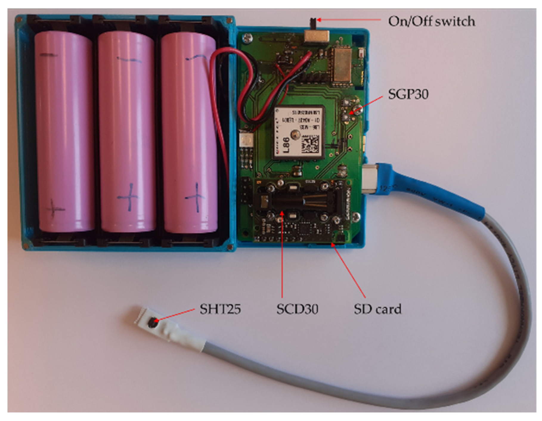
2.1. Sensor Device for IAQ Monitoring

The multi-sensor device was used for IAQ monitoring (see Figure 1). Its concept and prototype were developed at the Wroclaw University of Science and Technology, Poland. The equipment was designed to monitor several parameters of indoor air: temperature (T), relative humidity (RH), carbon dioxide (CO₂) concentration, and total volatile organic compound (TVOC) content. The device was fitted with low-cost sensors. Their detailed measurement characteristics are provided in

Table 1. Measurement characteristics of sensors applied in the multi-sensor device [34].

Sensor	Measured Parameter	Detection Principle	Measurement Range	Accuracy	Resolution	Repeatability	Long-Term Drift
SHT 25	T	Bandgap temperature sensor	−40 to 125 °C	Typ. ±0.2 °C	0.04 °C	±0.1 °C	<0.02 °C/yr
	RH	Capacity-type humidity sensor	0 to 95% RH	±1.8%RH	0.04%RH	±0.1%RH	<0.25%RH/yr
SCD30	CO2	Non-dispersive infrared (NDIR)	0–5000 ppm	±(30 ppm + 3% meas. Value)	-	±10 ppm	±50 ppm
SGP30	TVOCs and CO2eq	Metal oxide gas sensor (chemical resistor)	0.3–30 ppm ethanol 0–1000 ppm ethanol	Typ. 15% of meas. value	Typ. 0.2% of meas. value	-	Typ. 1.3% of meas. value
SGPC3	TVOCs	Metal oxide gas sensor (chemical resistor)	0.3–30 ppm ethanol 0–1000 ppm ethanol	Typ. 15% of meas. value	Typ. 0.2% of meas. value	-	Typ. 1.3% of meas. value

. Two sensors (SGP30 and SGPC3) were chosen to provide extensive information about VOCs in indoor air as they display different partial selectivity. Passive sensors’ exposure to the test gas was realized in the device (no induced gas flow). The measurements were performed continuously, with a temporal resolution of 2 s. The data records were logged into a file, which contained the time series of all measured parameters stamped with the time index. The data files were stored on the SD card inside the device prepared for download. The GPS unit was installed inside the sensor device to know its location. The device is small in size (12 × 8 × 2.5 cm) and has a small weight. It operates automatically and does not require the user’s attention. Batteries need to be replaced every five to seven days. Two devices of this kind involved in the IAQ monitoring study were taken into consideration for IAQ prediction in apartments using machine learning techniques and sensor data.

2.2. Apartments

Five apartments were included in this study. They were located in Wrocław (Poland). To obtain a diverse sample, we chose apartments that had different surroundings and standards and were used differently. The flats were distributed over various residential areas and located in buildings of different types and ages. The apartments’ size (from spacious apartments to studios), space arrangement (open kitchen and closed kitchen), as well as furnishing (from new and very modern to old and used) and appliances (type of ventilation, cooker, etc.), were different. Each apartment was occupied by one family, i.e., a couple or a couple with one child, which is typical in the city. However, we chose families with different cultural backgrounds, which implied specific lifestyles as well as individual dietary and cooking habits. More details regarding the characteristics of the individual apartments are presented in

Table 2. Detailed information about the apartments included in the IAQ monitoring study.

Feature	Apartment 1	Apartment 2	Apartment 3	Apartment 4	Apartment 5
Flat size	56 m2	35 m2	64 m2	27 m2	22.75 m2
Type of the kitchen	Open kitchen	Open kitchen	Closed kitchen	Open kitchen	Closed kitchen
Kitchen size	7 m × 5.5 m	3.5 m × 2 m	3 m × 2 m	4 m × 4 m	1.5 m × 3 m
Living room size		3.5 m × 3 m	2 m × 2.5 m		2.5 m × 3.5 m
Floor cover	Kitchen: panels Living room: panels and no carpet	Kitchen: tiles Living room: wood and no carpet	Kitchen: tiles Living room: panels with baby mattress	Kitchen: tiles Living room: tiles and woolen carpet	Kitchen: tiles Living room: panels and no carpet
Furniture	Not many items in the room. The furniture is new and made of fabric and wood.	Crowded with old furniture made of wood.	Crowded with old furniture made of wood and fiberboard.	Crowded with new furniture made of fabric and wood.	Crowded with old furniture made of wood and fabric.
Door between the kitchen and living room	None	None	Daytime: door opens while cooking. Nighttime: door mostly closed.	None	60% open 40% close
Kitchen window	None	None	None	Opens for 24 h	Opens for 24 h
Living room windows	Open for 24 h	Open for 24 h	Open from 6.00 a.m. to 7.00 p.m.	Open from 7.00 a.m. to 8.00 p.m.	Open for 24 h
Kitchen exhaust	No exhaust	Passive exhaust	Mechanical exhaust	Hood.	Hood and passive exhaust
Cooker	Induction	Gas	Gas	Induction	Gas
Cooking intensity	Twice a day (around 11.00 and 20.00)	Twice a day (around 8.00 and 18.00)	2–3 times a day (around 5.00, 12.00, 18.00)	1–2 times a day (around 9.00 and 14.00)	Twice a day (around 11.00 and 18.00)
Dishwashing	Dishwasher	Manually	Manually	Dishwasher	Manually
Location	Residential area	In the garden	In the green area (tress)	Residential area	By the main street
Type of building/age	Apartment building/new	Block of flats/old	Block of flats/old	Apartment building/new	Block of flats/old
Floor	5th	1st	1st	1st	5th
Occupants	2 adults	2 adults	2 adults with a baby	2 adults	2 adults
Additional information	One occupant fully works from home.	Occupants work from home 3 days a week. Smoker in the flat.	One occupant works from home 2 days a week.	Occupants fully work from home.	One occupant fully works from home.

. The inhabitants were asked to live their lives as usual to obtain representative results from the IAQ monitoring study.

2.3. IAQ Monitoring Study

The IAQ monitoring session in an individual apartment consisted of measuring indoor air parameters in the kitchen and the living room in parallel. The measurement point located in the kitchen (kitchen zone) was meant to provide the measurement data representing the overall kitchen atmosphere. Therefore, it was situated in the area designated for food preparation and consumption but at a distance from the cooker, spice storage area, and window/vent. The measurement point located in the living room (living room zone) was meant to provide the measurement data representing the actual living room atmosphere that people are exposed to. Therefore, it was situated centrally at the height of the breathing zone of a sitting person. One multi-sensor device was operated at each measurement point. One exemplar of the sensor device was used in the kitchen of all the flats included in this study, and another exemplar was used in the living room of all the apartments. Five apartments were examined in sequence. The monitoring session in a single apartment lasted at least seven days.

3. Methods

This work was dedicated to IAQ determination in apartments. We focused on IAQ prediction in the living room using the MLT model, which is supplied with the indoor air monitoring data collected by the dedicated sensor device located in the kitchen.

3.1. Prediction Model Structure

We chose to apply the multiple input–multiple output approach. The MLT model inputs were the results of IAQ monitoring in the kitchen, and the model predicted the air parameters in the living room. A diagram of the model structure is shown in Figure 2.

The following parameters were involved in model building: T, RH, CO₂ concentration, and the response of SGP30 and SGPC3 sensors. The MLT model was presented with the measurement data collected in the kitchen 1 min ahead of the prediction, and the model predicted the IAQ parameters in the living room 2 s later. The model had 5 × 29 inputs (5 indoor air parameters × 29 values of each parameter in the kitchen) and five outputs (5 indoor air parameters in the living room).

3.2. Prediction Models–MLT Models and Naive Approach

Five MLTs were applied: decision tree (DT), random forest regression (RFR), k-nearest neighbors (KNN) method, multilayer perceptron (MLP), and multiple linear regression (MLR). Additionally, the naive approach was chosen as a benchmark representing a minimum performance level attainable without any modeling effort.

3.2.1. Decision Tree (DT)

DT was originally designed for categorical data, but it may be also applied to continuous data, such as in this study. DT is constructed through recursive partitioning, where nodes are split based on input feature values to minimize the overall variance or another specified metric considering all output variables. The recursive process continues until a stopping criterion is met, such as a specified tree depth or a minimum number of samples in a leaf node [35]. Each leaf contains a constant value, usually an average value of the target attribute, replaced in the model tree by a linear or nonlinear regression function. When making predictions for a new data point, the tree is traversed from the root to a leaf, and the predicted values for all the output variables are derived from the values associated with that leaf [36]. Building a predictive model using DT has two goals: to accurately predict the response variable from the input data vector and to uncover the structural relationships between the response and measured variables. These dual objectives emphasize the role of the model in precise forecasting and uncovering underlying dependencies in the observed data [37].

3.2.2. Random Forest Regression (RFR)

Random forest includes multiple decision trees. It provides a robust and stable estimate that handles complex relationships and leverages predictive performance [38]. RFR applies bootstrap sampling to create multiple subsets of the original dataset by randomly sampling with replacement [39]. The subsets serve as the training data for an individual decision tree, introducing diversity to minimize overfitting [40]. In this work, RFR was composed of 100 decision trees. This number was chosen arbitrarily to account for the description of a complex relationship between independent and dependent variables. Each decision tree independently predicts five outputs based on the provided 5 × 29 input features. Subsequently, the algorithm aggregates the results from all individual trees and calculates their meaning as the final result [41].

3.2.3. K-Nearest Neighbors (KNN)

KNN is a non-parametric approach that extracts patterns and relationships between independent and dependent variables [42,43]. The algorithm proceeds by applying a distance metric to identify the k-nearest neighbors from the training dataset based on the input feature similarity [44]. In this work, the number of neighbors was set to k = 5 based on preliminary simulations. Euclidean distance was employed as a distance metric. Subsequently, the weights of the k neighbors were calculated for each output based on their proximity to the new data point. The distance-weighting scheme was applied where closer neighbors had a higher influence. The numerical value for the new data point was predicted by calculating the weighted average of the target values of the KNN using Equation (1) [45].

$${\widehat{y}}_j=\sum _{i=1}^K\frac{w_i}{\sum _{i=1}^K{w}_i}·y_{i,j}$$

(1)

where ${\widehat{y}}_j$ is the predicted value of the j-th output variable, $y_{i,j}$ is the target value of the j-th output variable for the i-th neighbor, and $w_i$ denotes the weight assigned to the i-th neighbor based on its proximity to the new data point.

3.2.4. Multilayer Perceptron (MLP)

MLP is a feedforward artificial neural network, consisting of neurons fully connected through adaptable synaptic weight [31]. In this study, the MLP model consisted of an input layer, an output layer, and two hidden layers comprising 100 nodes each. MLP training involved pairing input and target values. During forward propagation, input features traverse the network, generating predictions at the output layer. The disparity between observed and predicted values is calculated and this information is then propagated backwards [32]. The Adam optimizer was employed to adjust the weights between neurons. The iterative process was repeated for a maximum of 500 iterations until the model converged. We compared MLPs fitted with linear (in MLP1) and nonlinear (in MLP2) activation functions. The nonlinear transfer function was Rectifier Linear Unit (f(x) = max(0,x)) from Scikit Learn. The linear transfer function was Identity (f(x) = x) from Scikit Learn.

3.2.5. Multiple Linear Regression (MLR)

MLR is an extension of the basic linear regression method to handle multiple independent variables and multiple target parameters simultaneously, expressed as Equation (2).

$$y_i=a_{0i}+a_{1i}{x}_{1i}+a_{2i}{x}_{2i}+\cdots +a_{ni}{x}_{ni}+{\epsilon }_i$$

(2)

where $y_i$ is the ith dependent variable, $x_{1i},x_{2i},\dots ,x_{ni}$ are independent predictors $a_{1i},a_{2i},\dots ,a_{ni}$ are regression coefficients of each predictor, including $a_{0i}$—the ith intercept, and ${\epsilon }_i$ is the i-th residual [46,47]. The regression coefficients indicate the alteration of the dependent variables caused by a unit increase in the predictor variables. These coefficients facilitate a comparative assessment of the relative significance of each predictor for model output, providing insights into their respective impacts within the regression model [47]. The residuals indicate the spread of the true values of the target parameter around the regression line [46].

3.2.6. Naive Approach

The naive approach assumes that the predicted value is the same as the value of the predictor one timestep ahead of prediction. In this work, the naive approach was realized by assuming that the air parameters in the living room have the same values as those most recently observed in the kitchen. Basically, upon the availability of IAQ monitoring in the kitchen, no additional data manipulation was needed to determine the conditions in the living room if the naive approach turned out best.

The naive approach was proposed as a reference for judging the objective value of MLTs’ prediction. It allowed us to reach out beyond just ranking the MLTs’ performance and determine whether the MLTs’ performance was truly good or not. The performance of the naive approach showed what could be attained without any computational effort involving a model that represents a generic relationship between the kitchen’s and living room’s IAQ.

3.3. Prediction Model Validation

A rigid and comprehensive cross-validation procedure was applied to achieve an exhaustive performance evaluation of all MLTs included in our analysis. The schema explaining this procedure is shown in Figure 3.

The cross-validation procedure consisted of five folds. In a single fold, the data from four apartments were used for model training, and the data from one remaining apartment were applied for model testing. In each fold, the data used for testing were associated with a different apartment.

By applying the presented cross-validation approach, we asked about the common character of the relationship between the IAQ in the kitchen and in the living room in various apartments. If confirmed, the MLT models could be claimed as having high generalization potential and being applicable in different apartments than those providing data for model training.

3.4. Performance Metrics

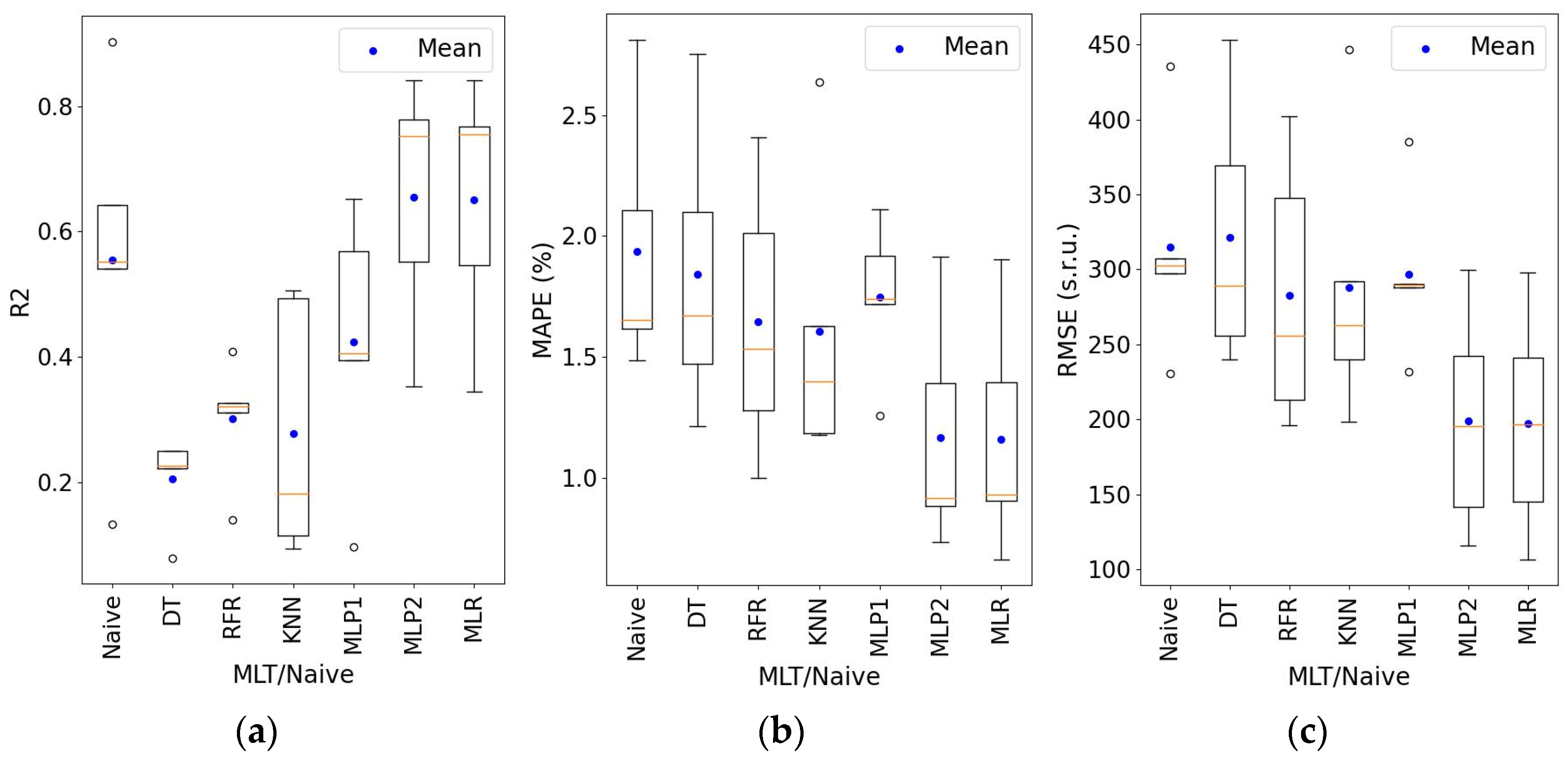
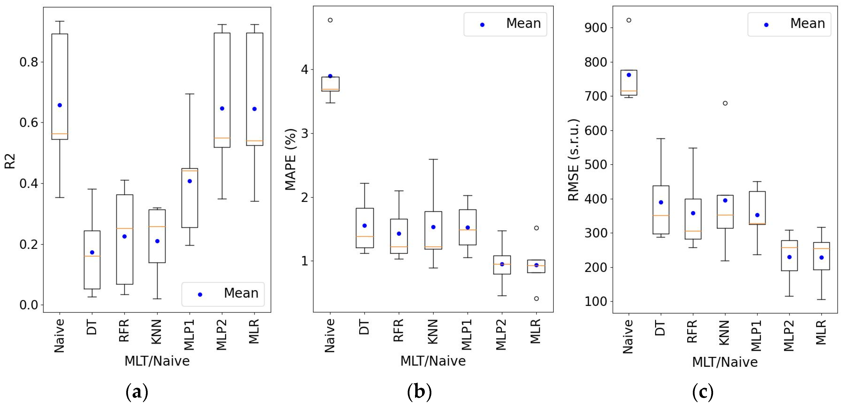
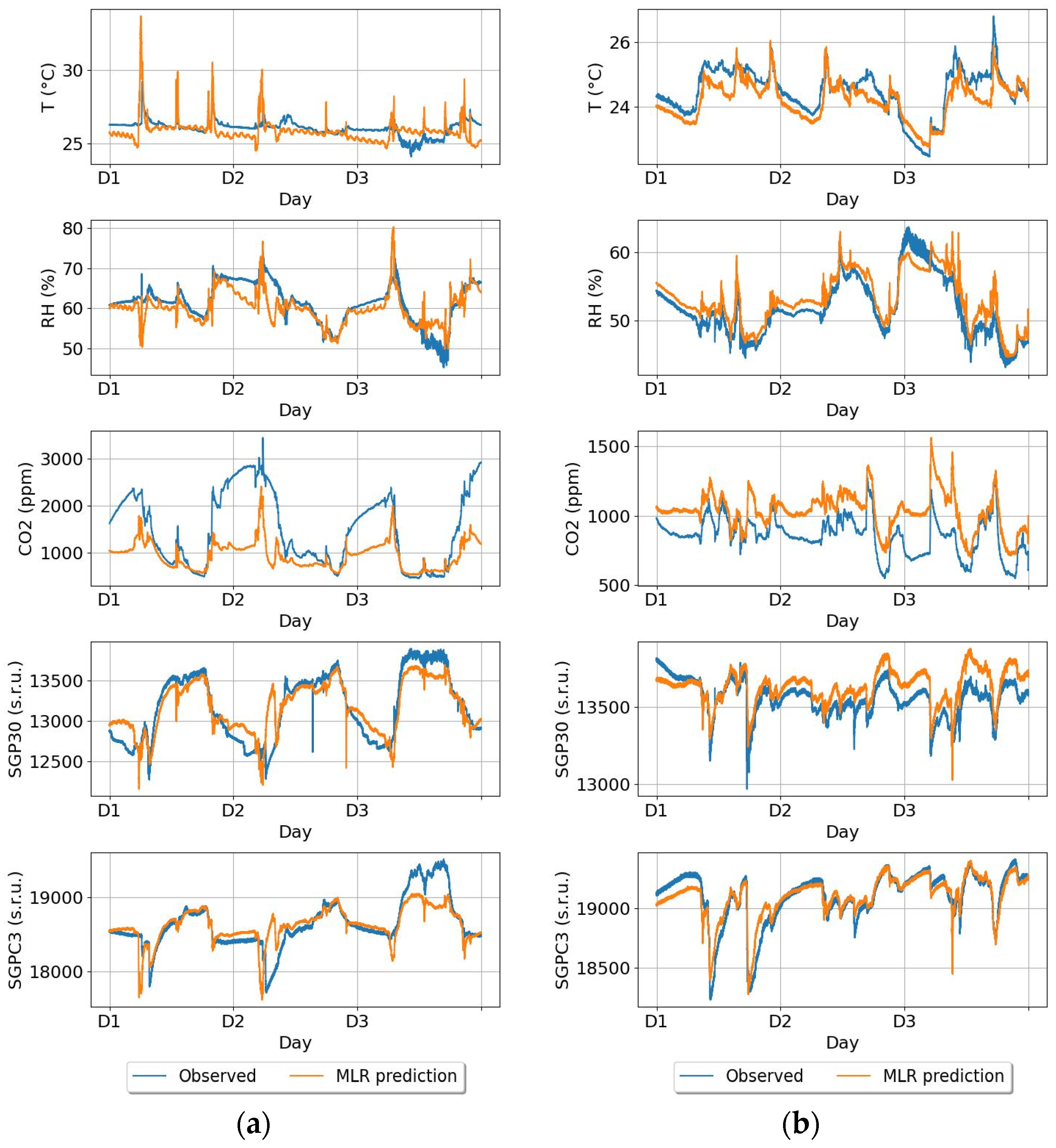
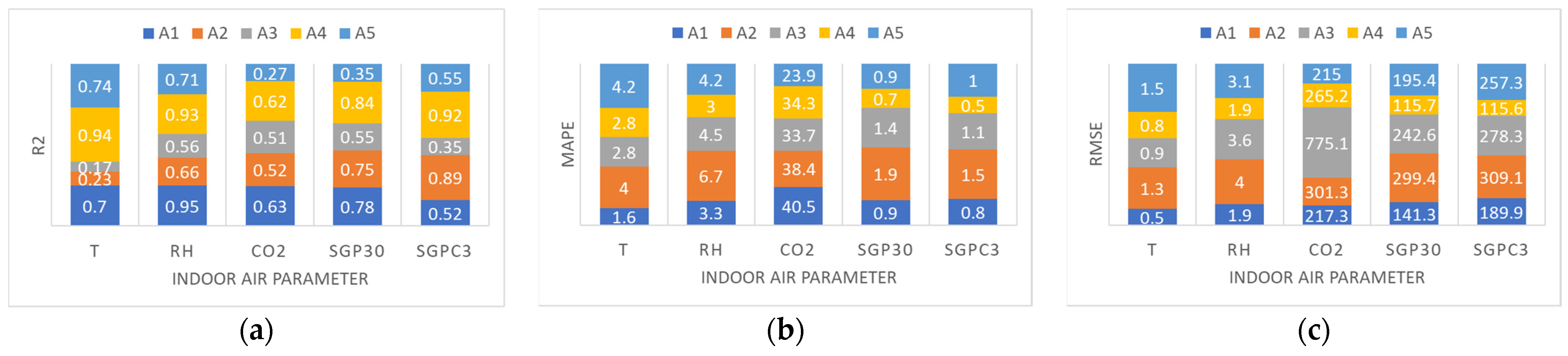
The performance of MLT models was evaluated using a coefficient of determination (R²) and two prediction errors: root mean squared error (RMSE) and mean absolute percentage error (MAPE).

R² is a measure applied to characterize the quality of the predictive model. It reflects the effectiveness of the regression model in fitting the data. The coefficient of determination, R², was calculated using Equation (3) [48].

$$R^2=\frac{\sum _{i=1}^N{(p_i-\overline{r})}^2}{\sum _{i=1}^N{(r_i-\overline{r})}^2}$$

(3)

where $r_i$ is the observed data, $p_i$ is the predicted data, $\overline{r}$ is the observed data average, and N is the size of the dataset. $R^2$ represents the fraction of target variable variability that has been explained by the model [49]. The range is $R^2\in 〈0,1〉$, and values close to one indicate a high-quality model.

Errors were used to characterize the quality of prediction, and their low values indicated high-quality prediction.

RMSE calculates the average squared difference between the observed and predicted data, as given by Equation (4).

$$RMSE=\sqrt{\frac{1}{N}\sum _{i=1}^N{(p_i-r_i)}^2}$$

(4)

where $r_i$ is the observed data, $p_i$ is the predicted data, and N is the size of the dataset.

RMSE is expressed in the same units as the predicted variable; so, its magnitude is easy to interpret as low or high for a particular physical quantity. On the other hand, RMSE use is limited when it comes to comparing the error of determining distinct quantities. This error measure is sensitive to outliers due to the squaring mechanism [49].

MAPE calculates the absolute difference between the observed and predicted data and views it as a fraction of the observed data, as given by Equation (5) [48].

$$MAPE=\frac{1}{N}\sum _{i=1}^N\frac{\left|p_i-r_i\right|}{r_i}·100\%$$

(5)

where $r_i$ is the observed data, $p_i$ is the predicted data, and N is the size of the dataset. MAPE represents the percentage error, providing an understanding of how off the predictions are in relative terms. In this work, it was chosen as the performance metric to overcome the limitation of RMSE in comparing predictions of different air parameters.

4. Results

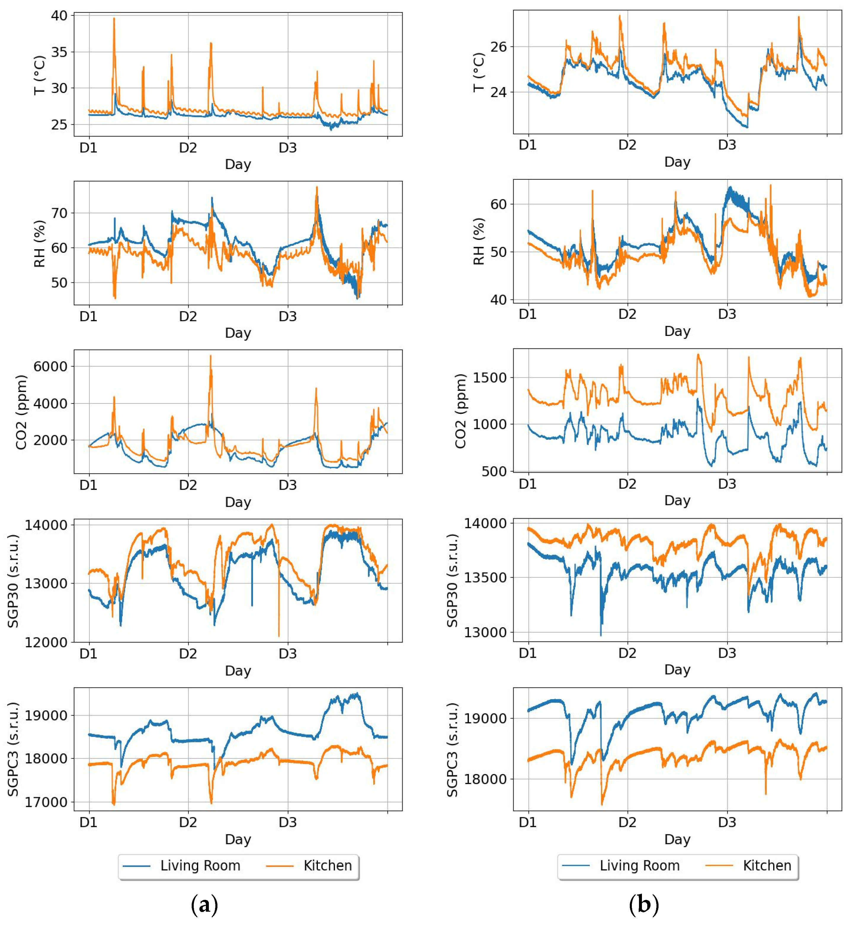
4.1. Selected Results of IAQ Monitoring in Apartments

Figure 4 shows the data collected during the IAQ monitoring study. It includes the results of three days of measurements performed in two apartments (apartments A3 and A4). The indoor air parameters, i.e., T, RH, CO₂ concentration, SGP30 sensor response (indicative for TVOC content), and SGPC3 sensor response (also indicative for TVOC content) are displayed as the time series collected at the measurement point located in the kitchen and the living room.

The visual inspection of Figure 3 allows for several important observations. 1. Different air parameters monitored in one apartment, even at the same measurement point, displayed distinct temporal variation patterns. This fact justifies predicting each of these parameters individually. 2. The time series of a particular air parameter measured in the kitchen and in the living room in the same apartment behaved similarly in time. It supports the idea of using IAQ monitoring in one of these locations, e.g., in the kitchen, to determine the IAQ in another location, e.g., in the living room. 3. It should be emphasized that the similarity between the temporal variation of a particular air parameter measured in the kitchen and the living room in the same apartment was observed in all the flats. This fact encourages the examination of the relationship between IAQ in the two locations for various flats. If confirmed, one MLT model could be developed to predict IAQ in multiple flats. 4. The temporal variation patterns of one air parameter in two apartments are distinct. This could raise some concerns about the possibility of MLT prediction model transfer between apartments.

It shall be noted that the difference between the values of individual air parameters in the kitchen and the living room is partially due to the offset of sensor devices. In real conditions, frequent calibration is difficult to realize. In this work, we addressed the problem in two ways. First, a check was made to confirm that the responses of all devices to the individual air parameters were highly correlated and to identify potential shifts between them. For that purpose, before deployment in the flats, all the devices were left in one room for 3 × 24 h to perform comparative measurements. This approach surely has its limitations, but it may be easily and widely applied in practice. Second, in this study, the offset did not have any impact on the results of the MLT performance assessment. This problem was overcome by using the same exemplar of a sensor device for measurements in all kitchens and another exemplar for measurements in all living rooms.

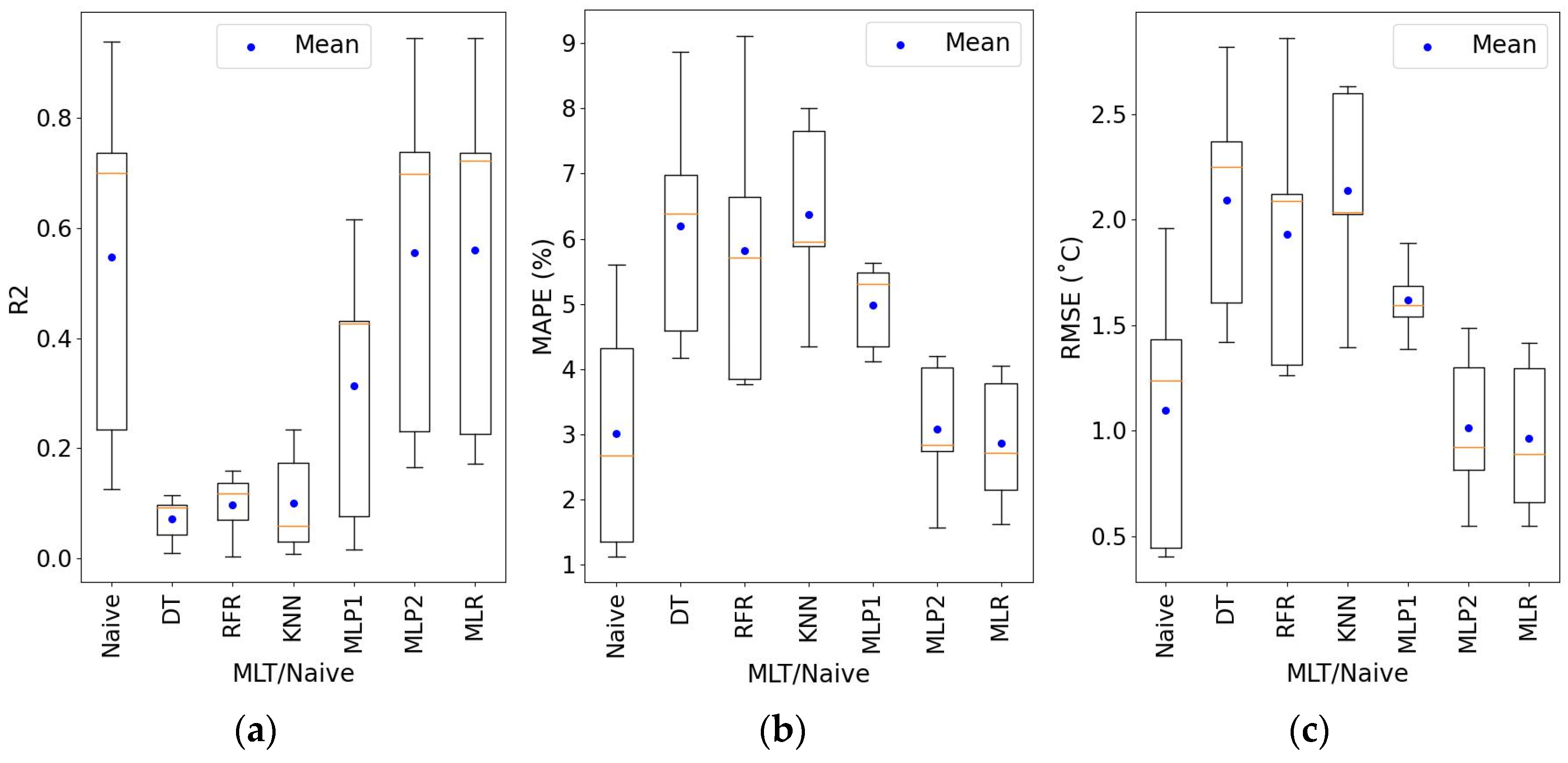
4.2. Temperature Prediction

Figure 5 compares the performance of MLTs in living room temperature prediction based on IAQ monitoring in the kitchen. The following performance metrics were used: R² (Figure 5a), MAPE (Figure 5b), and RMSE (Figure 5c). Their median values are shown in

Table 3. Summary of median performance metrics: R², MAPE, and RMSE for all MLTs and the naive approach. The performance metrics where MLT outperformed the benchmark are highlighted.

MLT/ Naive	R2					RMSE					MAPE [%]
	T	RH	CO2	SGP30	SGPC3	T [°C]	RH [%]	CO2 [ppm]	SGP30 [s.r.u.]	SGPC3 [s.r.u.]	T	RH	CO2	SGP30	SGPC3
DT	0.09	0.31	0.10	0.23	0.16	2.3	6.3	335	289	351	6.4	8.0	33.7	1.7	1.4
RFR	0.12	0.40	0.16	0.32	0.25	2.1	5.3	278	256	306	5.7	6.9	30.2	1.5	1.2
KNN	0.06	0.40	0.08	0.18	0.26	2.0	5.2	252	263	353	6.0	7.4	29.2	1.4	1.2
MLP1	0.43	0.58	0.05	0.41	0.44	1.6	4.6	360	290	328	5.3	7.2	39.7	1.7	1.5
MLP2	0.7	0.71	0.52	0.75	0.55	0.9	3.1	265	195	257	2.8	4.2	34.3	0.9	1.0
LR	0.72	0.71	0.51	0.75	0.54	0.9	3.3	277	197	255	2.7	4.4	36.4	0.9	0.9
Naive	0.7	0.72	0.38	0.55	0.56	1.2	4.1	491	303	715	2.7	6.6	66.1	1.7	3.7

.

As shown in Figure 5a, linear MLTs offered the best quality in temperature prediction. Coefficients of determination were highest in the case of MLR (R² = 0.72) and MLP2 (R² = 0.70). The naive approach (R² = 0.70) offered comparable quality, while the quality of nonlinear MLTs (DT, RFR, KNN, and MLP1) was very low, as shown by a small R² (0.09–0.43). Considering the percentage error of T prediction, the naive approach yielded the lowest score of MAPE (2.68%) (Figure 5b). Still, it was comparable to the error offered by linear methods MLR (MAPE = 2.71%) and MLP2 (MAPE = 2.84%). When applying nonlinear MLTs, the prediction errors were considerably higher (MAPE = 5.30–6.38%). Regarding the RMSE of T prediction (Figure 5c), the errors were smallest in the case of MLR (RMSE = 0.89 °C) and MLP2 (RMSE = 0.92 °C), which are linear MLTs. They outperformed the naive approach, with RMSE = 1.24 °C. When using nonlinear MLTs, temperature prediction was loaded with bigger errors (RMSE = 2.04–2.25 °C). In summary, it is possible to predict the temperature in the living room of the apartment based on IAQ monitoring in the kitchen with an error smaller than 1 °C using linear MLTs. It is crucial to note that this result was achieved by prediction models trained on IAQ monitoring data collected in different apartments than where the prediction was realized. The best prediction was achieved using MLR, and the quality of this model was the highest. Such a result could not be attained with the naive approach. Nonlinear MLTs were an even less viable alternative to linear methods in the case of temperature predictions.

4.3. Relative Humidity Prediction

Figure 6 compares the performance of MLTs in living room relative humidity prediction based on IAQ monitoring in the kitchen. The following performance metrics were used: R² (Figure 6a), MAPE (Figure 6b), and RMSE (Figure 6c). Their median values are shown in Table 3.

As shown in Figure 6a, linear MLTs offered the best quality in relative humidity prediction. Coefficients of determination were highest in the case of MLR (R² = 0.72) and MLP2 (R² = 0.71), while the naive approach (R² = 0.719) offered a comparable performance. The quality of nonlinear MLTs (DT, RFR, KNN, and MLP1) was very low, as shown by a small R² (0.31–0.57). Based on Figure 6b, linear methods MLR (MAPE = 4.42%) and MLP2 (MAPE = 4.18%) yielded the lowest percentage error of RH prediction. In the case of the naive approach, the error was higher (MAPE = 6.60%), and it still increased when applying nonlinear MLTs (MAPE = 6.86–8.01%RH). Regarding the RMSE of RH prediction (Figure 6c), linear methods MLR and MLP2 offered the lowest errors of RMSE (RMSE = 3.27%RH and RMSE = 3.07%RH, respectively). They outperformed the naive approach (RMSE = 4.14%RH) and nonlinear MLTs as with these models, RH prediction was still greater (RMSE = 4.64–6.26%RH). In conclusion, it is possible to predict relative humidity in the living room based on IAQ monitoring in the kitchen with an error smaller than 3.50%RH using linear models. Similar to T, it is crucial to note that this result was achieved by prediction models trained on IAQ monitoring data collected in different apartments and not where the prediction was realized. The best prediction was achieved using MLR, and the quality of this model was the highest. Such a result could not be attained by the naive approach. Nonlinear MLTs were even less effective for RH prediction.

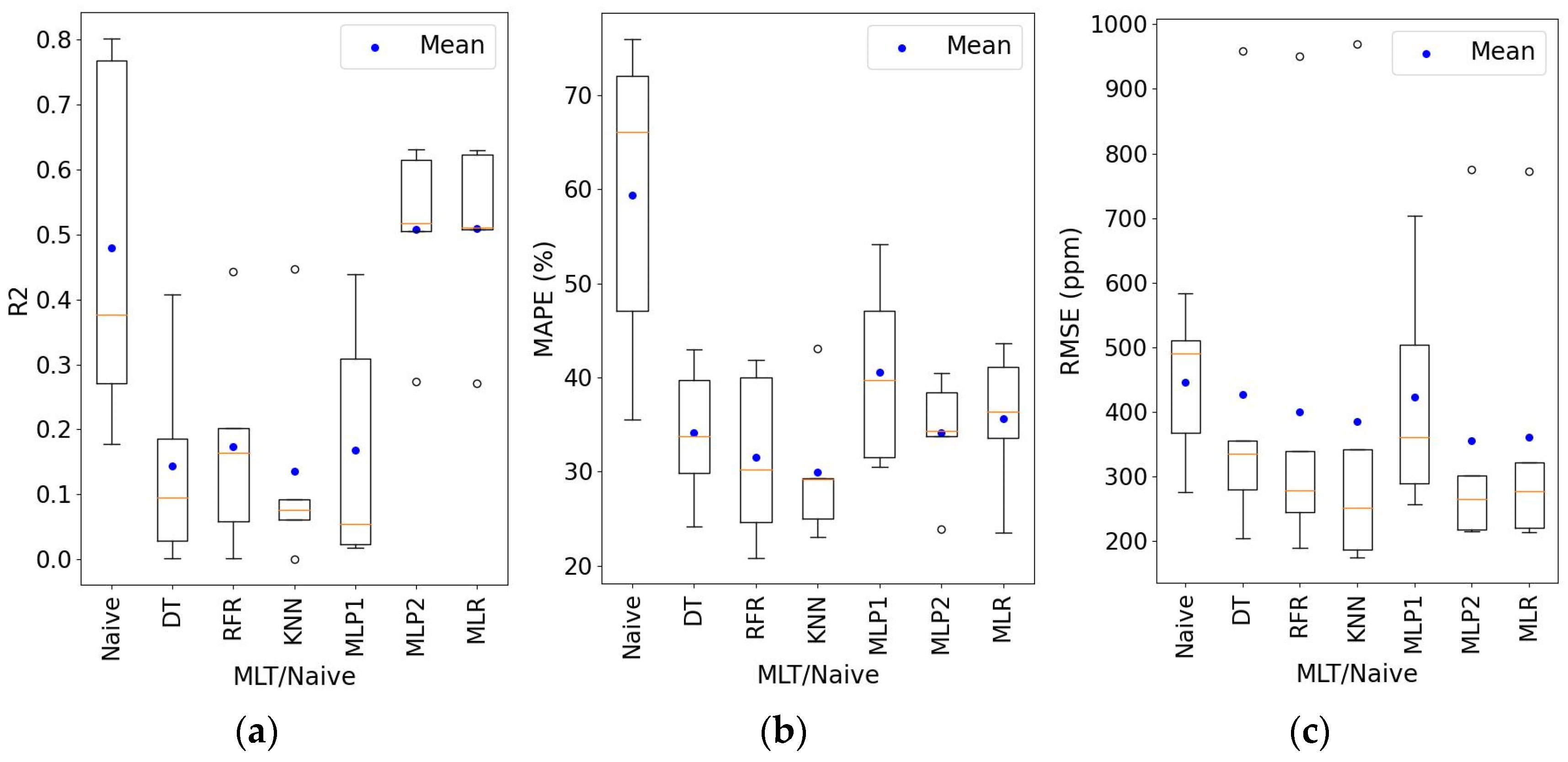
4.4. CO₂ Concentration Prediction

Figure 7 compares the performance of MLTs in predicting CO₂ concentration in the living room based on IAQ monitoring in the kitchen. The following performance metrics were used: R² (Figure 7a), MAPE (Figure 7b), and RMSE (Figure 7c). Their median values are shown in Table 3.

As can be seen in Figure 7a, among MLTs used to predict CO₂ concentration, linear methods MLR and MLP2 showed the highest coefficients of determination (R² = 0.51 and R² = 0.52, respectively). Yet, these values were low in a general sense, and they indicated the poor quality of prediction models. In the case of the naive approach, R² = 0.38 was still smaller. Coefficients of determination for nonlinear MLTs (R² = 0.05–0.16) were so small that they precluded the use of these models for predicting CO₂ concentration. Interestingly, as indicated in Figure 7b, the relative errors of CO₂ concentration prediction using linear methods (MAPE = 34.34–36.40%) were similar to those for nonlinear methods (MAPE = 29.11–39.69%). In addition, MLTs outperformed the naive approach (MAPE = 66.1%). Similar to the case of MAPE, the RMSE of CO₂ concentration prediction using linear methods (RMSE = 265–277 ppm) was similar to that obtained using nonlinear methods (RMSE = 252 ppm–360 ppm), and all of them were smaller than the error offered by the naive approach, with RMSE = 491 ppm (see Figure 7c). In summary, it should be underlined that MAPE errors of tens of percentages, as well as RMSE errors of several hundred ppm, are large and not attractive results. Thus, based on the performed analysis, the prediction of CO₂ concentration in the living room, based on IAQ monitoring in the kitchen, was ineffective while using MLTs trained on the data collected in different apartments.

4.5. TVOC Content Prediction (SGP30 Sensor Response)

Figure 8 compares the performance of MLTs in predicting TVOC content (evaluated using an SGP30 sensor) in the living room based on IAQ monitoring in the kitchen. The following performance metrics were used: R² (Figure 8a), MAPE (Figure 8b), and RMSE (Figure 8c). Their median values are shown in Table 3.

As shown in Figure 8a, linear MLTs offered the best quality in predicting TVOC content, evaluated using the SGP30 sensor. Coefficients of determination were highest in the case of MLR (R² = 0.75) and MLP2 (R² = 0.75). The naive approach (R² = 0.55) showed lower performance. The quality of nonlinear MLTs (DT, RFR, KNN, and MLP1) was very low, as shown by small R² (0.18–0.41). Based on Figure 8b, linear methods MLR (MAPE = 0.93%) and MLP2 (MAPE = 0.91%) yielded the lowest percentage error of TVOC content prediction. In the case of the naive approach, the error was higher (MAPE = 1.65%). The lowest MAPE achievable using a nonlinear technique was offered by RFR (MAPE =1.53%). Regarding the RMSE of TVOC content prediction (Figure 8c), all the MLTs (RMSE = 195–289 s.r.u.) offered lower errors than the naive approach (RMSE = 302 s.r.u). In addition, the errors attained using linear MLTs were the smallest (RMSE = 195–197 s.r.u). In conclusion, it is possible to predict TVOC content, evaluated using an SGP30 sensor, in the living room based on IAQ monitoring in the kitchen with a percentage error of less than 1%, which corresponds to about 196 s.r.u. using linear models. Similar to T and RH, it is crucial to note that this result was achieved by prediction models trained on IAQ monitoring data collected in different apartments and not where the prediction was realized. The best prediction was achieved using MLR, and the quality of this model was the highest. Non-linear models, despite their poor quality, outperformed the naive approach in terms of prediction error.

4.6. TVOC Content Prediction (SGPC3 Sensor Response)

Figure 9 compares the performance of MLTs in predicting TVOC content (evaluated using SGPC3 sensor) in the living room based on IAQ monitoring in the kitchen. The following performance metrics were used: R² (Figure 9a), MAPE (Figure 9b), and RMSE (Figure 9c). Their median values are shown in Table 3.

As shown in Figure 9a, all MLTs applied to predict TVOC content, evaluated using the SGPC3 sensor, demonstrated lower quality (R² = 0.16–0.54) than the naive approach (R² = 0.56). These values indicated the modest quality of models in general. Still, linear models MLR and MPL2 were featured by the highest R², with R² = 0.54 and R² = 0.55, respectively. The quality of nonlinear MLTs was very small (R² = 0.16–0.44). Based on Figure 9b, all the MLTs offered lower errors (MAPE = 0.93–1.49%) than the naive approach (MAPE = 3.70%). In the case of linear MLTs, i.e., MLR and MPL2, the errors were smallest, with MAPE = 0.93% and MAPE = 0.95%, respectively. Also, regarding the RMSE, all the MLTs (RMSE = 255–353 s.r.u.) offered lower errors compared to the naive approach (RMSE (naive) = 715 s.r.u.) (see Figure 9c). The errors attained using linear MLTs, i.e., MLR and MPL2, were the smallest (RMSE = 255 s.r.u. and RMSE = 257 s.r.u., respectively). In conclusion, it is possible to predict TVOC content, evaluated using an SGPC3 sensor, in the living room based on IAQ monitoring in the kitchen, using linear models, with a percentage error of less than 1%. Similar to T, RH, and TVOC content based on the SGP30 sensor it is crucial to note that this result was achieved by prediction models trained on IAQ monitoring data collected in different apartments and not where the prediction was realized. The best prediction was achieved using MLR, which was also one of the highest-quality models. Although the quality of the naive approach was the highest, it was outperformed by all the MLTs in terms of prediction errors.

5. Discussion

The summary of median performance metrics (R², MAPE, and RMSE) for all MLTs, together with the naive approach, is presented in Table 3. Figure 10 shows the performance metrics of one of the best MLT, i.e., multiple linear regression (MLR), for tests on the data from the individual apartments, i.e., A1, A2, A3, A4, and A5. The comparison of the observed time series of indoor air parameters and the time series predicted by the MLR model is displayed in Figure 11. Apartments A3 and A4 were chosen for presentation, as they were also referred in Figure 4.

Based on the results of this study, several observations could be made. (1) In the apartments, there exists a co-dependency between indoor air parameters in the kitchen and the living room. (2) This relationship has a common component that is pertinent in multiple apartments despite their versatility. (3) The relationship may be exploited by MLTs and utilized for prediction purposes. (4) Various MLTs perform differently in predicting living room IAQ based on kitchen air monitoring. (5) The prediction of distinct indoor air parameters is not equally effective. (6) MLT model performance varies among flats.

R² characterizes the percentages of variance of the individual air parameters in the living room explained by prediction models. Based on the R² medians shown in Table 3, the highest percentages of variance explained for the individual air parameters in the living room were R² = 0.72 (MLR for T), R² = 0.72 (naive for RH), R² = 0.52 (MLP2 for CO₂), R² = 0.75 (MLR and MLP2 for TVOC based on SGP30 sensor), and R² = 0.56 (naive for TVOC based on SGP30 sensor). Given these results, the existence of co-dependency between indoor air parameters in the kitchen and the living room of apartments could be confirmed. Due to the applied cross-validation procedure (see Section 3.3), the calculated coefficients of determination reflect the magnitude of the component of the relationship, which is common in multiple apartments despite their versatility.

Despite the problem’s complexity, high-performance models could be attained upon a favorable selection of training and test apartments. The analysis of plots in Figure 5a to Figure 9 reveals a considerable spread of R² for a particular MLT applied to predict an individual air parameter in five folds. The spread comes from the fact that model performance was dependent on the combination of apartments providing training and test data in the individual folds. In particular, for some combinations of apartments, R² was objectively very high, as shown by its maximum values, which were R² = 0.94 (MLR and MLP2 for T), R² = 0.94 (MLR and MLP2 for RH), R² = 0.63 ( MLR and MLP2 for CO₂), R² = 0.84 (MLR and MLP2 for TVOC, based on the SGP30 sensor), and R² = 0.92 (MLR and MLP2 for TVOC, based on the SGP30 sensor). Additional work could be undertaken to identify the similarity criteria allowing for apartment grouping to support the selection of the representative training data and allowing for the preparation of MLT models applicable to certain categories of apartments. With this option, the necessity of apartment-specific model parametrization could be eliminated.

Based on our analysis, MLTs may be effectively applied to predict living room IAQ based on indoor air monitoring in the kitchen. Moreover, this work establishes that linear approaches yielded the best results, whereas nonlinear MLTs fell short in predicting indoor air parameters accurately. As already mentioned, a high R² was found for linear MLTs. In addition, they offered the smallest prediction errors in the case of all indoor air parameters, except for CO₂. The minimum percentage errors were MAPE = 1.57% (MLP2 for T), MAPE = 2.97% (MLP2 for RH), MAPE = 20.83% (RFR for CO₂), MAPE = 0.66% (MLR for TVOC based on the SGP30 sensor), and MAPE =0.41% (MLR for TVOC based on the SGP30 sensor). The minimum RMSEs of prediction were RMSE = 0.5 °C (MLR for T), RMSE = 1.8%RH (MLR for RH), RMSE = 174 ppm (KNN for CO₂), RMSE = 106 s.r.u. (MLR for TVOC based on the SGP30 sensor), and RMSE = 106 s.r.u. (MLR for TVOC, based on the SGP30 sensor). Based on the fact that the best-quality models were linear ones (highest R²) and that they also offered the best prediction (lowest MAPE and RMSE), it could be claimed that the relationship between indoor air parameters in the living room and kitchen in the apartment is linear. This conclusion refers to a short-term perspective as the prediction was based on the data collected one minute before the prediction.

Table 3 indicates the MLTs’ performance regarding the naive approach by highlighting the performance metrics where MLTs outperformed the benchmark. As shown, in terms of median performance metrics, linear MLTs (MLR and MLP2) allowed us to build higher-quality models for all indoor air parameters except for CO₂ and TVOC based on the SGP30 sensor. The prediction errors made by linear MLTs were all lower than achievable using the naive approach. Additionally, as shown in Figure 10, linear models adequately captured and reproduced the temporal variability of indoor air parameters in the living room. The observed and predicted time series well matched each other in terms of timing of sudden increase or decrease as well as the magnitude of parameters change. These results justify applying linear MLTs for IAQ prediction in the considered framework by providing an added value compared to the naive approach. The fact that the results of the naive approach are very close to the results of the best MLTs suggests that the most recent results of measurements contribute greatly to an effective prediction. Still, the fact that the MLTs performed better than the naive approach in the framework of cross-suggests that the domination would increase when a prediction model is developed for a particular category of apartments, and even more so if the model was prepared for an individual apartment.

Considering that five apartments were included in this study, the MLTs had to cope with a considerable diversity of object characteristics. It was associated with kitchen type (open or closed), the apartment ventilation system, the occupants’ lifestyle and cooking habits, occupancy patterns, surroundings, etc. These multiple factors resulted in the diverse indoor conditions in the individual apartments. The results of their monitoring provided complex input data for MLT models, which ultimately influenced their performance. As displayed in Figure 11b,c, the most accurate prediction was attained in the case of apartments A1 and A4. Excluding CO₂, average MAPE was MAPE = 1.70 ± 1.15% (for flats A1 and A4) and MAPE = 2.85 ± 1.85% (for flats A2, A3, and A5). Based on Figure 11a, the R² of MLR was also highest when models were tested on the data from these apartments. Excluding CO₂, average R² was R² = 0.75 ± 0.13 (for flats A1 and A4) and R² = 0.45 ± 0.21 (for flats A2, A3, and A5). Common features of apartments A1 and A4, which made them distinct from the others, were that they were located in new apartments, fitted with an open kitchen and induction cooker. Given the problem considered in this work, it is likely that the key factor is an open kitchen, offering good mixing between the air in the kitchen and living room zones. Hence, open-kitchen apartments could be the category of choice for the practical application of the approach presented in this paper.

6. Conclusions

The results of this study allow for several conclusions to be drawn.

In apartments, there exists a co-dependency between indoor air parameters in the kitchen and living room. The individual air parameters in the two locations display similar patterns of temporal variation.

The relationship may be exploited by MLTs and utilized for IAQ prediction in the living room. As multiple indoor air parameters shall be determined to attain a comprehensive representation of indoor conditions, the multiple input–multiple output approach is favored to limit the number of applied models.

For the cross-validation procedure, where training and test apartments are distinct, MLTs outperform the naive approach. Hence, the relationship between the living room and kitchen IAQ has a component that is common for multiple apartments despite their versatility and allows for prediction model transfer between apartments.

Better tuning of MLT models may be attained by applying apartment categorization. In particular, open-kitchen apartments could be the category of choice for the practical application of our approach as the most accurate prediction was demonstrated for such apartments.

Based on our study, linear MLTs, such as MLR and MLP with linear transfer functions, performed best. They were featured by the highest coefficients of determination, mostly exceeding an R² of 0.8, and they offered the lowest prediction errors compared to nonlinear models, such as DT, RFR, KNN, and MLP with nonlinear transfer functions.

The prediction of distinct indoor air parameters was not equally effective. Based on the lowest percentage error, reasonable predictions were attained for indoor air temperature (MAPE = 1.57%), relative humidity (MAPE = 2.97%RH), and TVOC content (MAPE = 0.41%), while CO₂ prediction was loaded with a high error (MAPE = 20.83%).

This work successfully exploits the relationship between IAQ in the kitchen and living room, encouraging future research endeavors aimed at refining predictive models and improving IAQ management strategies in apartments.

References

1. World Air Quality Report. 2020. Available online: https://www.jagranjosh.com/general-knowledge/world-air-quality-report-2020-all-about-delhi-being-the-most-polluted-capital-of-the-world-1615966983-1 (accessed on 12 May 2024).
2. United States Environmental Protection Agency. Introduction to Indoor Air Quality. 2023. Available online: https://www.epa.gov/indoor-air-quality-iaq/introduction-indoor-air-quality (accessed on 12 May 2024).
3. Shooshtari, M.; Salehi, A. An electronic nose based on carbon nanotube -titanium dioxide hybrid nanostructures for detection and discrimination of volatile organic compounds. Sens. Actuators B Chem. 2022, 357, 131418. [Google Scholar] [CrossRef]
4. Peters, T.; Zheng, C. Evaluating Indoor Air Quality Monitoring Devices for Healthy Homes, Buildings. Buildings 2024, 14, 102. [Google Scholar] [CrossRef]
5. Yasin, A.; Delaney, J.; Cheng, C.-T.; Pang, T.Y. The Design and Implementation of an IoT Sensor-Based Indoor Air Quality Monitoring System Using Off-the-Shelf Devices. Appl. Sci. 2022, 12, 9450. [Google Scholar] [CrossRef]
6. Tsoulou, I.; He, R.; Senick, J.; Mainelis, G.; Andrews, C.J. Monitoring summertime indoor overheating and pollutant risks and natural ventilation patterns of seniors in public housing. Indoor Built Environ. 2023, 32, 992–1019. [Google Scholar] [CrossRef]
7. Liu, J.; Dai, X.; Lia, X.; Jia, S.; Pei, J.; Sun, Y.; Lai, D.; Shen, X.; Sun, H.; Yin, H.; et al. Indoor air quality and occupants’ ventilation habits in China: Seasonal measurement and long-term monitoring. Build. Environ. 2018, 142, 119–129. [Google Scholar] [CrossRef]
8. Cheung, P.K.; Jim, C.Y. Indoor air quality in substandard housing in Hong Kong. Sustain. Cities Soc. 2019, 48, 101583. [Google Scholar] [CrossRef]
9. Kraus, M.; Senitková, I.J. Particulate Matter Mass Concentration in Residential Prefabricated Buildings Related to Temperature and Moisture, World Multidisciplinary Civil Engineering-Architecture-Urban Planning Symposium—WMCAUS. IOP Conf. Ser. Mater. Sci. Eng. 2017, 245, 042068. [Google Scholar] [CrossRef]
10. Tahmasebi, F.; Wang, Y.; Cooper, E.; Shimizuhttps, D.G.; Stamp, S.; Mumovic, D. Window operation behaviour and indoor air quality during lockdown: A monitoring-based simulation-assisted study in London. Build. Serv. Eng. Res. Technol. 2022, 43, 5–21. [Google Scholar] [CrossRef]
11. Dimdiņa, I.; Lešinskis, A.; Krūmiņš, Ē.; Šnīdere, L.; Zagorskis, V. Indoor air quality and energy efficiency in multi-apartment buildings before and after renovation: A case study of two buildings in Riga. In Proceedings of the 3rd International Conference Civil Engineering’11 Proceedings IV Engineering of Environmental Energy, Jelgava, Latvia, 12–13 May 2011. [Google Scholar]
12. Gupta, R.; Zahir, S. Indoor air quality in social housing flats retrofitted with heat pumps. In Proceedings of the 17th International Conference on Indoor Air Quality and Climate, INDOOR AIR, Kuopio, Finland, 12–16 June 2022. [Google Scholar]
13. Stamp, S.; Burman, E.; Shrubsole, C.; Chatzidiakou, L.; Mumovic, D.; Davies, M. Seasonal variations and the influence of ventilation rates on IAQ: A case study of five low-energy London apartments. Indoor Built Environ. 2022, 31, 607–623. [Google Scholar] [CrossRef]
14. Guyot, G.; Jardinier, E.; Parsy, F.; Berthin, S.; Hallemans, E.; Roux, E.; Charrier, S.; Legrée, M. Smart Ventilation Performance Durability Assessment: Preliminary Results from a Long-Term Residential Monitoring of Humidity-based Demand-Controlled Ventilation, Indoor Environmental Quality Performance Approaches (IAQ 2022), PT 1. In Proceedings of the 7th venticool Conference, Athens, Greece, 4–6 May 2022. [Google Scholar]
15. Kim, H.-H.; Kwak, M.-J.; Kim, K.-J.; Gwak, Y.-K.; Lee, J.-H.; Yang, H.-H. Evaluation of IAQ Management Using an IoT-Based Indoor Garden. Int. J. Environ. Res. Public Health 2020, 17, 1867. [Google Scholar] [CrossRef]
16. Szczurek, A.; Dolega, A.; Maciejewska, M. Profile of occupant activity impact on indoor air—Method of its determination. Energy Build. 2018, 158, 1564–1575. [Google Scholar] [CrossRef]
17. Son, Y.J.; Pope, Z.C.; Pantelic, J. Perceived air quality and satisfaction during implementation of an automated indoor air quality monitoring and control system. Build. Environ. 2023, 243, 110713. [Google Scholar] [CrossRef]
18. Sakamoto, H.; Uchiyama, S.; Isobe, T.; Kunugita, N.; Ogura, H.; Nakayama, S.F. Spatial Variations of Indoor Air Chemicals in an Apartment Unit and Personal Exposure of Residents. Int. J. Environ. Res. Public Health 2021, 18, 11511. [Google Scholar] [CrossRef] [PubMed] [PubMed Central]
19. Sidhardhan, S.; Das, D. Indoor Carbon dioxide (CO2) level control using Wearable smart watches over a wireless channel. In Proceedings of the International conference on computer communication and informatics (iccci), Coimbatore, India, 27–29 January 2021. [Google Scholar] [CrossRef]
20. Gan, D.; Huang, D.; Yang, J.; Zhang, L.; Ou, S.; Feng, Y.; Peng, Y.; Peng, X.; Zhang, Z.; Zou, Y. Assessment of kitchen emissions using a backpropagation neural network model based on urinary hydroxy polycyclic aromatic hydrocarbons. Environ. Pollut. 2020, 265, 114915. [Google Scholar] [CrossRef] [PubMed]
21. Liao, C.; Fan, X.; Bivolarova, M.; Laverge, J.; Sekhar, C.; Akimoto, M.; Mainka, A.; Lan, L.; Wargocki, P. A cross-sectional field study of bedroom ventilation and sleep quality in Denmark during the heating season. Build. Environ. 2022, 224, 109557. [Google Scholar] [CrossRef]
22. Sanyal, S.; Amrani, F.; Dallongeville, A.; Banerjee, S.; Blanchard, O.; Deguen, S.; Costet, N.; Zmirou-Navier, D.; Annesi-Maesano, I. Estimating indoor galaxolide concentrations using predictive models based on objective assessments and data about dwelling characteristics. Inhal. Toxicol. 2017, 29, 611–619. [Google Scholar] [CrossRef] [PubMed]
23. Mohri, A.T.M.; Rostamizadeh, A. Foundation of Machine Learning; MIT Pr.: Cambridge, UK, 2012; ISBN 78026203940. [Google Scholar] [CrossRef]
24. Braniš, M.; Šafránek, J. Characterization of coarse particulate matter in school gyms. Environ. Res. 2011, 111, 485–491. [Google Scholar] [CrossRef] [PubMed]
25. Elbayoumi, M.; Ramli, N.A.; Yusof, N.F.F.M. Development and comparison of regression models and feedforward backpropagation neural network models to predict seasonal indoor PM2.5–10 and PM2.5 concentrations in naturally ventilated schools. Atmos. Pollut. Res. 2015, 6, 1013–1023. [Google Scholar] [CrossRef]
26. Elbayoumi, M. Multivariate methods for indoor PM10 and PM2.5 modelling in naturally ventilated schools buildings. Atmos. Environ. 2014, 94, 11–21. [Google Scholar] [CrossRef]
27. Sarkhosh, M.; Najafpoor, A.A.; Alidadi, H.; Shamsara, J.; Amiri, H.; Andrea, T.; Kariminejad, F. Indoor Air Quality associations with sick building syndrome: An application of decision tree technology. Build. Environ. 2021, 188, 107446. [Google Scholar] [CrossRef]
28. Yuchi, W. Modelling Fine Particulate Matter Concentrations Inside the Homes of Pregnant Women in Ulaanbaatar, Mongolia. Master’s Thesis, Simon Fraser University, Burnaby, BC, Canada, 2017. [Google Scholar]
29. Yuchi, W.; Gombojav, E.; Boldbaatar, B.; Galsuren, J.; Enkhmaa, S.; Beejin, B.; Naidan, G.; Ochir, C.; Legtseg, B.; Byambaa, T.; et al. Evaluation of random forest regression and multiple linear regression for predicting indoor fine particulate matter concentrations in a highly polluted city. Environ. Pollut. 2019, 245, 746–753. [Google Scholar] [CrossRef] [PubMed]
30. Song, G.; Ai, Z.; Zhang, G.; Peng, Y.; Wang, W.; Yan, Y. Using machine learning algorithms to multidimensional analysis of subjective thermal comfort in a library. Build. Environ. 2022, 212, 108790. [Google Scholar] [CrossRef]
31. Park, H.; Park, D.Y. Comparative analysis on predictability of natural ventilation rate based on machine learning algorithms. Build. Environ. 2021, 195, 107744. [Google Scholar] [CrossRef]
32. Wei, W.; Ramalho, O.; Malingre, L.; Sivanantham, S.; Little, J.C.; Mandin, C. Machine learning and statistical models for predicting indoor air quality. Indoor Air 2019, 29, 704–726. [Google Scholar] [CrossRef] [PubMed]
33. Khazaei, B.; Shiehbeigi, A.; Kani, A.R.H.M.A. Modeling indoor air carbon dioxide concentration using artificial neural network. Int. J. Environ. Sci. Technol. 2019, 16, 729–736. Available online: https://api.semanticscholar.org/CorpusID:103868478 (accessed on 12 May 2024). [CrossRef]
34. Maciejewska, M.; Azizah, A.; Szczurek, A. Co-Dependency of IAQ in Functionally Different Zones of Open-Kitchen Restaurants Based on Sensor Measurements Explored via Mutual Information Analysis. Sensors 2023, 23, 7630. [Google Scholar] [CrossRef] [PubMed]
35. Czajkowski, M.; Jurczuk, K.; Kretowski, M. Steering the interpretability of decision trees using lasso regression—An evolutionary perspective. Inf. Sci. 2023, 638, 118944. [Google Scholar] [CrossRef]
36. Czajkowski, M.; Kretowski, M. The role of decision tree representation in regression problems—An evolutionary perspective. Appl. Soft Comput. 2016, 48, 458–475. [Google Scholar] [CrossRef]
37. Breiman, L. Classification and Regression Trees, 1st ed.; Routledge: New York, NY, USA, 2017. [Google Scholar] [CrossRef]
38. Breiman, L. Random Forests. Mach. Learn. 2001, 45, 5–32. [Google Scholar] [CrossRef]
39. Borup, D.; Christensen, B.J.; Mühlbach, N.S.; Nielsen, M.S. Targeting predictors in random forest regression. Int. J. Forecast. 2023, 39, 841–868. [Google Scholar] [CrossRef]
40. Athey, S.; Tibshirani, J.; Wager, S. Generalized random forests. Ann. Stat. 2019, 47, 1179–1203. [Google Scholar] [CrossRef]
41. Biau, G.; Scornet, E. A random forest guided tour. Test 2016, 25, 197–227. [Google Scholar] [CrossRef]
42. Goyal, R.; Chandra, P.; Singh, Y. Suitability of KNN Regression in the Development of Interaction based Software Fault Prediction Models. IERI Procedia 2014, 6, 15–21. [Google Scholar] [CrossRef]
43. Kudraszow, N.L.; Vieu, P. Uniform consistency of kNN regressors for functional variables. Stat. Probab. Lett. 2013, 83, 1863–1870. [Google Scholar] [CrossRef]
44. Nader, Y.; Sixt, L.; Landgraf, T. DNNR: Differential Nearest Neighbors Regression. Proc. Mach. Learn. Res. 2022, 162, 16296–16317. [Google Scholar]
45. Kramer, O. K-Nearest Neighbors. In Dimensionality Reduction with Unsupervised Nearest Neighbors; Springer: Berlin/Heidelberg, Germany, 2013; pp. 13–23. [Google Scholar] [CrossRef]
46. Alexopoulos, E.C. Introduction to Multivariate Regression Analysis. Hippokratia 2010, 14, 23–28. Available online: https://www.ncbi.nlm.nih.gov/pmc/articles/PMC3049417/pdf/hippokratia-14-23.pdf (accessed on 12 May 2024).
47. del Águila, M.M.R.; Benítez-Parejo, N. Simple linear and multivariate regression models. Allergol. Immunopathol. 2011, 39, 159–173. [Google Scholar] [CrossRef]
48. Taheri, S.; Razban, A. Learning-based CO2 concentration prediction: Application to indoor air quality control using demand-controlled ventilation. Build. Environ. 2021, 205, 108164. [Google Scholar] [CrossRef]
49. Plevris, V.; Solorzano, G.; Bakas, N.P.; Seghier, M.E.A.B. Investigation of Performance Metrics in Regression Analysis and Machine Learning-Based Prediction Models. In Proceedings of the ECCOMAS Congress 2022, 8th European Congress on Computational Methods in Applied Sciences and Engineering, Oslo, Norway, 5–9 June 2022. [Google Scholar] [CrossRef]
Figure 1. The multi-sensor device for IAQ monitoring. The top cover was removed to show the inside.
Applsci 14 04249 g001
Figure 2. Prediction model structure.
Applsci 14 04249 g002
Figure 3. The schema of the applied five-fold cross-validation procedure.
Applsci 14 04249 g003
Figure 4. Time series of measurement data that were collected for three days during the IAQ monitoring study in (a) apartment A3 and (b) apartment A4.
Applsci 14 04249 g004
Figure 5. Comparison of the MLTs’ performance in predicting living room temperature based on IAQ monitoring in the kitchen. The metrics are (a) R2, (b) MAPE, and (c) RMSE. The dots indicate the means.
Applsci 14 04249 g005
Figure 6. Comparison of the MLTs’ performance in predicting living room relative humidity based on IAQ monitoring in the kitchen. The metrics are (a) R2, (b) MAPE, and (c) RMSE. The dots indicate the means.
Applsci 14 04249 g006
Figure 7. Comparison of the MLTs’ performance in predicting CO2 concentration in the living room based on IAQ monitoring in the kitchen. The metrics are (a) R2, (b) MAPE, and (c) RMSE. The dots indicate the means.
Applsci 14 04249 g007
Figure 8. Comparison of the MLTs’ performance in predicting TVOC content (evaluated using the SGP30 sensor) in the living room based on IAQ monitoring in the kitchen. The metrics are (a) R2, (b) MAPE, and (c) RMSE. The dots indicate the means.
Applsci 14 04249 g008
Figure 9. Comparison of the MLTs’ performance in predicting TVOC content (evaluated using the SGPC3 sensor) in the living room based on IAQ monitoring in the kitchen. The metrics are (a) R2, (b) MAPE, and (c) RMSE. The dots indicate the means.
Applsci 14 04249 g009
Figure 10. Time series of measurement data that were collected for three days during the IAQ monitoring study in the living room of (a) apartment A3 and (b) apartment A4 and the associated predictions made by the MLR model.
Applsci 14 04249 g010
Figure 11. Performance metrics for multiple linear regression (MLR) model testing on the data from the individual apartments, i.e., A1, A2, A3, A4, and A5. The metrics are (a) R2—no unit, (b) MAPE—in %, and (c) RMSE—in the units of air parameters: T (C), RH (%), CO2 (ppm), SGP30 (s.r.u.), and SGPC3 (s.r.u.). The respective values of the metrics are shown on the bars.
Applsci 14 04249 g011