
Textile Flexible Job-Shop Scheduling Based on a Modified Ant Colony Optimization Algorithm


Abstract
1. Introduction
2. Textile Flexible Job-Shop Scheduling Problem
2.1. Problem Description
- (1)
- The sequences of operations for all jobs are prespecified, and the processing time of product is fixed for the machines in each operation;
- (2)
- Each job must comply with the fixed operation, processing from the first operation to the last operation in sequence, and the processing sequence cannot be skipped or exchanged;
- (3)
- Each job is processed only once in one of the machines corresponding to each operation;
- (4)
- Once an operation starts on a machine, it cannot be interrupted;
- (5)
- Each machine can only process one job at any time;
- (6)
- The same job can only be processed on one machine at the same time.
2.2. Model Building
- (1)
- Select function , which represents the selection relationship between operations and jobs:
- (2)
- Indicator function represents the priority of work on the same machine:
- (3)
- When operation h of job j selects machine i:
- (4)
- The completion time of the previous operation must be smaller than the start time of the next operation:
- (5)
- The completion time of each workpiece cannot exceed the total completion time:
- (6)
- When precedes , select the start : if the current is greater than the current , the on machine i is the current ; otherwise, the on machine i is the current :
- (7)
- The machine constraint [26] specifies that each operation can only be processed by one machine at a time, and can be selected by only one machine i at the same time to make the value of 1, the rest are all 0:
- (8)
- The processing constraint between adjacent operations of the same job states that after the processing of is completed on machine i, the next operation, , can be carried out on machine e:
- (9)
- The constraint to be satisfied by the operations of different jobs competing for the same machine states that if is processed on machine i with priority over , then can be processed on machine i only after is completed on machine i:
- (10)
- The total machine operating time of machine i, that is, the total operating time of each job on machine i from the beginning of the first job run to the end of the last job run. The corresponding operating time of jobs that select machine i () is :
- (11)
- The total production time of the textile product (job), that is, the sum of the time experienced by the product from the beginning of each operation to the beginning of the next operation (when the adjacent operation selects the machine, there will be a pause time in the middle, and the pause time belongs to the experience time between operations). The operation number of job j is :
- (12)
- The total completion time of the workshop, that is, the sum of the maximum total machine operating time for each operation corresponding to all machines when all jobs are completed. The job j has machines, and the textile workshop has operations:
2.3. Objective Function
3. Product Ant Colony Optimization Algorithm
3.1. Original ACO Algorithm Description
3.2. Modified Ant Colony Optimization Algorithm
3.3. Heuristic Function
3.4. Multi-Pheromone of Product Ant Colony
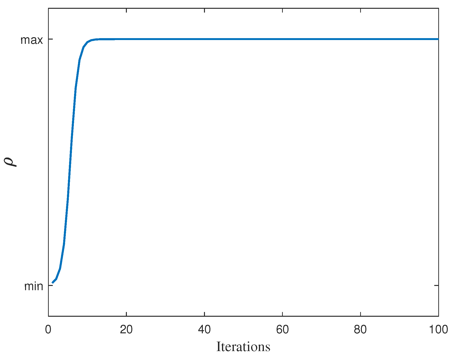
3.5. Variable Pheromone Evaporate Parameter
3.6. Modified Local Pheromone Update Rule
3.7. Algorithm Flow
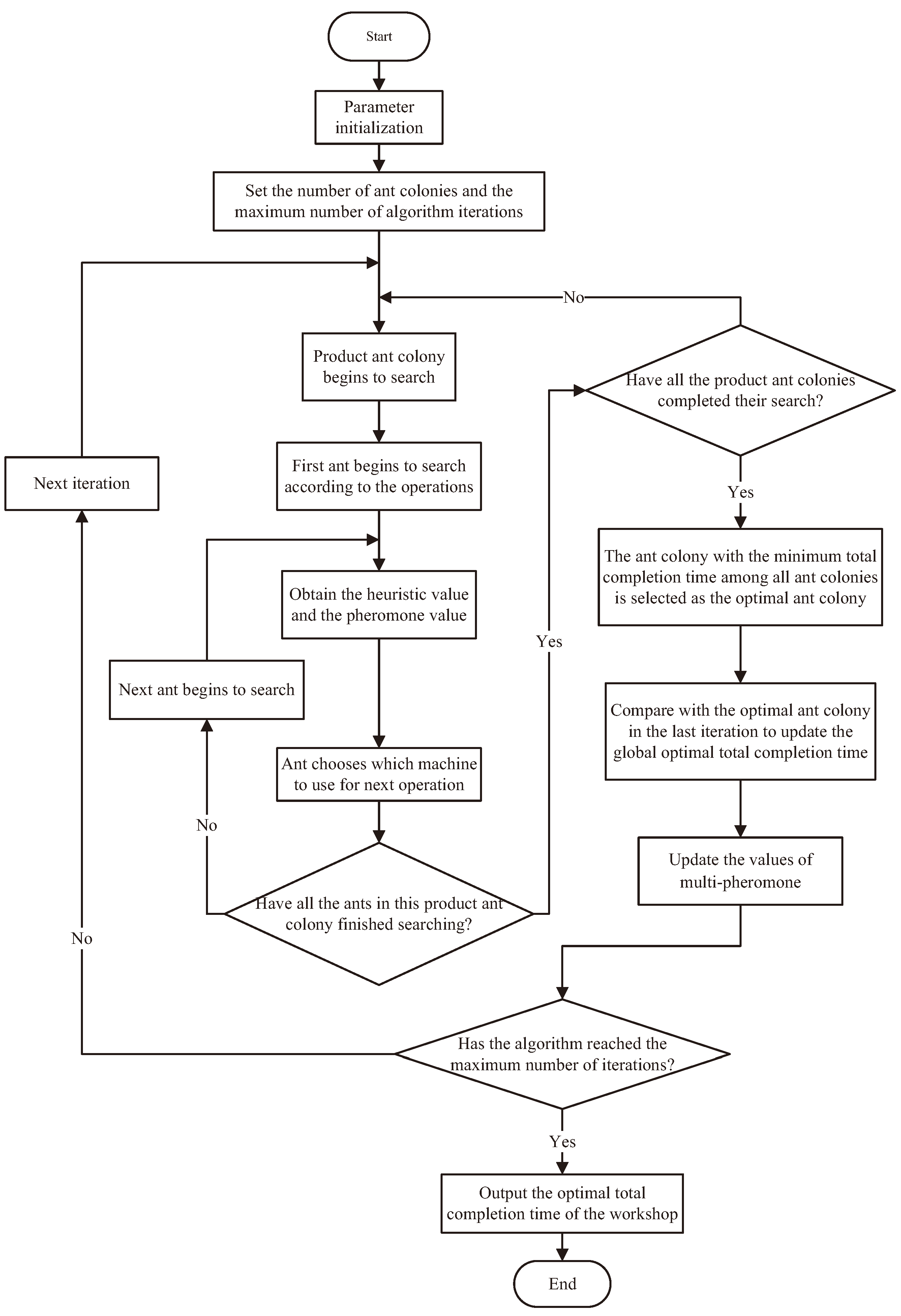
- Step 1:
- Initialize parameters of all operation machines and products (jobs). Initialize the number of product ant colonies and the maximum iteration number of the algorithm;
- Step 2:
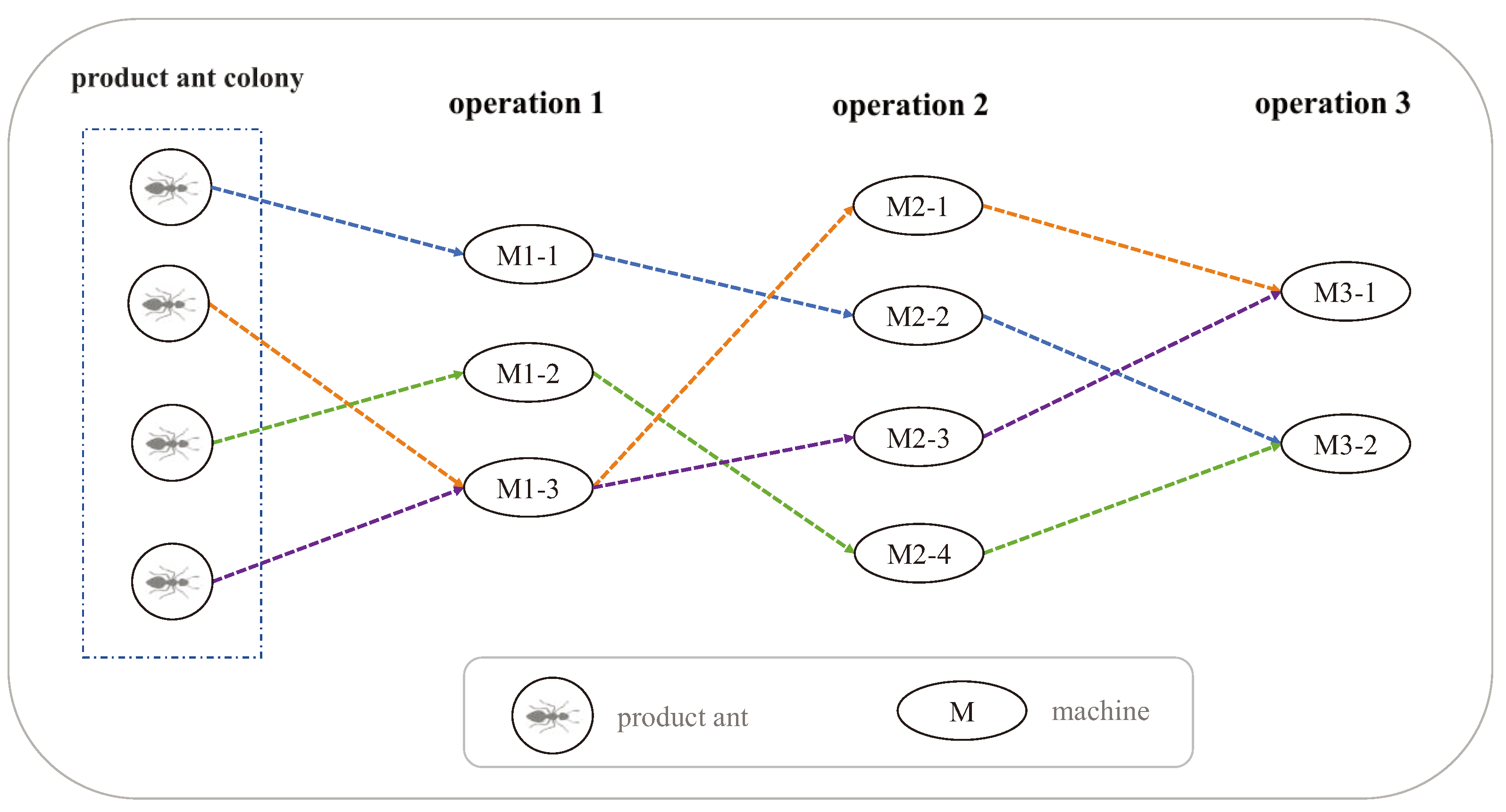
- The algorithm begins to iterate, and the first group of product ant colonies performs a machine search between each operation. The number of ants in each group of ant colonies corresponds to the number of textile products (jobs) to be produced in the workshop, and the corresponding number of pheromones is initialized accordingly;
- Step 3:
- Each ant in the ant colony calculates the heuristic values of each machine and the pheromone between machines to choose a route from the machine corresponding to one operation to the machine corresponding to the next operation;
- Step 4:
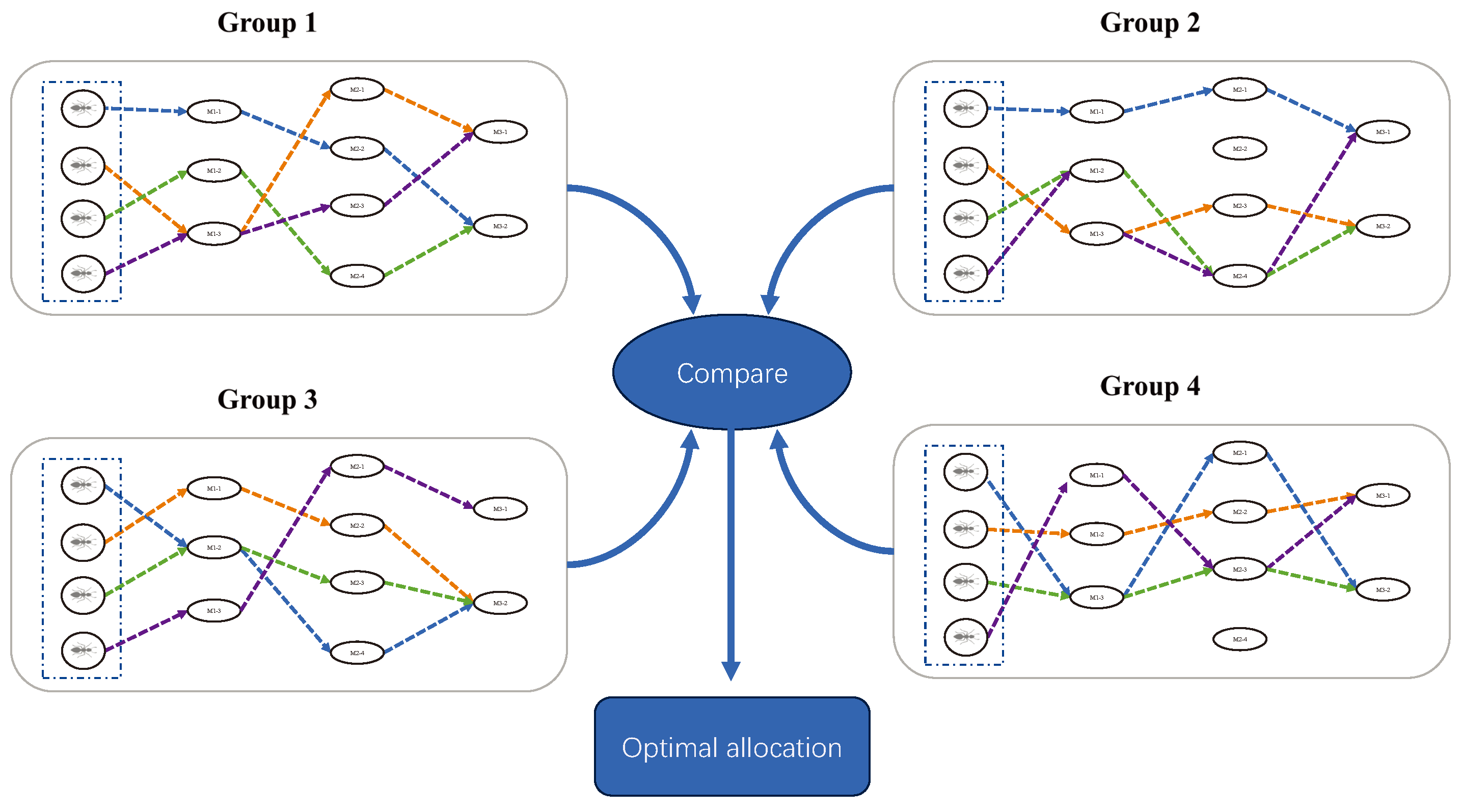
- The next colony begins its search. After all product ant colonies complete the search, the ant colony with the minimum is selected as the best ant colony and is compared with the optimal value of the last iteration, thereby updating the global optimal ant colony global multi-pheromone;
- Step 5:
- After the algorithm reaches the set maximum number of iterations, The of the algorithm is obtained.
4. Results and Analysis
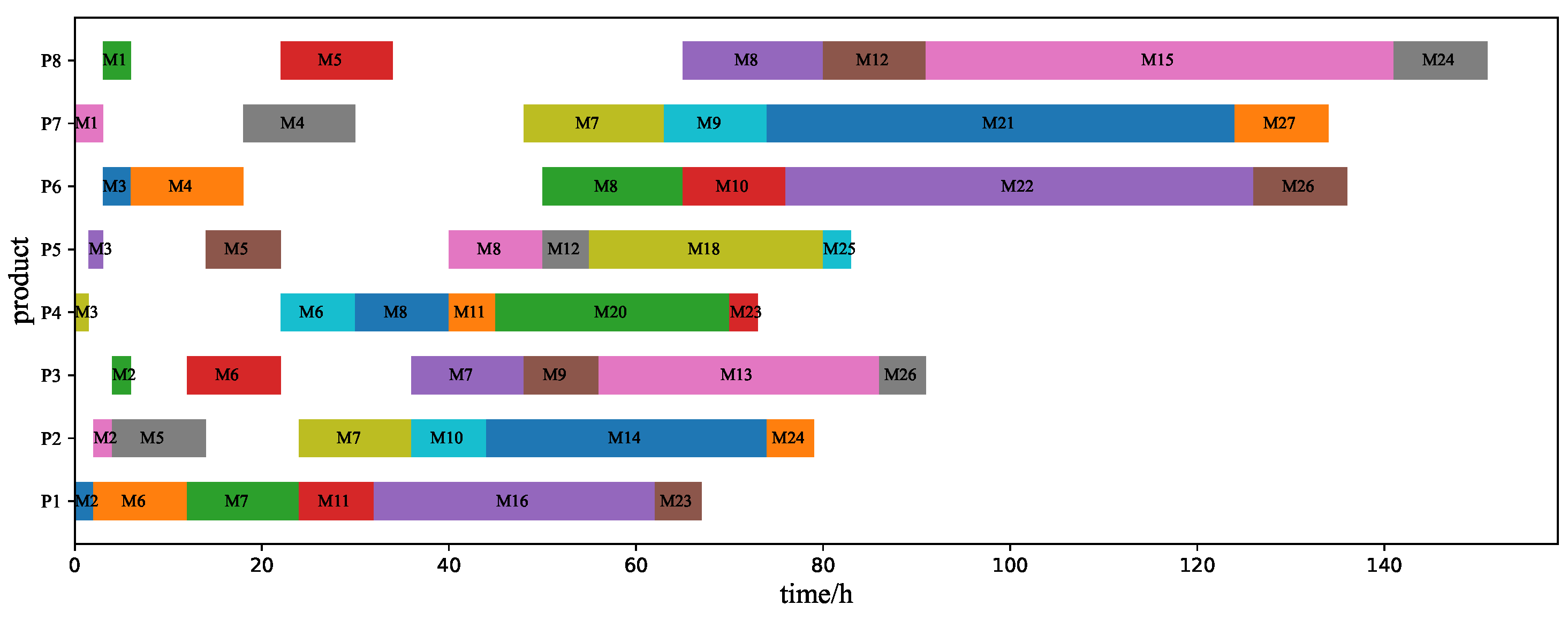
4.1. Simulation Model
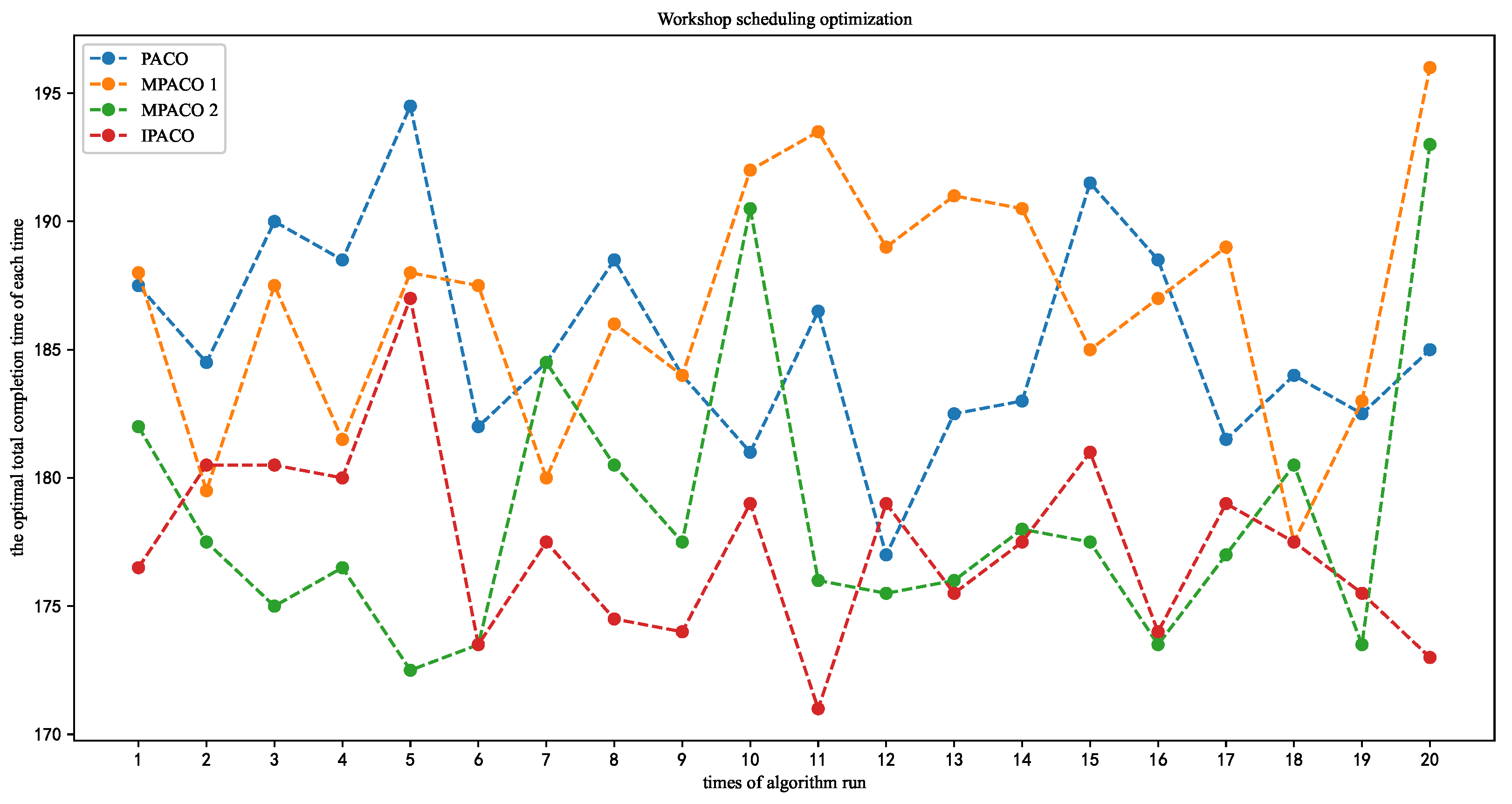
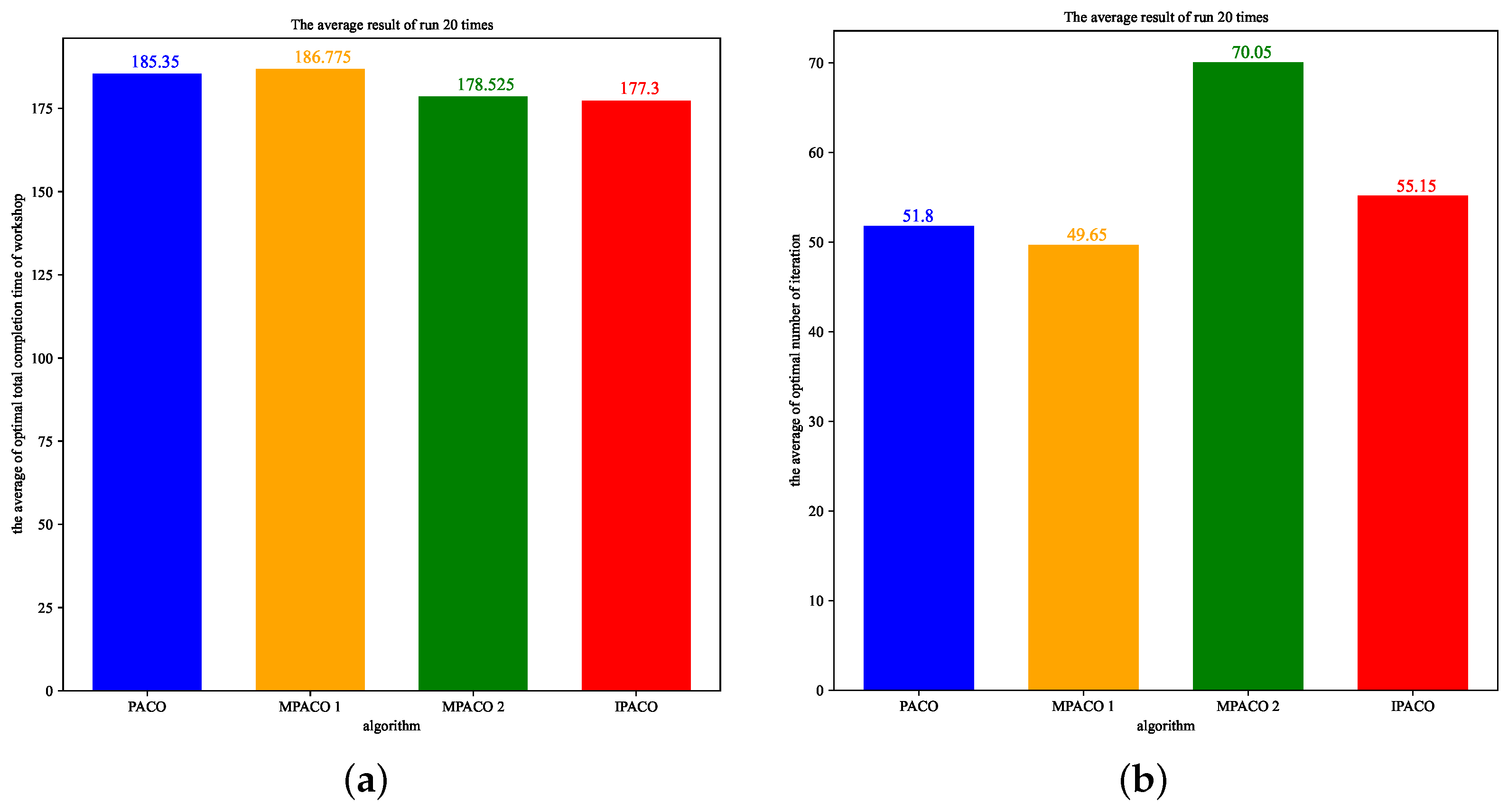
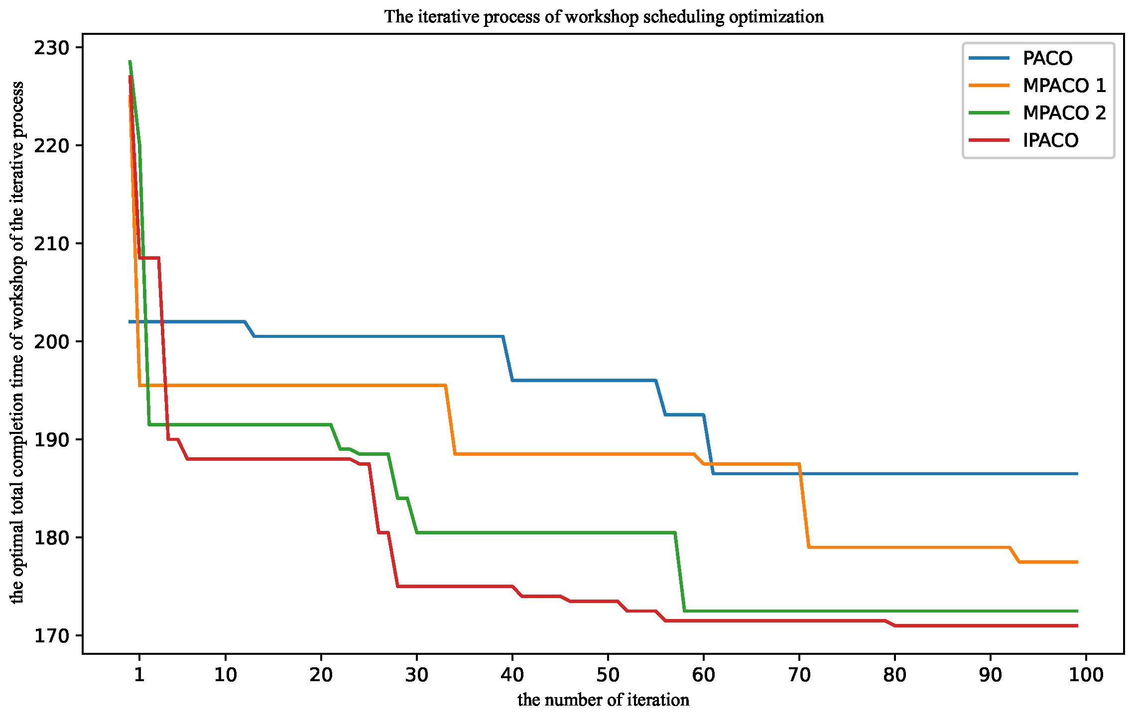
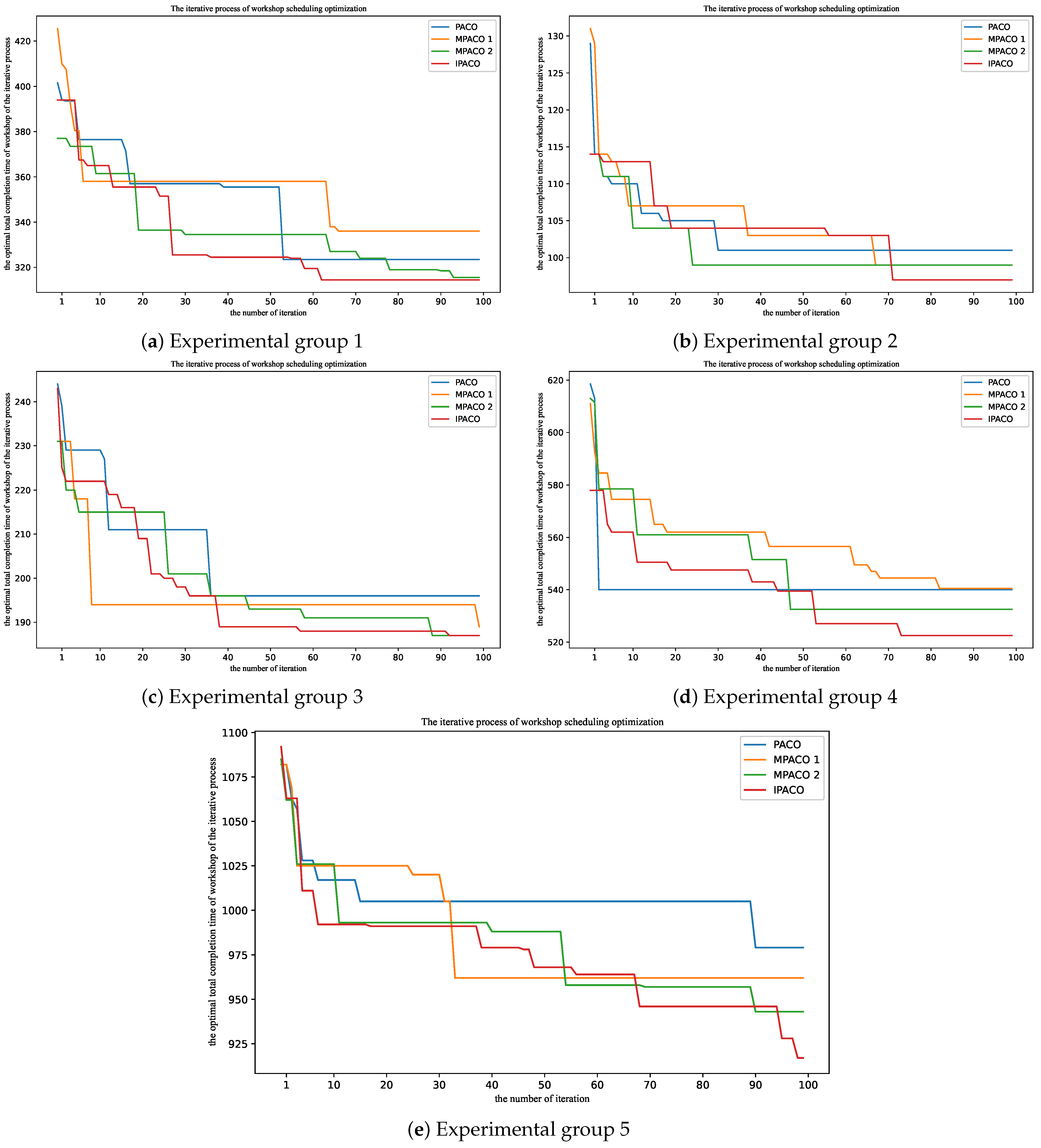
4.2. Modified PACO Algorithm Comparison
4.3. Comparative Analysis of Algorithms
4.4. Verification of Algorithms under Different Conditions
5. Conclusions
Author Contributions
Funding
Institutional Review Board Statement
Informed Consent Statement
Data Availability Statement
Conflicts of Interest
Abbreviations
| ACO | Ant Colony Optimization |
| PACO | Product Ant Colony Optimization |
| JSP | Job-shop Scheduling Problem |
| FJSP | Flexible Job-shop Scheduling Problem |
| LMEO | Learning-based Multipopulation Evolutionary Optimization |
| FJSP-Ts | Flexible Job-shop Scheduling Problem with finite Transportation resources |
| MILP | Mixed-Integer Linear Programming |
| OFA | Optimal Foraging Algorithm |
| PFS | Pythagorean Fuzzy Set |
| T-FJSP | Textile Flexible Job-shop Scheduling Problem |
| MPACO | Modified Product Ant Colony Optimization |
| IPACO | Integrated Product Ant Colony Optimization of MPACO 1 and MPACO 2 |
References
- Pan, R.; Zhang, N.; Xiang, J. Analysis of key technology and application status of textile intelligent factory. Cotton Text. Technol. 2023, 51, 105–110. [Google Scholar]
- Mei, S.; Hu, G.; Wang, J.; Chen, Z.; Xu, Q. Analysis of some key technology basis for intelligent textile manufacturing and its equipment. J. Text. Res. 2017, 38, 166–171. [Google Scholar]
- Zhou, J. Discussion on Feasibility of Weaving Enterprise to Realize Intelligent Production. Cotton Text. Technol. 2021, 49, 68–71. [Google Scholar]
- Ji, X. Discussion on Production Mode of Intelligent Weaving Factory. Cotton Text. Technol. 2020, 48, 75–78. [Google Scholar]
- Brucker, P.; Schlie, R. Job-shop scheduling with multi-purpose machines. Computing 1991, 45, 369–375. [Google Scholar] [CrossRef]
- Pan, Z.; Lei, D.; Wang, L. A Bi-Population Evolutionary Algorithm with Feedback for Energy-Efficient Fuzzy Flexible Job Shop Scheduling. IEEE Trans. Syst. Man Cybern. Syst. 2022, 52, 5295–5307. [Google Scholar] [CrossRef]
- Renna, P. Switch-Off Policies in Job Shop Controlled by Workload Control Concept. Appl. Sci. 2023, 13, 5210. [Google Scholar] [CrossRef]
- Pan, Z.; Wang, L.; Zheng, J.; Chen, J.F.; Wang, X. A Learning-Based Multipopulation Evolutionary Optimization for Flexible Job Shop Scheduling Problem with Finite Transportation Resources. IEEE Trans. Evol. Comput. 2023, 27, 1590–1603. [Google Scholar] [CrossRef]
- Fatemi-Anaraki, S.; Tavakkoli-Moghaddam, R.; Foumani, M.; Vahedi-Nouri, B. Scheduling of Multi-Robot Job Shop Systems in Dynamic Environments: Mixed-Integer Linear Programming and Constraint Programming Approaches. Omega 2023, 115, 102770. [Google Scholar] [CrossRef]
- Gaiardelli, S.; Carra, D.; Spellini, S.; Fummi, F. Dynamic Job and Conveyor-Based Transport Joint Scheduling in Flexible Manufacturing Systems. Appl. Sci. 2024, 14, 3026. [Google Scholar] [CrossRef]
- Kong, J.; Wang, Z. Research on Flexible Job Shop Scheduling Problem with Handling and Setup Time Based on Improved Discrete Particle Swarm Algorithm. Appl. Sci. 2024, 14, 2586. [Google Scholar] [CrossRef]
- Wang, H.J.; Zhu, G.Y. Multiobjective Optimization for FJSP Under Immediate Predecessor Constraints Based OFA and Pythagorean Fuzzy Set. IEEE Trans. Fuzzy Syst. 2023, 31, 3108–3120. [Google Scholar] [CrossRef]
- Liang, X.; Chen, J.; Gu, X.; Huang, M. Improved Adaptive Non-Dominated Sorting Genetic Algorithm with Elite Strategy for Solving Multi-Objective Flexible Job-Shop Scheduling Problem. IEEE Access 2021, 9, 106352–106362. [Google Scholar] [CrossRef]
- Ning, G.; Cao, D. Multi-step Genetic Algorithm for Solving Dynamic Flexible Job Shop Scheduling Problem. In Proceedings of the 2021 IEEE International Conference on Advances in Electrical Engineering and Computer Applications (AEECA), Dalian, China, 27–28 August 2021; pp. 23–28. [Google Scholar]
- Zhang, F.; Mei, Y.; Nguyen, S.; Zhang, M. Evolving Scheduling Heuristics via Genetic Programming with Feature Selection in Dynamic Flexible Job-Shop Scheduling. IEEE Trans. Cybern. 2021, 51, 1797–1811. [Google Scholar] [CrossRef]
- Dorigo, M.; Gambardella, L. Ant colony system: A cooperative learning approach to the traveling salesman problem. IEEE Trans. Evol. Comput. 1997, 1, 53–66. [Google Scholar] [CrossRef]
- Xu, D.S.; Ai, X.Y.; Xing, L.N. An Improved Ant Colony Optimization for Flexible Job Shop Scheduling Problems. In Proceedings of the International Joint Conference on Computational Sciences & Optimization, Sanya, China, 24–26 April 2009. [Google Scholar]
- Anitha, J.; Karpagam, M. Ant colony optimization using pheromone updating strategy to solve job shop scheduling. In Proceedings of the 2013 7th International Conference on Intelligent Systems and Control (ISCO), Tamil Nadu, India, 4–5 January 2013; pp. 367–372. [Google Scholar]
- Wang, L.; Cai, J.; Li, M.; Liu, Z. Flexible Job Shop Scheduling Problem Using an Improved Ant Colony Optimization. Sci. Program. 2017, 2017, 9016303. [Google Scholar] [CrossRef]
- Zhang, S.; Li, X.; Zhang, B.; Wang, S. Multi-objective optimisation in flexible assembly job shop scheduling using a distributed ant colony system. Eur. J. Oper. Res. 2020, 283, 441–460. [Google Scholar] [CrossRef]
- Miao, C.; Chen, G.; Yan, C.; Wu, Y. Path planning optimization of indoor mobile robot based on adaptive ant colony algorithm. Comput. Ind. Eng. 2021, 156, 107230. [Google Scholar] [CrossRef]
- Yang, X.; Xiong, N.; Xiang, Y.; Du, M.; Zhou, X.; Liu, Y. Path Planning of Mobile Robot Based on Adaptive Ant Colony Optimization. In Proceedings of the IECON 2021—47th Annual Conference of the IEEE Industrial Electronics Society, Toronto, ON, Canada, 13–16 October 2021; pp. 1–4. [Google Scholar]
- Jia, Y.H.; Mei, Y.; Zhang, M. A Bilevel Ant Colony Optimization Algorithm for Capacitated Electric Vehicle Routing Problem. IEEE Trans. Cybern. 2022, 52, 10855–10868. [Google Scholar] [CrossRef]
- Lei, D.; Li, M.; Wang, L. A Two-Phase Meta-Heuristic for Multiobjective Flexible Job Shop Scheduling Problem with Total Energy Consumption Threshold. IEEE Trans. Cybern. 2019, 49, 1097–1109. [Google Scholar] [CrossRef]
- Zhang, G. Research on Methods for Flexible Job Shop Scheduling Problems. Ph.D. Thesis, Huazhong University of Science and Technology, Wuhan, China, 2011. [Google Scholar]
- Li, R.; Gong, W.; Lu, C.; Wang, L. A Learning-Based Memetic Algorithm for Energy-Efficient Flexible Job-Shop Scheduling with Type-2 Fuzzy Processing Time. IEEE Trans. Evol. Comput. 2023, 27, 610–620. [Google Scholar] [CrossRef]
- Dorigo, M.; Gambardella, L.M. Ant colonies for the travelling salesman problem. Biosystems 1997, 43, 73–81. [Google Scholar] [CrossRef] [PubMed]
- Mavrovouniotis, M.; Müller, F.M.; Yang, S. Ant Colony Optimization with Local Search for Dynamic Traveling Salesman Problems. IEEE Trans. Cybern. 2017, 47, 1743–1756. [Google Scholar] [CrossRef] [PubMed]
- Li, J.; Deng, H.; Liu, D.; Song, C.; Han, R.; Hu, T. A Job Shop Scheduling Method Based on Ant Colony Algorithm. In Proceedings of the 2021 IEEE International Conference on Progress in Informatics and Computing (PIC), Shanghai, China, 17–19 December 2021; pp. 453–457. [Google Scholar]
- Mao, W.; Li, S.; Xie, X.; Yang, X.; Nie, J. Global path planning of mobile robot based on adaptive mechanism improved ant colony algorithm. Control. Decis. 2023, 38, 2520–2528. [Google Scholar]
- Wei, D.; Zhang, X.; Hu, M. Joint Task Allocation Method Based on Multi-pheromone Ant Colony Algorithm. J. China Acad. Electron. Inf. Technol. 2019, 14, 798–807+812. [Google Scholar]
- Zheng, P.; Zhang, P.; Wang, M.; Zhang, J. A Data-Driven Robust Scheduling Method Integrating Particle Swarm Optimization Algorithm with Kernel-Based Estimation. Appl. Sci. 2021, 11, 5333. [Google Scholar] [CrossRef]


| Symbol | Meaning | Symbol | Meaning |
|---|---|---|---|
| n | Total textile products (jobs) | The operating completion time of operation h of job j | |
| m | Total machines | The operating completion time of operation h of job j on machine i | |
| Machine index, | The number of machines that can be selected for operation h of job j | ||
| Job index, | L | A large positive number | |
| The total operations of job j | The completion time of each textile product (job) | ||
| Operation index, | The makespan of the textile workshop | ||
| The operation h of job j | The total machine operating time of machine i | ||
| The operation h of job j processed on machine i | The total production time of textile product (job) | ||
| The operating time of operation h of job j processed on machine i | T | The total completion time of the workshop | |
| The operating start time of operation h of job j | The optimal total completion time of the workshop |
| Machine ID | Operation | Number of Machines |
|---|---|---|
| M1~M3 | yarn hanging | 3 |
| M4~M6 | beam warping | 3 |
| M7~M8 | warp sizing | 2 |
| M9~M12 | looming | 4 |
| M13~M22 | weaving | 10 |
| M23~M27 | packaging | 5 |
| Product ID | Product Category | Yarn Hanging | Beam Warping | Warp Sizing | Looming | Weaving | Packaging | Product Number |
|---|---|---|---|---|---|---|---|---|
| P1~P3 | Product 1 | 2 | 10 | 12 | 8 | 30 | 5 | 3 |
| P4~P5 | Product 2 | 1.5 | 8 | 10 | 5 | 25 | 3 | 2 |
| P6~P8 | Product 3 | 3 | 12 | 15 | 11 | 50 | 10 | 3 |
| Algorithm | Q | |||||
|---|---|---|---|---|---|---|
| PACO | 1 | 5 | 0.3 | 10 | 0 | |
| MPACO 1 | 1 | 5 | 0.25 | 0.45 | 10 | 0 |
| MPACO 2 | 1 | 5 | 0.3 | 10 | 0.2 | |
| IPACO | 1 | 5 | 0.25 | 0.45 | 10 | 0.2 |
| PACO | MPACO 1 | MPACO 2 | IPACO | |||||
|---|---|---|---|---|---|---|---|---|
| Time (h) | Iteration | Time (h) | Iteration | Time (h) | Iteration | Time (h) | Iteration | |
| 1 | 184.5 | 60 | 183 | 34 | 182 | 90 | 176.5 | 29 |
| 2 | 186 | 44 | 183.5 | 99 | 177.5 | 53 | 180.5 | 91 |
| 3 | 182.5 | 12 | 193.5 | 5 | 175 | 47 | 180.5 | 95 |
| 4 | 184.5 | 86 | 192 | 8 | 176.5 | 87 | 180 | 38 |
| 5 | 188.5 | 41 | 188 | 73 | 172.5 | 59 | 187 | 24 |
| 6 | 188.5 | 73 | 182 | 97 | 173.5 | 79 | 173.5 | 40 |
| 7 | 190 | 69 | 192.5 | 29 | 184.5 | 100 | 177.5 | 60 |
| 8 | 184 | 60 | 192.5 | 61 | 180.5 | 62 | 174.5 | 49 |
| 9 | 185.5 | 89 | 182.5 | 6 | 177.5 | 75 | 174 | 51 |
| 10 | 188 | 84 | 188 | 39 | 190.5 | 78 | 179 | 60 |
| 11 | 181.5 | 72 | 184.5 | 16 | 176 | 20 | 171 | 81 |
| 12 | 182.5 | 68 | 190 | 12 | 175.5 | 99 | 179 | 51 |
| 13 | 184 | 47 | 184 | 62 | 176 | 95 | 175.5 | 53 |
| 14 | 197 | 70 | 179 | 41 | 178 | 67 | 177.5 | 74 |
| 15 | 193 | 25 | 181 | 79 | 177.5 | 95 | 181 | 50 |
| 16 | 187.5 | 26 | 184 | 60 | 173.5 | 75 | 174 | 45 |
| 17 | 188.5 | 91 | 188 | 25 | 177 | 46 | 179 | 46 |
| 18 | 186.5 | 96 | 178 | 28 | 180.5 | 98 | 177.5 | 20 |
| 19 | 188 | 23 | 184 | 13 | 173.5 | 72 | 175.5 | 82 |
| 20 | 189 | 78 | 187.5 | 67 | 193 | 4 | 173 | 64 |
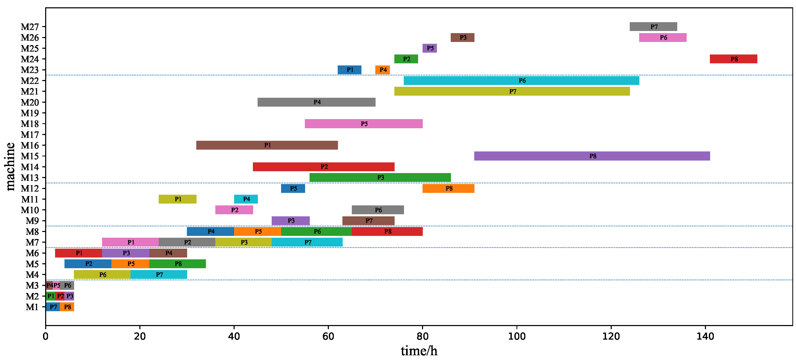
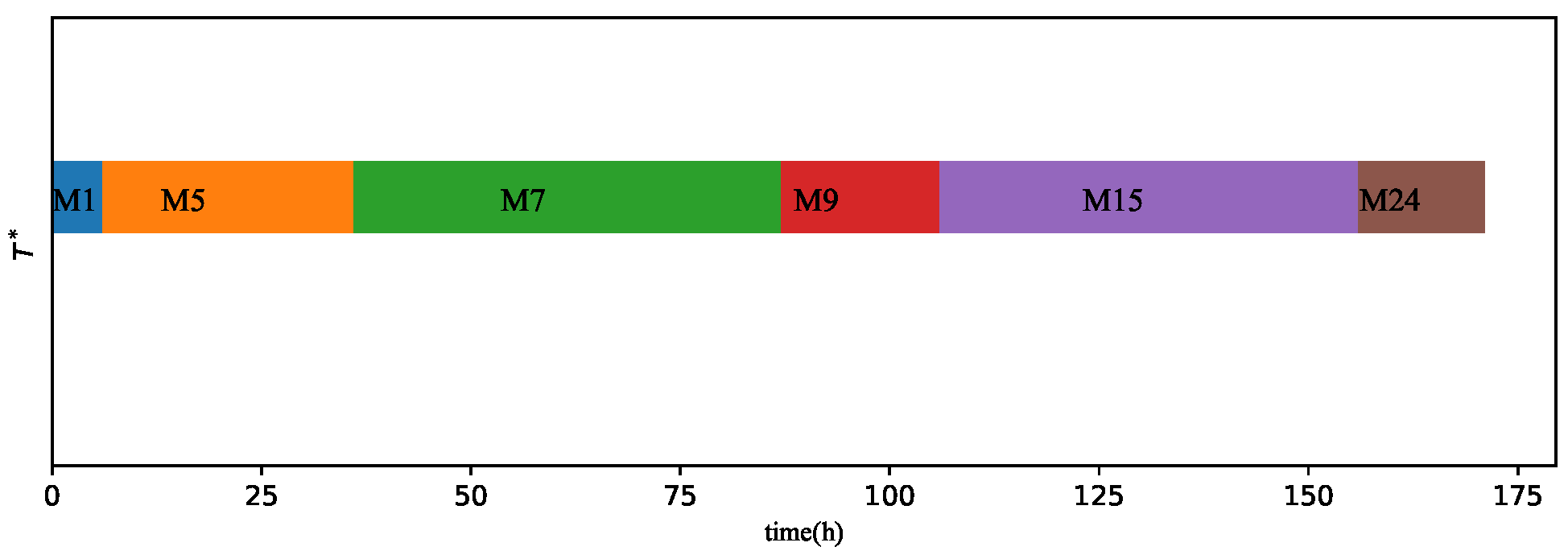
| Machine | The Process of Machine | Total Operating Time (h) | Machine | The Process of Machine | Total Operating Time (h) |
|---|---|---|---|---|---|
| M1 | 6 | M15 | 50 | ||
| M2 | 6 | M16 | 30 | ||
| M3 | 6 | M17 | × | 0 | |
| M4 | 24 | M18 | 25 | ||
| M5 | 30 | M19 | × | 0 | |
| M6 | 28 | M20 | 25 | ||
| M7 | 51 | M21 | 50 | ||
| M8 | 50 | M22 | 50 | ||
| M9 | 19 | M23 | 8 | ||
| M10 | 19 | M24 | 15 | ||
| M11 | 13 | M25 | 3 | ||
| M12 | 16 | M26 | 15 | ||
| M13 | 30 | M27 | 10 | ||
| M14 | 30 |
| Operation | Number of Machines Corresponding to the Operation (Total Number of Operations) | ||||
|---|---|---|---|---|---|
| Group 1 (6) | Group 2 (4) | Group 3 (5) | Group 4 (7) | Group 5 (8) | |
| Operation 1 | 3 | 3 | 4 | 5 | 2 |
| Operation 2 | 3 | 4 | 4 | 2 | 4 |
| Operation 3 | 2 | 5 | 2 | 6 | 3 |
| Operation 4 | 4 | 3 | 5 | 3 | 2 |
| Operation 5 | 10 | 0 | 3 | 2 | 5 |
| Operation 6 | 5 | 0 | 0 | 3 | 6 |
| Operation 7 | 0 | 0 | 0 | 2 | 6 |
| Operation 8 | 0 | 0 | 0 | 0 | 4 |
| Quantity of Products | Product | Operation | ||||||||
|---|---|---|---|---|---|---|---|---|---|---|
| Oper. 1 | Oper. 2 | Oper. 3 | Oper. 4 | Oper. 5 | Oper. 6 | Oper. 7 | Oper. 8 | |||
| Group 1 | 5 | Product 1 | 2 | 10 | 12 | 8 | 30 | 5 | 0 | 0 |
| 5 | Product 2 | 1.5 | 8 | 10 | 5 | 25 | 3 | 0 | 0 | |
| 5 | Product 3 | 3 | 12 | 15 | 11 | 50 | 10 | 0 | 0 | |
| Group 2 | 4 | Product 1 | 5 | 3 | 8 | 13 | 0 | 0 | 0 | 0 |
| 6 | Product 2 | 7 | 2 | 12 | 11 | 0 | 0 | 0 | 0 | |
| Group 3 | 3 | Product 1 | 9 | 10 | 6 | 32 | 3 | 0 | 0 | 0 |
| 2 | Product 2 | 12 | 12 | 7 | 24 | 3 | 0 | 0 | 0 | |
| 3 | Product 3 | 10 | 14 | 10 | 35 | 5 | 0 | 0 | 0 | |
| 2 | Product 4 | 7 | 13 | 9 | 28 | 4 | 0 | 0 | 0 | |
| Group 4 | 2 | Product 1 | 15 | 20 | 5 | 16 | 13 | 2 | 10 | 0 |
| 4 | Product 2 | 13 | 28 | 7 | 15 | 15 | 3 | 13 | 0 | |
| 3 | Product 3 | 12.5 | 23 | 5 | 11 | 20 | 2 | 12 | 0 | |
| 2 | Product 4 | 14 | 26 | 6 | 14 | 20 | 3 | 10 | 0 | |
| 3 | Product 5 | 13 | 19 | 7 | 17 | 18 | 3 | 14 | 0 | |
| Group 5 | 8 | Product 1 | 25 | 14 | 21 | 30 | 5 | 8 | 19 | 21 |
| 10 | Product 2 | 20 | 16 | 19 | 36 | 7 | 6 | 19 | 20 | |
| Algorithm | (%) | (%) | |||
|---|---|---|---|---|---|
| Group 1 | PACO | 348.225 | 6.24 | 323.5 | 2.86 |
| MACO 1 | 348.775 | 6.41 | 336 | 6.84 | |
| MACO 2 | 331.225 | 1.05 | 315.5 | 0.32 | |
| IPACO | 327.775 | 0 | 314.5 | 0 | |
| Group 2 | PACO | 104.85 | 3.45 | 101 | 4.12 |
| MACO 1 | 103.35 | 1.97 | 99 | 2.06 | |
| MACO 2 | 102.1 | 0.74 | 99 | 2.06 | |
| IPACO | 101.35 | 0 | 97 | 0 | |
| Group 3 | PACO | 203 | 5.65 | 196 | 4.81 |
| MACO 1 | 200.85 | 4.53 | 189 | 1.07 | |
| MACO 2 | 194.15 | 1.04 | 187 | 0 | |
| IPACO | 192.15 | 0 | 187 | 0 | |
| Group 4 | PACO | 551.825 | 2.55 | 540 | 3.35 |
| MACO 1 | 552.6 | 2.69 | 540.5 | 3.44 | |
| MACO 2 | 540.3 | 0.4 | 529 | 1.24 | |
| IPACO | 538.125 | 0 | 522.5 | 0 | |
| Group 5 | PACO | 997.5 | 4.9 | 979 | 6.76 |
| MACO 1 | 991.55 | 4.27 | 962 | 4.91 | |
| MACO 2 | 957.35 | 0.67 | 943 | 2.84 | |
| IPACO | 950.95 | 0 | 917 | 0 |
Disclaimer/Publisher’s Note: The statements, opinions and data contained in all publications are solely those of the individual author(s) and contributor(s) and not of MDPI and/or the editor(s). MDPI and/or the editor(s) disclaim responsibility for any injury to people or property resulting from any ideas, methods, instructions or products referred to in the content. |
© 2024 by the authors. Licensee MDPI, Basel, Switzerland. This article is an open access article distributed under the terms and conditions of the Creative Commons Attribution (CC BY) license (https://creativecommons.org/licenses/by/4.0/).
Share and Cite
Chen, F.; Xie, W.; Ma, J.; Chen, J.; Wang, X. Textile Flexible Job-Shop Scheduling Based on a Modified Ant Colony Optimization Algorithm. Appl. Sci. 2024, 14, 4082. https://doi.org/10.3390/app14104082
Chen F, Xie W, Ma J, Chen J, Wang X. Textile Flexible Job-Shop Scheduling Based on a Modified Ant Colony Optimization Algorithm. Applied Sciences. 2024; 14(10):4082. https://doi.org/10.3390/app14104082
Chicago/Turabian StyleChen, Fengyu, Wei Xie, Jiachen Ma, Jun Chen, and Xiaoli Wang. 2024. "Textile Flexible Job-Shop Scheduling Based on a Modified Ant Colony Optimization Algorithm" Applied Sciences 14, no. 10: 4082. https://doi.org/10.3390/app14104082
APA StyleChen, F., Xie, W., Ma, J., Chen, J., & Wang, X. (2024). Textile Flexible Job-Shop Scheduling Based on a Modified Ant Colony Optimization Algorithm. Applied Sciences, 14(10), 4082. https://doi.org/10.3390/app14104082