Article

GNSS-Assisted Visual Dynamic Localization Method in Unknown Environments

1
School of Aerospace Engineering, Zhengzhou University of Aeronautics, Zhengzhou 450001, China
2
Institute of Geospatial Information, Information Engineering University, Zhengzhou 450001, China
3
Henan General Aviation Engineering Technology Research Centre, Zhengzhou 450001, China
*
Author to whom correspondence should be addressed.
Appl. Sci. 2024, 14(1), 455; https://doi.org/10.3390/app14010455
Submission received: 24 October 2023 / Revised: 22 November 2023 / Accepted: 24 November 2023 / Published: 4 January 2024

Abstract

:
Autonomous navigation and localization are the foundations of unmanned intelligent systems, therefore, continuous, stable, and reliable position services in unknown environments are especially important for autonomous navigation and localization. Aiming at the problem where GNSS cannot continuously localize in complex environments due to weak signals, poor penetration ability, and susceptibility to interference and that visual navigation and localization are only relative, this paper proposes a GNSS-aided visual dynamic localization method that can provide global localization services in unknown environments. Taking the three frames of images and their corresponding GNSS coordinates as the constraint data, the GNSS coordinate system and world coordinate system transformation matrix are obtained through horn coordinate transformation, and the relative positions of the subsequent image sequences in the world coordinate system are obtained through epipolar geometry constraints, homography matrix transformations, and 2D–3D position and orientation solving, which ultimately yields the global position data of unmanned carriers in GNSS coordinate systems when GNSS is temporarily unavailable. Both the dataset validation and measured data validation showed that the GNSS initial-assisted positioning algorithm could be applied to situations where intermittent GNSS signals exist, and it can provide global positioning coordinates with high positioning accuracy in a short period of time; however, the algorithm would drift when used for a long period of time. We further compared the errors of the GNSS initial-assisted positioning and GNSS continuous-assisted positioning systems, and the results showed that the accuracy of the GNSS continuous-assisted positioning system was two to three times better than that of the GNSS initial-assisted positioning system, which proved that the GNSS continuous-assisted positioning algorithm could maintain positioning accuracy for a long time and it had good reliability and applicability in unknown environments.

1. Introduction

Existing satellite positioning and navigation systems such as GPS (Global Positioning System), GLONASS (Global Orbiting Navigation Satellite System), BDS (Beidou Navigation Satellite System), Galileo (Galileo Satellite Navigation System), QZSS (Japanese Quasi-Zenith Satellite Navigation System), and IRNSS (Indian Regional Satellite Navigation System), together with corresponding ground-based and satellite-based augmentation systems, comprise the infrastructure for global PNT (positioning, navigation, and timing) services [1,2]. The development of satellite navigation and positioning systems have changed people’s ways of life, the styles of battlefield perception, and the modes of traffic management, which has promoted the development of science and technology, economies, and societies. However, at the same time, satellite positioning and navigation systems have natural vulnerabilities, such as weak signals, poor penetration abilities, and susceptibility to interference [3]. In some complex environments, such as urban canyons, tunnels, or battlefields with strong interference, GNSS (Global Navigation Satellite System) signals are weakened or even rejected, which causes the position information obtained by the GNSS receiver to be unavailable, and thus, it is necessary to rely on other navigation methods (e.g., Wi-Fi [4], UWB (ultra-wide band) [5], 3D LiDAR and vision [6], etc.) to obtain reliable global position coordinates.
Visual navigation and localization comprise a passive and reliable localization model [7] that can realize autonomous navigation and localization in a location environment after acquiring video or image sequences, and visual navigation and localization have the advantages of possessing anti-interference abilities, being capable of high accuracy, and being low cost, and so they are widely used in the field of autonomous intelligence [8]. However, the state estimation positions obtained by visual localization are relative, it is difficult to determine the global position of a carrier, and there is a drift phenomenon in the long-term localization of a visual navigation error.
Two navigation and localization methods, GNSS and vision, have their own advantages and disadvantages, and they can form complementary advantages [9,10]. GNSS can inhibit the rapid accumulation of visual navigation errors, and visual navigation can achieve continuous navigation when GNSS is subjected to occlusion and interference, which improves the navigation and localization continuity and accuracy of GNSS.
There are many experts and scholars that have conducted GNSS and visual navigation research. For example, in the literature, the authors of [11] utilized GNSS as an external absolute positioning system to provide scale information for monocular visual odometers, and this assisted the visual odometers used for navigation and positioning.
There have been more studies on GNSS and vision for loose combinations of navigation and localization. Agrawal and Konolige [12] firstly proposed a GNSS/VO loose combination system which used a cart equipped with a GNSS receiver and a binocular camera for experiments, and they confirmed that the performance of the GNSS/VO loose combination system was better than that of a pure visual VO system. Aumayer et al. [13] investigated the performance of a binocular-vision-assisted GNSS for continuous navigation in harsh environments, and it loosely combined pure visual navigation results with GNSS results. The experiments showed that when the GNSS accuracy was reduced to 10 m in a weak GNSS environment, the accuracy of the visual navigation results was better than 1 m, and so the visual navigation system could well assist the GNSS for continuous navigation.
In addition, Schreiber et al. [14] used a tightly combined GNSS/inertial system which utilized pseudo-ranging or carrier-phase raw observations, and the final experiments proved that when the number of satellites was less than four, the tightly combined localization solution could still be carried out. Wang Lei et al. [15] proposed that the feature points in images with known world coordinate systems were regarded as “visual pseudo-satellites”, and they could be tightly combined with GNSS ranging signals to realize continuous navigation in weak GNSS environments. In the literature, the authors of [16,17] utilized a tight combination in the case of insufficient satellite observations to carry out navigation research on a combined GNSS and vision system.
In conclusion, there have been more studies related to the combination and assistance of vision and GNSS. However, most of these studies were based on vision/GNSS loosely coupled or tightly coupled in general frameworks, and this required GNSS signals to be present for a long time to be used for navigation and localization; therefore, these are not applicable to cases where GNSS is not available or only opportunistic signals are present. To address the above problems, we used intermittently available GNSS positioning results as constraint data to assist with vision for localization, realizing that the global position of an unmanned carrier can still be obtained when GNSS data are not available.
Specifically, we made the following contributions: we proposed a general framework for GNSS-assisted visual dynamic localization, stating that the overall process consisted of five parts (initialization, a GNSS coordinate system and world coordinate system conversion, frame sequence tracking and position and orientation estimation, local optimization, and frame sequence GNSS coordinate-solving).
We took three frames of images and their corresponding GNSS coordinates as the constraint data, and we calculated the transformation matrix between the GNSS coordinate system and the world coordinate system through the Horn coordinate transformation. Then, the relative position and orientation relations of the image sequence in the world coordinate system could be obtained using epipolar geometry constraints, homography transformation, PNP (perspective-n-point) positions, and orientation solving. Finally, the position parameters of the carrier in the GNSS coordinate system under the GNSS rejection were obtained.
We validated this study’s algorithm based on a dataset and the measured data, respectively. The validation results showed that the algorithm was applicable to the case of the presence of intermittent GNSS opportunity signals, and it could provide global position services with high short-term positioning accuracy. However, due to the scale drift of the visual odometer itself, this algorithm was not applicable to the case of complete GNSS signal rejection when the visual localization results could not be constrained and corrected. Then, we further compared the errors of the GNSS initial-assisted positioning and GNSS continuous-assisted positioning, and the results showed that the accuracy of the GNSS continuous-assisted positioning was two to three times higher than that of the GNSS initial-assisted positioning, which proved that the GNSS continuous-assisted positioning algorithm could maintain positioning accuracy for a long time, and it had good reliability and applicability in unknown environments.
The rest of this paper is organized as follows. The framework of the GNSS-assisted visual dynamic positioning method is given in Section 2. In Section 3, the algorithm flow is established, including initialization, the GNSS coordinate system, the world coordinate system conversion, the frame sequence tracking and position and orientation estimation, the local optimization, and the frame sequence GNSS coordinate-solving. In Section 4, through dataset validation, the applicability of this paper’s algorithm is demonstrated. In Section 5, through discussing our experiments with real data, it is further verified that the GNSS continuous-assisted algorithm improved the accuracy by a factor of two to three with respect to the GNSS initial-assisted algorithm. Finally, conclusions and further research arrangements are drawn in Section 6.

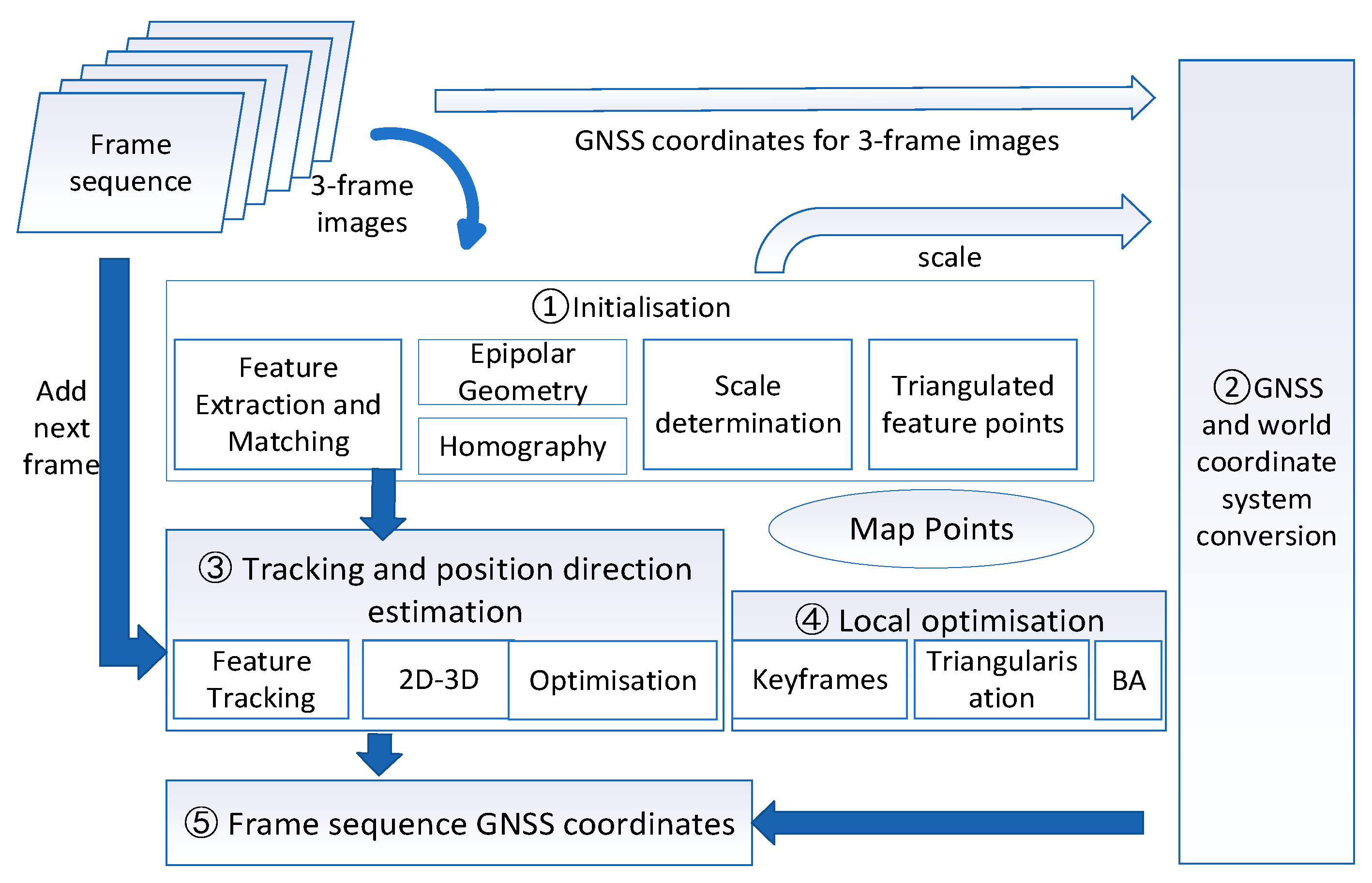
2. GNSS-Assisted Visual Dynamic Localization Method Framework
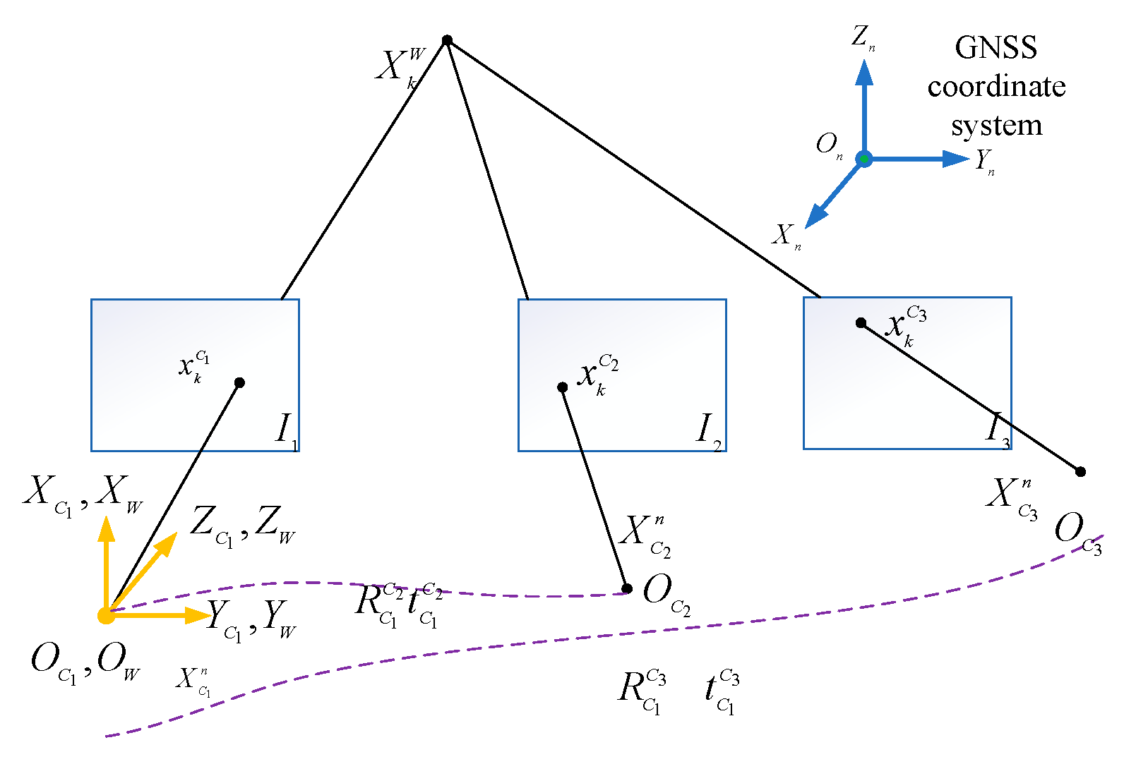
In this study, three frames of images and their corresponding GNSS coordinates were used as constraint data, and the transformation matrix between the GNSS coordinate system and the world coordinate system (the camera coordinate system of the first frame of the image was used as the world coordinate system) was computed using the Horn coordinate transformation [18]. The relative positions and orientations of the subsequent image sequences in the world coordinate system were obtained through epipolar geometry constraints [19], homography transformation [19], and a 2D–3D positional solution model. Combining the GNSS coordinate system and the world coordinate system transformation matrix, the position data of the carrier in the GNSS coordinate system when GNSS was not available were finally obtained. Figure 1 shows the overall process framework, illustrating that the overall process consisted of the following five parts: initialization, the GNSS coordinate system and world coordinate system conversion, tracking and position-solving, local optimization, and the GNSS coordinate-solving for the frame sequences.

2.1. Initialization

Initialization is the process of obtaining a position estimation from the first three frames of an image, and it includes feature extraction and matching, relative position-solving with epipolar geometry constraints and a homography matrix, and, finally, triangulated feature points.
As Figure 2 shows, I 1 , I 2 , and I 3 were three frames of an image with GNSS positioning data, and their corresponding camera photocenter positions were C 1 , C 2 , and C 3 , while the GNSS coordinates were X C 1 n , X C 2 n , and X C 3 n . Here, the camera coordinate system O C 1 X C 1 Y C 1 Z C 1 at C 1 was assumed to be the world coordinate system O W X W Y W Z W .

2.1.1. Positional Solution Using Epipolar Geometry Constraints

Orb feature point extraction and matching were performed for I 1 , I 2 , and I 3 to obtain matching homonymous points. Taking the k-th homonymous point as an example, the normalized coordinates of the pixels in I 1 , I 2 , and I 3 were noted as x k C 1 , x k C 2 , and x k C 3 .
The following constraints were established based on the pair of epipolar geometry equations, as (1) shows below:
x k C 2 T E C 1 C 2 x k C 1 = 0   and   E C 2 C 1 = K T F C 2 C 1 K = [ t C 2 C 1 ] × R C 2 C 1 ,
where E C 2 C 1 represents the essential matrix from I 1 to I 2 , F C 2 C 1 represents the fundamental matrix from I 1 to I 2 , R C 2 C 1 represents the rotation matrix from the movement of C 1 to C 2 , and t C 2 C 1 represents the translation vector from the movement of C 1 to C 2 .
The SVD decomposition was performed on the essential matrix E C 2 C 1 to obtain the four combinations corresponding to R C 2 C 1 , t C 2 C 1 . Usually, any point can be substituted to determine the depth of a point, and when the constraint that the feature point needs to be in front of the camera is utilized, the only correct result of the pose to solve R C 2 C 1 , t C 2 C 1 is selected.

2.1.2. Positional Solving Using a Homography Matrix

If the homonymous points are in the same plane, then the positional solution can be performed according to the homography matrix, as (2) shows below:
x k C 2 = H C 1 C 2 x k C 1
where H C 1 C 2 denotes the homography matrix from I 1 to I 2 .
The SVD decomposition of the homography matrix H C 1 C 2 is performed as follows in (3):
H C 1 C 2 = U D V T   and   D = R D + t D n D T d ,
where U and V are orthogonal matrices and D is a diagonal matrix.
Here, the SVD decomposition was performed with D as the new single response matrix, and R C 2 C 1 and t C 2 C 1 under the single response relation could be obtained.

2.1.3. Model Scores

R C 2 C 1 = U R D V T ,   n = V n D ,   t C 2 C 1 = d U t D
The epipolar geometry constraint and homography matrix were introduced as (4) shows above. In a real scenario, it is necessary to judge which model to choose for a positional solution according to the distribution of feature points in a shooting scene.
Here, we performed model scoring by judging the number of interior points. Equation (5) shows the defined ratio, and score H and score F represent the H matrix and F matrix scores, respectively:
r a t i o = s c o r e H s c o r e H + s c o r e F
Here, the ratio threshold was set to 0.6 based on the results of several experiments, and when the ratio was greater than 0.6, the homography matrix was selected for solving.

2.1.4. Scale Determinations

Although the above yielded the translation vector t C 2 C 1 , t C 2 C 1 was a translation vector that lost scale. According to the Euclidean transformation distance preserving property, the baseline length of the C 1 motion to C 2 in a GNSS coordinate system and the Euclidean distance of the translation vector of the C 1 motion to C 2 were equal; therefore, according to Equation (6), the scale factor λ 1 , 2 could be calculated as follows:
t C 2 C 1 = λ 2 , 1 X C 2 n X C 1 n
The real translation vector was as follows:
t C 2 C 1 = t C 2 C 1 / λ 2 , 1

2.1.5. Triangulation of the Feature Points

When two images are known to have the same name, matching point, and camera matrix, the 3D coordinates of the same name point can be solved. Here, using C 1 as the reference coordinate system, the camera matrices corresponding to I 1 and I 2 were as follows:
P 1 = K [ I | 0 ]   and   P 2 = K [ R C 2 C 1 | t C 2 C 1 ] .
Equation (8) was substituted into (9) to obtain the 3D coordinates, X k W , in the world coordinate system corresponding to the k-th feature point, as follows:
x k C 1 = P 1 X k W   and x k C 2 = P 2 X k W .
The least squares solution for the 3D coordinates X k W was obtained by solving the system of chi-square equations using SVD.

2.2. GNSS and World Coordinate System Conversion

According to the Horn absolute coordinate transformation, the rotation and translation transformation parameters between two Cartesian coordinate systems can be solved if there are three non-collinear coordinate points.
According to Equations (6) and (7), the real-scale translation vector for the movement of C 1 to C 3 could be obtained in the same way as (10), as follows:
t C 3 C 1 = t C 3 C 1 / λ 3 , 1
The GNSS coordinate system and the world coordinate system were both rigid-body coordinate systems, and so the transformation matrix consisted of the following two parts: the rotation vector R W n and the translation vector t W n . Here, the position X C 1 n of C 1 in the GNSS coordinate system was known to be the translation vector t W n , and the positions of C 2 and C 3 in the GNSS coordinate system were known to be X C 2 n and X C 3 n . The relation could then be jointly established using Equation (11), as follows:
X C 2 n = R W n t C 2 W + t W n   and   X C 3 n = R W n t C 3 W + t W n .
In addition, the rotation matrix R W n was a 3 * 3 orthogonal matrix that satisfied the following constraints:
R W n 1 T = 1 ,   R W n 2 T = 1 ,   and   R W n 3 T = 1 ,
where R W n 1 T , R W n 2 T , and R W n 3 T denote the first, second, and third column vectors of R W n , respectively.
The rotation vectors could be computed from the system by simultaneously using Equations (11) and (12). We noted that the three frames of the image constrained here were required to be sufficiently spatial, otherwise, a pathological transformation matrix would result.

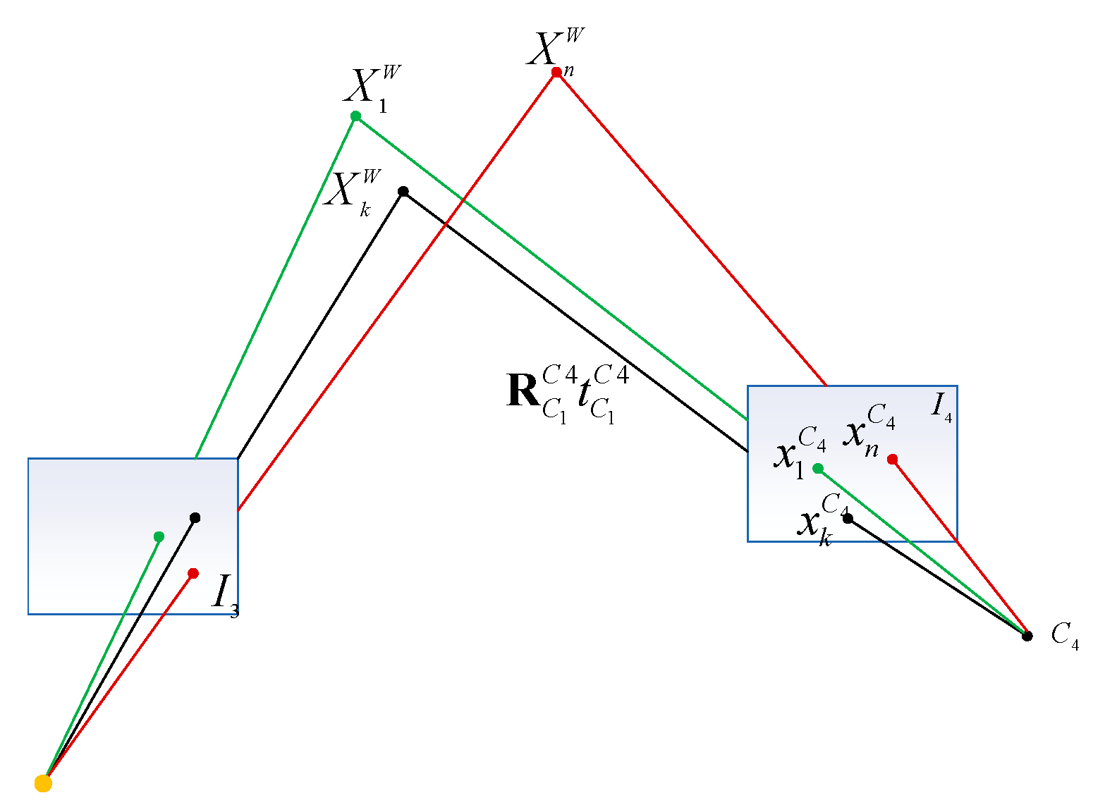
2.3. Subsequent Frame Sequence Tracking and Position-Solving

Here, the process of solving the algorithm for solving the subsequent image position was analyzed as an example of solving image I 4 . The following position-solving was carried out using a 2D–3D model.
As Figure 3 shows, it was assumed that I 4 and I 3 had matching points with the same name, and here, the position n and orientations R C 4 C 1 and t C 4 C 1 in the world coordinate system could be solved according to the RPNP algorithm. Then, R C 4 C 1 and t C 4 C 1 were further obtained using BA (bundle adjustment) optimization with the RPnP (robust perspective-n-point) [19,20] computed value as the initial value and the reprojection error as the objective function.
We defined the reprojection error as follows:
e = x P X   and 1 2 k = 1 n e k C 4 2 = 1 2 k = 1 n x k C 4 P 4 X k W 2 .
The P 4 optimal solution was selected by performing BA optimization using a reprojection error.

2.4. Local Optimization

The keyframe [21] was a representative one, and it needed to be selected with enough frames from the previous keyframe while being far enough away from the nearest keyframe. At the same time, it needed to have enough co-visual feature points in the local optimization. If the current frame was identified as a keyframe, a new 3D map point was created using that frame. In this phase, the camera pose and 3D map points were adjusted by constraining the minimization of the reprojection error, i.e., by using local optimization.
Using the itch frame camera poses, R C i C 1 and t C i C 1 , corresponding to the camera matrix P i , there were a total of m frames of images in the local map. The n map points corresponding to frame i were X 1 W , , X n W . The reprojection error was as follows (14):
e = x P X   and 1 2 i = 1 m j = 1 n e i j 2 = 1 2 i = 1 m j = 1 n x i j P i X j W 2 .

2.5. Subsequent Frame Sequence GNSS Coordinate-Solving

When the position of the subsequent image in the world coordinate system was obtained, the GNSS coordinates of the subsequent sequence of frames could be obtained by solving jointly with R W n . The following equation took I 4 as an example, and it solved the position of C 4 in the GNSS coordinate system as follows:
X C 4 n = X C 1 n + R W n t C 4 C 1

3. The Overall Flow of the Algorithm

Based on the sorting and deduction of the above related contents, an overall framework diagram and the implementation steps of the visual dynamic positioning algorithm flow with GNSS assistance were created, as Figure 4 and Table 1 show.

4. Dataset Validation

We validated the algorithm using the TUM dataset [22], which is a dataset of indoor and outdoor images collected by the Computer Vision Group of Ludwig Maximilian University. The dataset contains calibration files, five types of data, and the real trajectory of the camera captured by the motion-capture system. The true values of the motion capture system were used instead of the GNSS data to validate the visual dynamic localization method with GNSS assistance proposed in this paper. To verify the performance of the algorithms for the GNSS continuous aid and GNSS initial aid, three frames of the GNSS coordinates were randomly added for the constraints after the 78th frame. Table 2 shows the TUM dataset camera parameters.

4.1. Data Processing and Analysis

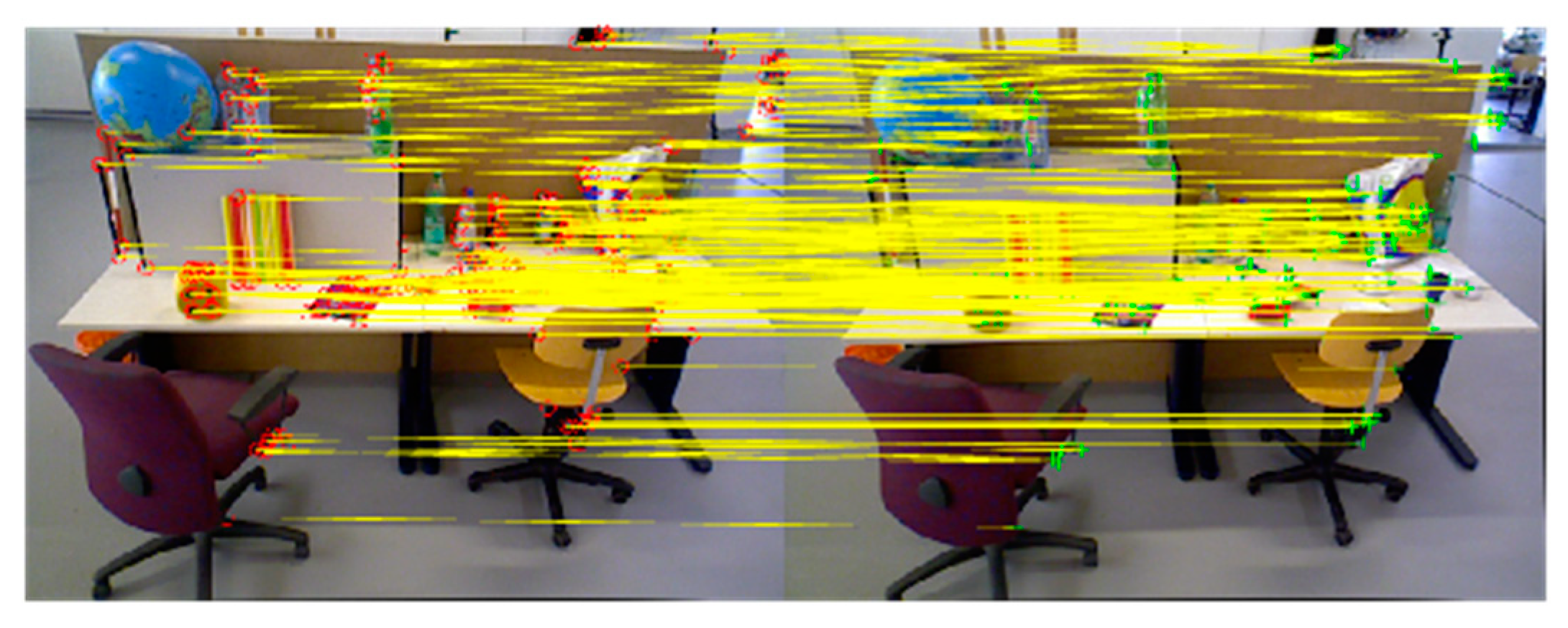
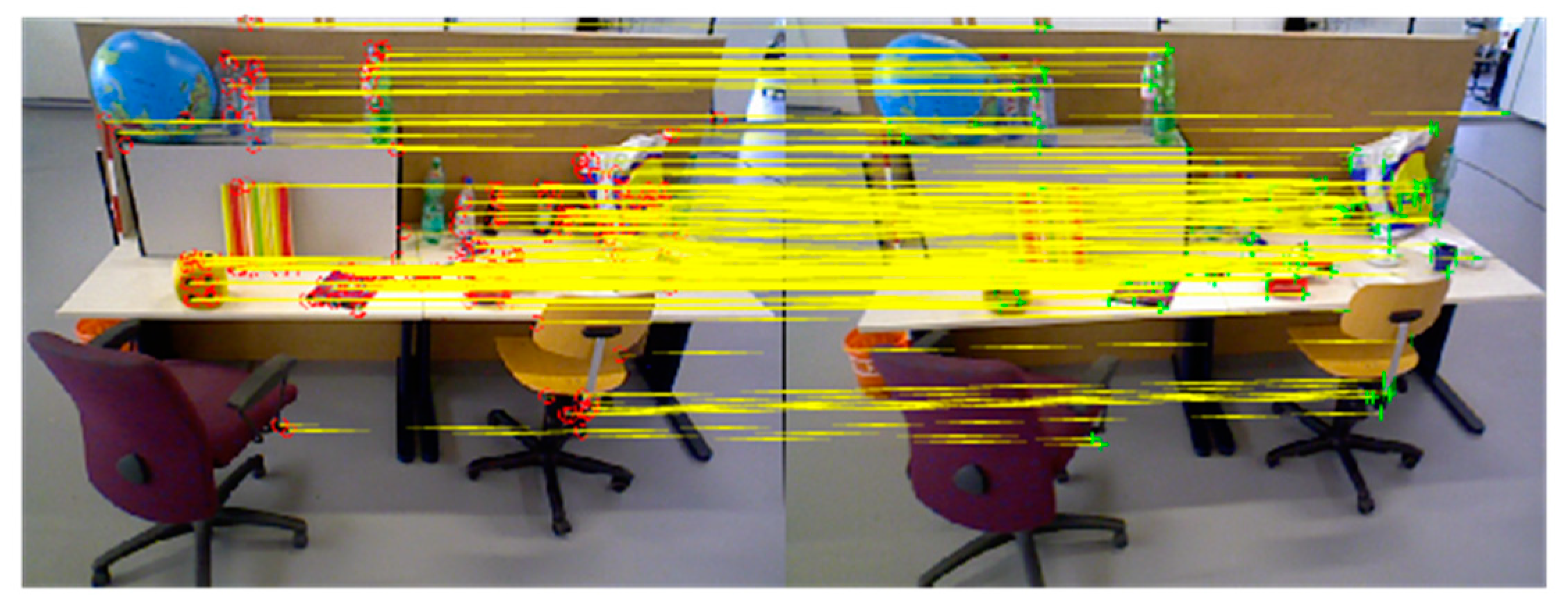
4.1.1. Feature Extraction and Matching

Frame 1, Frame 2, and Frame 3 were extracted orb feature points, and this setup involved an eight-layer image pyramid on the extraction of the FAST corner points, with a pyramid scale factor of 1.2. In this image, the resolution was 640 * 480, and we chose to extract 1000 corner points, as Figure 5 shows.
For the orb feature descriptor for the Frame 1 and Frame 2 feature point matching, a total of 253 pairs of matching points were obtained, as Figure 6 shows. Frame 1 and Frame 3 were matched, and a total of 211 pairs of feature points were obtained, as Figure 7 shows.

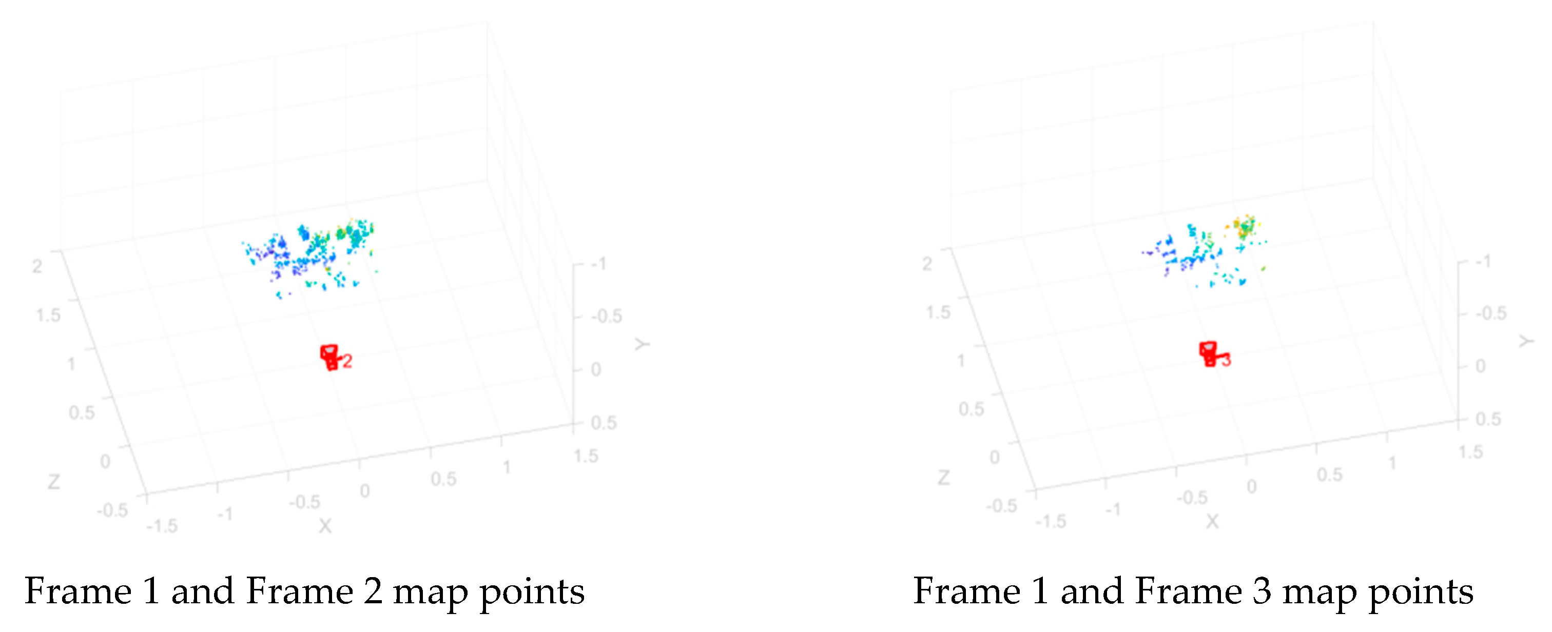
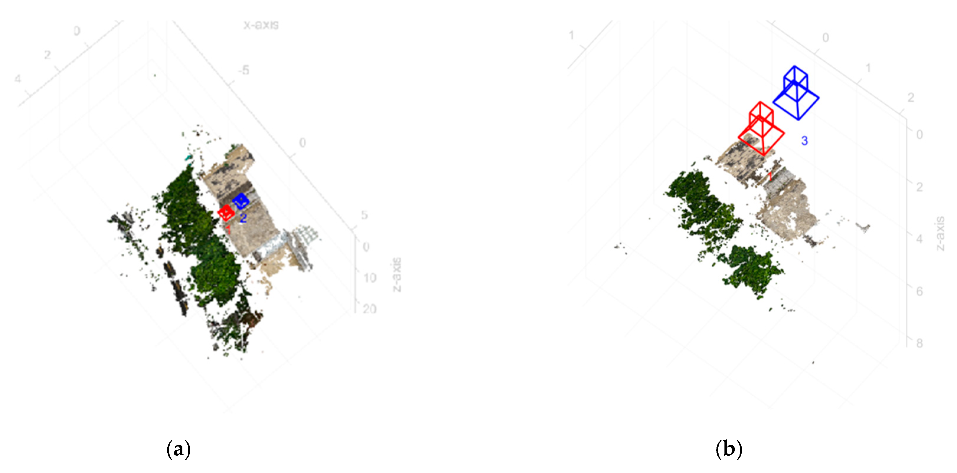
4.1.2. Triangulation

Frames 1 and 2 and Frames 1 and 3 were triangulated to obtain the corresponding map points. Table 3 shows the specific data processing results.
After triangulation, the map points were obtained, as Figure 8 shows. In the figure, the position of the camera and the map points in the camera’s view are labeled.

4.1.3. Motion Capture Coordinate System and World Coordinate System Transformation Matrix

In accordance with Section 2.2, the transformation matrix between the motion capture coordinate system and the world coordinate system were solved as follows:
R W n = 0 0 1.0000 0.4721 0.8815 0 0.8815 0.4721 0

4.1.4. Subsequent Camera Poses

For the subsequent frames, after tracking and local optimization, the corresponding camera poses were sequentially obtained in terms of position and attitude in the motion capture coordinate system, as Figure 9 shows. The red meter sign indicates the GNSS initial-aided positioning for the subsequent frame position, the blue circle indicates the GNSS continuous-assisted positioning for the subsequent frame position, and the green asterisk indicates the real pose data.
As Figure 9 shows, at the beginning stage, the GNSS initial-aided positioning trajectory, the GNSS continuous-assisted trajectory, and the true trajectory were nearly the same, which proved the effectiveness of the proposed method. However, with the passage of time, the GNSS initial-aided positioning trajectory appeared to drift obviously compared with the GNSS continuous-assisted trajectory. This was because for the GNSS initial auxiliary trajectory, the global position constraint was only effective at the beginning, and the overall accuracy degradation problem was subsequently manifested due to the accumulation of errors in the visual odometer itself.

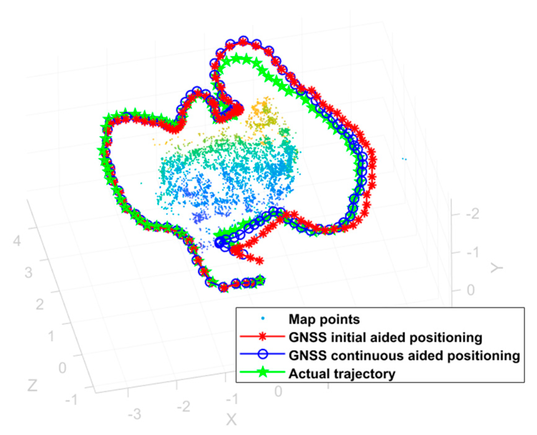
4.2. Error Statistics and Analysis

An absolute error analysis of the GNSS initial-aided positioning trajectory and the GNSS continuous-assisted trajectory with respect to the true trajectories was carried out. As Figure 10 shows, the red meter sign indicates the GNSS initial-aided positioning error and the blue circle indicates the GNSS continuous-assisted error. Overall, the x, y, and z axis errors appeared to increase with the number of frames, but the GNSS continuous-assisted error had a decreasing trend relative to the GNSS initial-aided positioning error.
Here, a further statistical analysis of the GNSS initial-aided positioning error accuracy and the GNSS initial-aided positioning error accuracy was carried out. The mean absolute error (MAE) was defined as follows:
M A E = i = 1 n x C i G N S S x C i G N S S t r u t h n
where x C i G N S S t r u t h represents the true value of the GNSS coordinates of the camera center in frame i.
To analyze the applicability of the GNSS-aided visual dynamic localization method proposed in this study, Table 4 shows the following statistics for the different frame numbers’ (20, 70, 100, and 143) MAEs.
As Table 4 shows, from Frame 4 to Frame 20 and then to Frame 70, the mean absolute errors and root mean square errors increased, but the overall error increased slowly. However, for GNSS initial-aided positioning, from 70 frames, and especially after 100 frames, the error increased exponentially. For the GNSS continuous-aided positioning, the error growth was slow, and compared with the GNSS initial-aided positioning error, the accuracy was improved by two to three times. The proposed algorithm could provide stable and continuous global location services.

5. Experiments with Real Data

To further verify the effectiveness of the algorithm in this study, the following real-scene measured data were used for the algorithm verification. Here, a DJI M300 (It is manufactured in China by Shenzhen DJI Innovation Technology Co., Shenzhen, China) aircraft was used, and it was equipped with a Searle camera with five lenses (front, back, left, right, and down) and a high-precision PPK. The location of the collected image data is the north gate of the Zhengzhou University of Aeronautics, and the aircraft flew at a constant speed, collecting a total of 414 * 5 images and outputting the corresponding high-precision GNSS position of each image at the same time.
In this experiment, the downward-looking lens image was the experimental data, and of the 414 images collected, for the images with high-precision position labeling, Figure 11a shows the trajectory below. The captured images could be 3D-reconstructed for tilt photogrammetry, and the airborne 3D measurement was calculated using Context Capture, as Figure 11b shows.
In the following algorithm validation, the starting three frames of the image GNSS coordinates were used as the initial constraints, and three frames of the image GNSS coordinates were added as the continuous constraints at every subsequent interval of 35 frames.

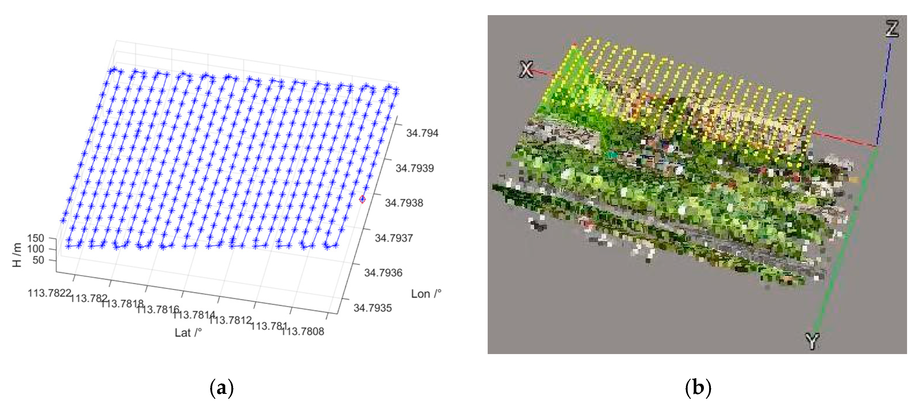
5.1. Data Processing

5.1.1. Camera Calibration

In this study, the Camera Calibrator toolbox [23] in MATLAB was used by Zhang Zheng for the checkerboard grid calibration, and the internal reference matrix was obtained as follows:
6377.341875 0 2994 . 3 0 4251 . 56125 1978 . 42 0 0 0
The distortion parameter was as follows:
[ 0.03484541 0.06374797 0.01231441 0.00002336 0.00036276 ]
The overall error in calibration did not exceed 0.7 pixels, and the average error did not exceed 0.4 pixels.

5.1.2. Image Distortion Processing

The original image was distorted using calibrated internal parameters, and Figure 12 shows the partially de-distorted image, where the left side is the original image and the right side is the de-distorted image.

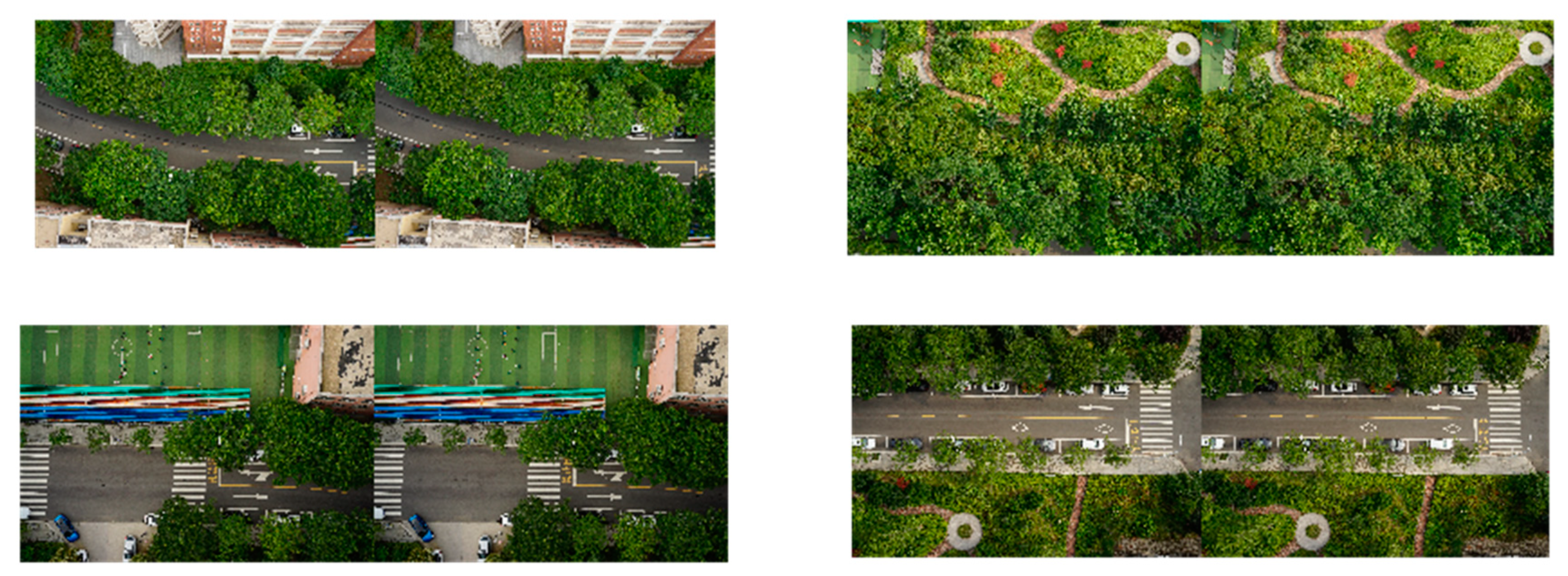
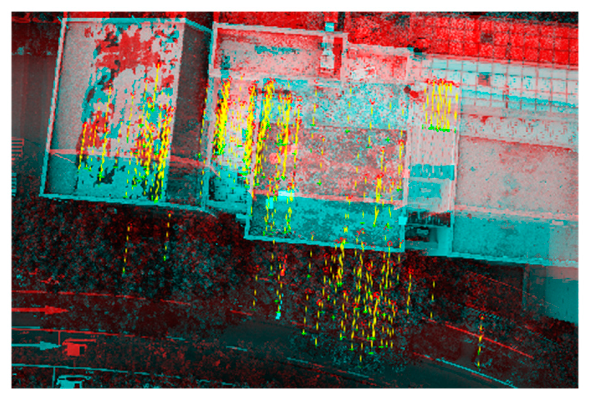
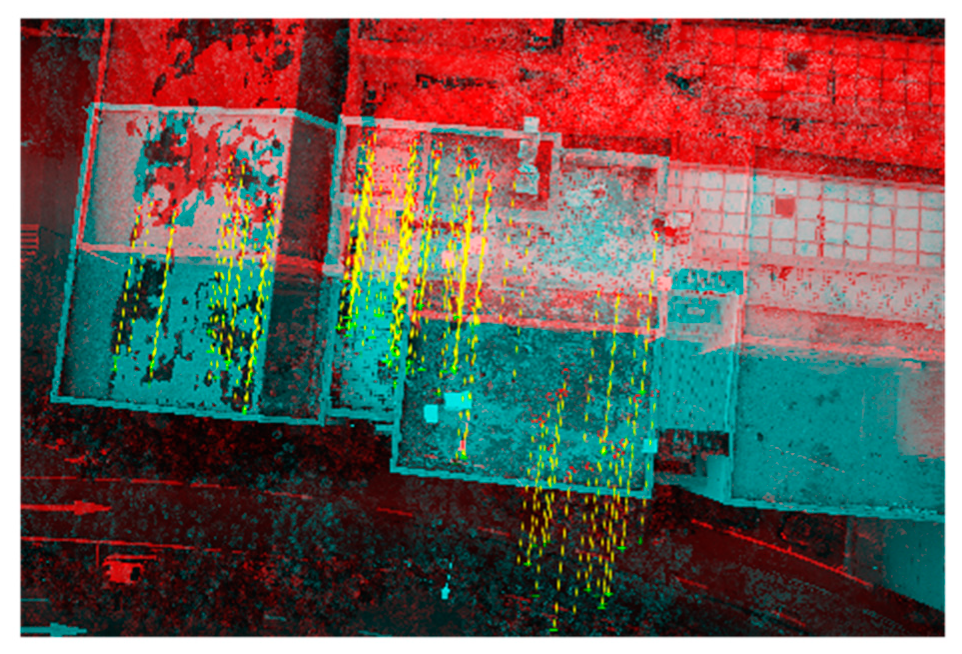
5.1.3. Feature Point Extraction and Matching

The orb feature descriptor was used to match the Frame 1 and Frame 2 feature points, and a total of 563 pairs of matching points were obtained. For Frame 1 and Frame 3, a total of 458 pairs of feature points were obtained, as Figure 13 and Figure 14 show.
The points of Frames 1 and 2 and Frames 1 and 3 were triangulated to obtain the corresponding map points, as Figure 15 shows.

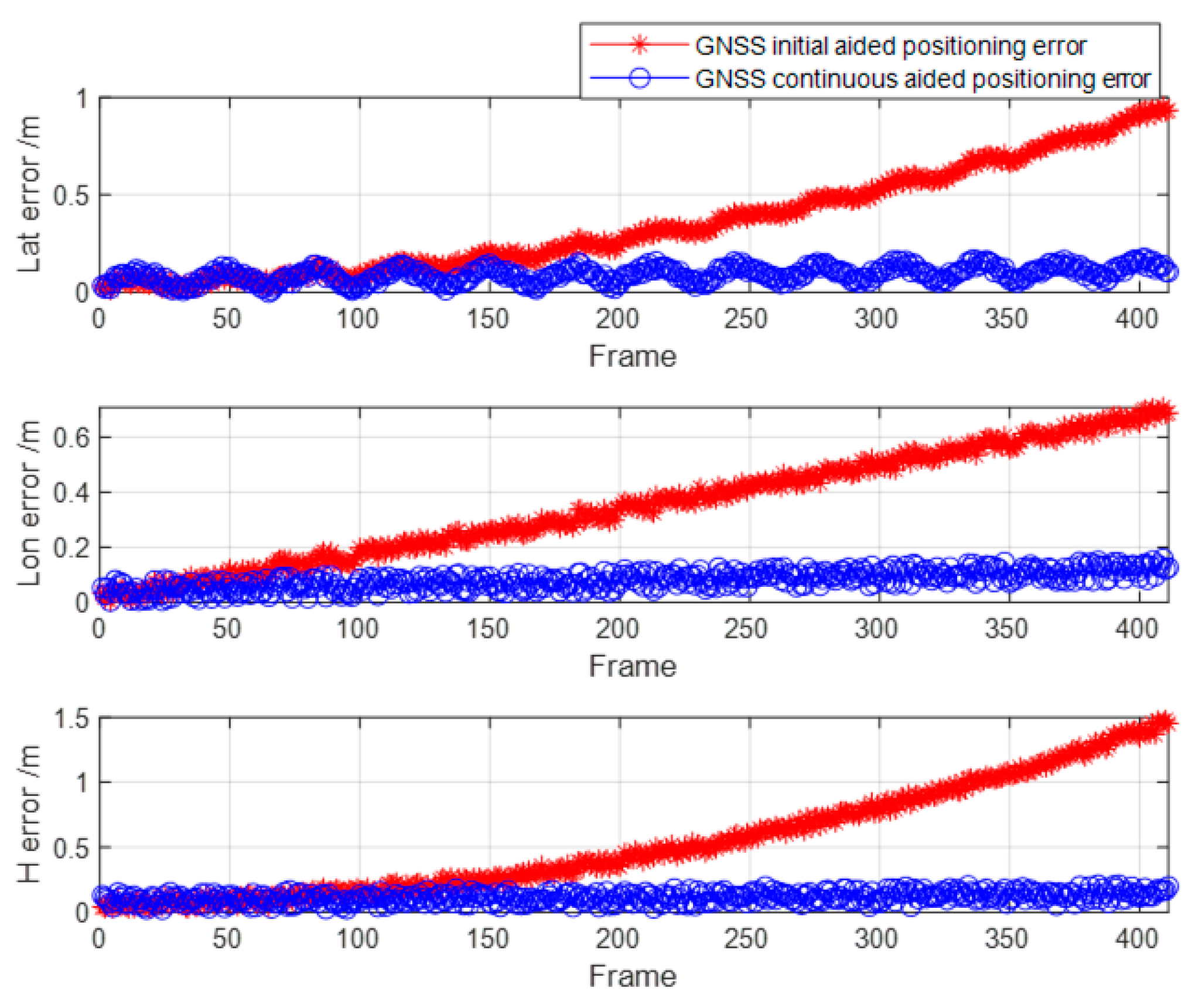
5.2. Error Statistics and Analysis

After the global position of the frame was obtained by the algorithm, error maps were obtained by determining the differences with the original GNSS coordinates, as Figure 16 shows. In the error maps, the blue circles correspond to the GNSS initial-aided positioning errors and the red asterisks correspond to the errors obtained from the GNSS continuous-aided positioning errors.
As Figure 16 shows, both the GNSS initial-aided positioning error and the GNSS continuous-aided positioning errors gradually increased with time, and this was related to visual odometer deviation. However, in general, the GNSS initial-aided positioning errors and GNSS continuous-aided positioning errors did not exceed 1 m in the horizontal direction and 2 m in the altitude direction. Compared with the results of the GNSS initial-aided positioning, the precision of the GNSS continuous-aided positioning was obviously improved. To further analyze the performance of the accuracy improvement after the BA optimization, a statistical analysis of the MAE, RMSE, and maximum error (MAXE) was carried out, as Table 5 shows, where the root mean square errors (RMSEs) were defined as follows:
R M S E = i = 1 n ( x C i G N S S x C i G N S S t r u t h ) 2 n
As Table 5 shows, compared with the results of the GNSS initial-assisted positioning, the average absolute error and root mean square error of the GNSS continuous-aided positioning declined by two to three times, and the maximum error was not more than 0.4 m. The accuracy of the GNSS continuous-aided positioning could satisfy the requirements of continuous positioning services, and this also proved the availability and continuity of the algorithm used in this study.

6. Conclusions

Autonomous navigation is the core technology for achieving an intelligent level of unmanned environment perception and autonomous control, navigation, and positioning, which are the foundations of an unmanned system’s intelligence [24,25,26,27,28]. Under an unknown environment, relying on intermittent GNSS position-assisted visual dynamic positioning can provide reliable and continuous global position services for unmanned carriers. In this paper, the GNSS-aided visual dynamic positioning method in unknown environments was investigated using three frames of images and their corresponding GNSS coordinates as constraint data. The main innovation was that the algorithm in this study required only three frames of image GNSS coordinates for global position services. Moreover, the GNSS continuous-aided positioning could suppress the accumulation of visual positioning errors and provide continuous and stable navigation position services. Both the dataset experiments and real data validation showed that although the GNSS initial-aided positioning error and GNSS continuous-aided positioning error both appeared larger and larger over time, in general, the GNSS continuous-aided positioning had an error of no more than 0.3 m in the horizontal direction and no more than 0.5 m in the state estimation in the altitude direction, and this could meet the navigation requirements. Compared with the results of the GNSS initial-assisted positioning, the average absolute error and root mean square error of the GNSS continuous-aided positioning declined by two to three times, and the maximum error was not more than 0.4 m. The accuracy of the GNSS continuous-aided positioning could satisfy the requirements of the continuous positioning services, and it also proved the availability and continuity of the algorithm used in this study.
In summary, the proposed algorithm can provide continuous and stable location services. Compared with the GNSS initial-aided positioning results, the GNSS continuous-aided positioning accuracy was significantly improved. The next step is to consider the introduction of GNSS original observation data, and the optimization must have three frames of GNSS coordinates as constraint requirements.

Author Contributions

J.D., C.Z., S.L., X.H., Z.R. and Y.L. conceived and designed this study; J.D., C.Z., S.L. and X.H. performed the experiments; J.D. wrote the manuscript; Z.R. and Y.L. corrected the grammar errors and formatted the manuscript. All authors have read and agreed to the published version of the manuscript.

Funding

This work was supported by the Scientific Research Team Plan of the Zhengzhou University of Aeronautics (23ZHTD01010). The research was supported by the Science and Technology Department of Henan Province through the project Research on Key Technologies for the Fully Autonomous Operation of Multi-Rotor Agricultural Plant Protection UAVs (no. 222102110029) and the project Research on key technology of intelligent air-ground unmanned systems for autonomous co-operation and high dynamic tracking and landing (no. 242102210028).

Institutional Review Board Statement

Not applicable.

Informed Consent Statement

Not applicable.

Data Availability Statement

The data that support the findings of this study are available from the corresponding author upon reasonable request. The data are not publicly available due to privacy.

Conflicts of Interest

The authors declare no conflict of interest.

References

  1. Yang, Y. Integrated PNT system and its key technologies. J. Surv. Mapp. 2016, 5, 505–510. [Google Scholar]
  2. Huested, P.; Popejoy, P. National positioning, navigation, and timing architecture. In Proceedings of the AIAA SPACE 2008 Conference & Exposition, San Diego, CA, USA, 9–11 September 2008; The Institute of Aeronautics and Astronautics (AIAA): Reston, VA, USA, 2008. [Google Scholar] [CrossRef]
  3. Yang, Y. Basic framework of elastic PNT. J. Surv. Mapp. 2018, 7, 893–898. [Google Scholar]
  4. Gutierrez, N.; Belmonte, C.; Hanvey, J.; Espejo, R.; Dong, Z. Indoor localization for mobile devices. In Proceedings of the 11th IEEE International Conference on Networking, Sensing and Control, Miami, FL, USA, 7–9 April 2014; pp. 173–178. [Google Scholar] [CrossRef]
  5. Garraffa, G.; Sferlazza, A.; D’Ippolito, F.; Alonge, F. Localization Based on Parallel Robots Kinematics As an Alternative to Trilateration. IEEE Trans. Ind. Electron. 2022, 69, 999–1010. [Google Scholar] [CrossRef]
  6. Zhang, C.; Ang, M.H.; Rus, D. Robust LIDAR Localization for Autonomous Driving in Rain. In Proceedings of the 2018 IEEE/RSJ International Conference on Intelligent Robots and Systems (IROS), Madrid, Spain, 1–5 October 2018; pp. 3409–3415. [Google Scholar] [CrossRef]
  7. Gao, X.; Zhang, T. Fourteen Lectures on Visual SLAM; Electronic Industry Press: Beijing, China, 2017. [Google Scholar]
  8. Zou, X. Research on Intelligent Navigation of Autonomous Mobile Robot. Ph.D. Thesis, Zhejiang University, Hangzhou, China, 2004. [Google Scholar]
  9. Li, K.; Li, J.; Wang, A. Exploration of GNSS/INS/visual combined navigation data fusion research. J. Navig. Position. 2023, 11, 9–15. [Google Scholar]
  10. Feng, Y. Research on Combined GNSS/Visual Navigation and Positioning Technology. Master’s Thesis, University of Chinese Academy of Sciences, Xi’an, China, 2021. [Google Scholar] [CrossRef]
  11. Fu, H.; Ma, H.; Xiao, H. Real-time accurate crowd counting based on RGB-D information. In Proceedings of the 2012 19th IEEE International Conference on Image Processing, Orlando, FL, USA, 30 September–3 October 2012. [Google Scholar]
  12. Agrawal, M.; Konolige, K. Real-time Localization in Outdoor Environments using Stereo Vision and Inexpensive GPS. In Proceedings of the 18th International Conference on Pattern Recognition, Hong Kong, China, 20–24 August 2006. [Google Scholar]
  13. Aumayer, B.M.; Petovello, M.G.; Lachapelle, G. Stereo-Vision Aided GNSS for Automotive Navigation in Challenging Environments. In Proceedings of the 26th International Technical Meeting of the Satellite Division of the Institute of Navigation (ION GNSS+ 2013), Nashville, TN, USA, 16–20 September 2013; pp. 511–520. [Google Scholar]
  14. Schreiber, M.; Konigshof, H.; Hellmund, A.M. Vehicle localization with tightly coupled GNSS and visual odometry. In Proceedings of the 2016 IEEE Intelligent Vehicles Symposium (IV), Gothenburg, Sweden, 19–22 June 2016. [Google Scholar]
  15. Wang, L.; Shu, Y.; Fu, W. A tightly coupled GNSS positioning method using visual information. J. Navig. Position. 2020, 8, 8–12. [Google Scholar]
  16. Feng, Y.; Tu, R.; Han, J. Research on a GNSS/visual observation tight combination navigation and positioning algorithm. GNSS World China 2021, 46, 49–54. [Google Scholar] [CrossRef]
  17. Zhang, Y.; Guo, C.; Niu, R. Research on binocular vision-assisted GNSS positioning method for intelligent vehicles. Comput. Eng. Appl. 2016, 52, 192–197. [Google Scholar] [CrossRef]
  18. Horn, P.K.B. Closed-form solution of absolute orientation using unit quaternions. J. Opt. Soc. Am. A 1987, 4, 629–642. [Google Scholar] [CrossRef]
  19. Hartley, R.; Zisserman, A. Multiple View Geometry in Computer Vision; Anhui University Press: Hefei, China, 2002. [Google Scholar]
  20. Zhang, H.; Miao, C.; Zhang, L.; Zhang, Y.; Li, Y.; Fang, K. A Real-Time Simulator for Navigation in GNSS-Denied Environments of UAV Swarms. Appl. Sci. 2023, 13, 11278. [Google Scholar] [CrossRef]
  21. Li, S.; Xu, C.; Xie, M. A robust O(n) solution to the perspective-n-point problem. IEEE Trans. Pattern Anal. Mach. Intell. 2012, 34, 1444–1450. [Google Scholar] [CrossRef] [PubMed]
  22. Dataset Download. Available online: https://vision.in.tum.de/data/datasets/rgbd-dataset/download (accessed on 1 April 2023).
  23. Fetic, A.; Juric, D.; Osmankovic, D. The procedure of a camera calibration using Camera Calibration Toolbox for MATLAB. In Proceedings of the 2022 Proceedings of the 35th International Convention MIPRO, Opatija, Croatia, 21–25 May 2022; pp. 1752–1757. [Google Scholar]
  24. Sun, Y.; Song, L.; Wang, G. Overview of the development of foreign ground unmanned autonomous systems in 2019. Aerodyn. Missile J. 2020, 1, 30–34. [Google Scholar]
  25. Cao, F.; Zhang, Y.; Yan, F. Long-term Autonomous Environment Adaptation of Mobile Robots: State-of-the-art Methods and Prospects. Acta Autom. Sin. 2020, 46, 205–221. [Google Scholar]
  26. Dai, J.; Hao, X.; Liu, S.; Ren, Z. Research on UAV Robust Adaptive Positioning Algorithm Based on IMU/GNSS/VO in Complex Scenes. Sensors 2022, 22, 2832. [Google Scholar] [CrossRef] [PubMed]
  27. Dai, J.; Liu, S.; Hao, X.; Ren, Z.; Yang, X.; Lv, Y. Unmanned ground vehicle-unmanned aerial vehicle relative navigation robust adaptive localization algorithm. IET Sci. Meas. Technol. 2023, 17, 183–194. [Google Scholar] [CrossRef]
  28. Sun, T.; Liu, Y.; Wang, Y.; Xiao, Z. An Improved Monocular Visual-Inertial Navigation System. IEEE Sens. J. 2021, 21, 11728–11739. [Google Scholar] [CrossRef]
Figure 1. The overall process framework of the visual dynamic positioning method with GNSS assistance.
Applsci 14 00455 g001
Figure 2. Relationship of the three-frame-image position transformation.
Applsci 14 00455 g002
Figure 3. I 4 positional solution schematic diagram.
Applsci 14 00455 g003
Figure 4. A general process framework for the GNSS-assisted visual dynamic positioning algorithm.
Applsci 14 00455 g004
Figure 5. Extraction of the orb feature points (from left to right: Frame 1, Frame 2, and Frame 3).
Applsci 14 00455 g005
Figure 6. Frame 1 and Frame 2 matching map.
Applsci 14 00455 g006
Figure 7. Frame 1 and Frame 3 matching map.
Applsci 14 00455 g007
Figure 8. Map points after triangulation.
Applsci 14 00455 g008
Figure 9. Trajectory comparison.
Applsci 14 00455 g009
Figure 10. Comparison of the error results.
Applsci 14 00455 g010
Figure 11. Image GNSS position trajectory map. (a) Trajectory graph from MATLAB. (b) Context Capture airborne 3D measurement calculated trajectory graph.
Applsci 14 00455 g011
Figure 12. Aberration correction before and after comparison.
Applsci 14 00455 g012
Figure 13. I 1 , I 2 feature point matching map.
Applsci 14 00455 g013
Figure 14. I 1 , I 3 feature point matching map.
Applsci 14 00455 g014
Figure 15. Map points after triangulation. (a) Frame 1 and Frame 2 map points. (b) Frame 1 and Frame 3 map points.
Applsci 14 00455 g015
Figure 16. Comparisons of the errors.
Applsci 14 00455 g016
Table 1. Implementation steps of the visual dynamic positioning algorithm with GNSS assistance.
Implementation Steps of the Visual Dynamic Positioning Algorithm with GNSS Assistance
Step 1. With the known three frames as constraints, the camera coordinate system of Frame 1 was used as the world coordinate system.
Step 2. Frame 1 and Frame 2 features were extracted and matched, and Frame 1 and Frame 3 features were ex-tracted and matched.
Step 3. The epipolar geometry constraint and homography matrix models were evaluated, and different models were selected for the specific scenarios for the relative position estimation to obtain R C 2 C 1 ,   t C 2 C 1 ,   R C 3 C 1 ,   and   t C 3 C 1 .
Step 4. The GNSS position coordinates X C 1 n ,   X C 2 n ,   and   X C 3 n of Frame 1, Frame 2, and Frame 3 were used as the constraint data and combined with t C 2 C 1   and   t C 2 C 1 to calculate the scale.
Step 5. Feature point triangulation was performed using R C 2 C 1 ,   t C 2 C 1 ,   R C 3 C 1 ,   t C 3 C 1 ,   and   K , and the first three frames’ matching feature points in the world coordinate system coordinates were obtained and put into the map point library.
Step 6. The transformation matrix R W n   and   t W n between the GNSS coordinate system and the world coordinate system was calculated using the known position coordinates of the three GNSS frames X C 1 n ,   X C 2 n ,   and   X C 3 n   and R C 2 C 1 ,   t C 2 C 1 ,   R C 3 C 1 ,   and   t C 3 C 1 .
Step 7. We added the next frame, determined if there were GNSS data, and if there were, we continued to Step 7; if GNSS data were available for three consecutive frames, we returned to Step 1, and if not, we moved on to Step 8.
Step 8. The Frame 4 feature points were extracted, and feature matching was performed with the previous keyframe. RPNP was utilized to solve the bitmap and BA optimization was performed. We took Frame 4 as an ex-ample to obtain its bit position in the world coordinate system R C 4 C 1 ,   t C 4 C 1 .
Step 9. We determined if Frame 4 was a keyframe, and if it was, the feature points were triangulated with the pre-vious keyframe and reconstructed and added to the map library. BA optimization was used to improve the keyframe bitmap and map point location coordinates.
Step 10. Using the GNSS coordinates X C 1 n of Frame 1 and R W n ,   t W n obtained by Step 6, the coordinates of Frame 4 in the GNSS coordinate system were calculated.
Step 11. We continued with Step 7 to obtain the GNSS coordinates for subsequent frames.
Table 2. Camera parameters for the TUM dataset.
ParameterValue
Resolution[640, 480] pix
Intrinsics 535 . 4 0 320 . 1 0 539 . 2 247 . 6 0 0 1
Distortion coefficients 0 0 0 0
Table 3. Data processing results of Frames 1 and 2 and Frames 1 and 3.
Frame 1 and Frame 2Frame 1 and Frame 3
F F C 2 C 1 = 0.0000 0.0001 0.0036 0.0000 0.0000 0.0854 0.0044 0.0863 0.9926 F C 3 C 1 = 0.0000 0.0006 0.2247 0.0006 0.0001 0.3473 0.2349 0.3879 0.8114
H H C 2 C 1 = 1.0391 0.0102 0.0001 0.0061 1.0015 0.0000 11.1037 10.8368 1.0000 H C 3 C 1 = 1.0876 0.0036 0.0002 0.0583 1.0484 0.0000 0.4203 0.8851 1.0000
Ratio0.74090.7496
ModelEpipolar GeometryEpipolar Geometry
R t R C 2 C 1 = 0.9968 0.0273 0.0746 0.0254 0.9993 0.0271 0.0753 0.0251 0.9968
t C 2 C 1 = 0.9854 0.1196 0.1213 T
R C 3 C 1 = 0.9924 0.0521 0.1114 0.0507 0.9986 0.0151 0.1121 0.0093 0.9937
t C 3 C 1 = 0.9957 0.0920 0.0114 T
Scale λ 2 , 1 = 9.8177
t C 2 C 1 = 0.1004 0.0122 0.0124 T
λ 3 , 1 = 6.9966
t C 3 C 1 = 0.1644 0.00599 0.0024 T
Table 4. Error statistics for the different frame rates.
Frame2070100123
GNSS initial-aided positioning errorMAE_x (m)0.02230.03690.08440.1111
MAE_y (m)0.01990.06810.09240.1230
MAE_z (m)0.01140.05790.08330.1412
GNSS continuous-aided positioning errorMAE_x (m)0.02450.03380.05860.0560
MAE_y (m)0.01890.06510.06870.0820
MAE_z (m)0.01560.01910.05010.0626
Table 5. Error statistics results.
ErrorMAE/mRMSE/mMAXE/m
GNSS initial-aided positioning errorsx0.35210.26860.9418
y0.34920.19600.7052
z0.53380.41571.4509
GNSS continuous-aided positioning errors x0.10160.09430.1823
y0.09590.07040.1531
z0.16500.18070.3005
Disclaimer/Publisher’s Note: The statements, opinions and data contained in all publications are solely those of the individual author(s) and contributor(s) and not of MDPI and/or the editor(s). MDPI and/or the editor(s) disclaim responsibility for any injury to people or property resulting from any ideas, methods, instructions or products referred to in the content.

