A Novel Method for Analyzing the Spatiotemporal Characteristics of GNSS Time Series: A Case Study in Sichuan Province, China

Abstract

The motion of a continuously operating reference station is usually dominated by the long-term crustal motions of the tectonic block on which the station is located. Monitoring changes in the coordinates of reference stations located at tectonic plate boundaries allows for the calculation of velocity fields that reflect the spatial and temporal characteristics of the region. This study analyzes the spatiotemporal relationships of regional reference frame points with GNSS data from 25 reference stations in Sichuan, China, from 2015 to 2021. The common mode errors are extracted and eliminated by principal component analysis. A time series function model is developed for the reference stations and their constituent baselines for calculating the velocity field. Subsequently, the spatiotemporal characteristics of the regional reference frame in Sichuan is analyzed by a stochastic model. The results show that the influences of the common mode error on the horizontal and vertical directions of the reference stations is 2.5 mm and 4.3 mm, respectively. Generally, the horizontal motion of the reference stations in the Sichuan region tends to be in the southeast direction and the vertical motion trend is mainly uplifting. The east–west and vertical components of the baseline tend to be shortened, and the random influence among the reference stations is larger in the north–south and east–west directions—0.39 mm and 0.54 mm, respectively. Polynomial functions are more appropriate for constructing the fitted random influence covariance model.

1. Introduction

One of the goals of geodesy is to achieve and maintain reference frames from global to national scales. The implementation of the international terrestrial reference frame (ITRF) follows the basic principle that minimizes the total horizontal velocity of selected globally distributed reference stations [1]. ITRF2014 was generated for the first time in the history of the ITRF by augmented modeling of nonlinear site motion, taking into account the GNSS times series of seasonal (annual and semi-annual) signals and post-earthquake deformation at sites affected by large earthquakes [2]. It thus determines accurate and robust long-term frames and site velocities. The motion of a GNSS site relative to a global reference frame is typically dominated by the long-term crustal motion of the tectonic block where the site is located [3]. A regional or local scale reference frame is needed when researchers are interested in local scale ground deformation, which is usually aligned with the ITRF to maintain high accuracy and stability [4].

GNSS continuously operating reference stations (CORS) effectively measure the coordinate changes at reference stations, especially those located at tectonic plate boundaries [5], providing accurate position measurements relative to a specific reference system (e.g., ITRF). The final product is usually generated as present velocities to identify slight ground displacements or structural deformations over time [6]. The accumulation of data from multiple CORS sites with continuous observations makes establishing a regional reference frame possible. Yu et al. established a stable Gulf of Mexico reference frame (SGOMRF2014) using more than 780 CORS sites [7], and the IAG European Sub-Committee provided the homogenized position and velocity from 3192 sites over 17 years in Europe [8]. Uzbekistan established an accurate and homogeneous datum based on ITRF2008 and a reference frame consistent with regional deformation [9]. The 26 continuously operating stations covering the Spanish part of the Iberian Peninsula and Morocco form the Topo-Iberia network, providing horizontal and vertical velocity fields [10].

China is located at the southeastern part of the Eurasian plate and is affected by the eastward subduction of the western Pacific and Philippine plates and the collision of the Indian and Eurasian plates to the west and southwest, respectively, with complex and diverse crustal motions and deformations [11]. Yu et al. established an accurate contemporary horizontal velocity field of the Eurasian plate in the China region based on data from hundreds of CORS sites from 1998 to 2018 [12]. Located in southwest China, Sichuan Province is in the Himalayan-Mediterranean seismic zone and has long been subject to the thrust of the northeast Indian plate and the compressional action of the Tibetan plateau, which produces intense tectonic deformation activity and frequent strong earthquakes [13].

To properly understand the motion and dynamic mechanisms of continental tectonic deformation, accurate GNSS coordinate time series and velocity fields need to be determined [14]. GNSS coordinate time series contain linear trends, periodic terms and step offsets reflecting the plate movement. The periodic signal may originate from ground deformation due to seasonal variations in temperature, atmospheric pressure, groundwater level, surface water load, snow load and soil moisture [6]. The GNSS coordinate time series exhibits time-dependent background noise with significant spatial correlation [15]. The errors caused by the incomplete modeling in the position residuals, such as satellite orbits, environmental loading effects [16] or incorrect modeling (GNSS processing strategy), are called common mode errors (CME). CME affect the accuracy of station coordinates and velocity solutions [17] and constitute one of the largest sources of the errors in the accuracy of regional network time series [18]. CME can be efficiently extracted by methods such as spatial filtering, mainly stacking, principal component analysis (PCA) and Karhunen–Loeve expansion (KLE) methods [19,20]. Among them, PCA filtering shows the best performance, making the station coordinates more convergent and effectively reducing the uncertainty of station coordinates [21]. Pan et al. applied PCA for CME extraction of GNSS time series on the Qinghai-Tibet Plateau and evaluated the effect of CME on velocity [22].

This study analyzes the spatiotemporal characteristics of the Sichuan regional reference frame based on 25 national reference stations from 2015–2021. GNSS baselines can weaken the effects of some common errors, making the baseline time series signals subject to weaker linear and nonlinear effects compared with single stations. Therefore, the Delaunay method is used to construct the baseline triangulation network of each reference station within the region. The time series of each baseline is used for subsequent analysis together with the time series of the reference station. First, the periodicity in the time series is demonstrated by the Lomb–Scargle periodogram (LSP) and then the influence of CME extracted by PCA in each direction is analyzed. The velocity field calculated from the coordinate positions is used to analyze Sichuan’s spatial and temporal motion patterns, including horizontal and vertical directions. Finally, a covariance model of the stochastic influence of each component of the baseline by the station motion is constructed to characterize the stochastic influence of the regional reference frame. The key points mentioned above can guide the research of plate motion trends and the maintenance of the reference frame in Sichuan Province.

2. Experiments and Methodology

2.1. Time Series Function Model

The GNSS coordinate time series function model is:

$$\begin{gathered} y\left(t_i\right)=a+b{t}_i+c\sin \left(2\pi t_i\right)+d\cos \left(2\pi t_i\right) \\ +e\sin \left(4\pi t_i\right)+f\cos \left(4\pi t_i\right)+\sum _{j=1}^{n_g}{g}_j\mathrm{H}\left(t_i-T_{hj}\right)+v_i \end{gathered}$$

(1)

where $y\left(t_i\right)$ denotes the coordinate and baseline time series, $a$ denotes the initial position, $b$ denotes the rate, and $c$,$d$,$e$,$f$ denote the annual and semi-annual period term coefficients, respectively, with the annual period being $2\pi$ and the semi-annual period being $4\pi$. $\sum _{j=1}^{n_g}{g}_{j}H\left(t_i-T_{hj}\right)$ is the step correction term. $g_j$ is the step shift in position due to earthquake or antenna replacement occurring at epoch $T_{hj}$. $n_g$ denotes the number of steps occurring. $H$ is the Heaviside step function, with $H$ value being zero before the step and one after the step. $t_i$ denotes the time in years. $v_i$ is the time series residual.

The baseline time series throughout the observation period are preprocessed with coarse difference rejection and data interpolation. Equation (1) is transformed into matrix form (2) to derive the residual time series $\mathsf{\Delta }$.

$$L=BX+\mathsf{\Delta }$$

(2)

where ${\mathrm{B}}_{\mathrm{i}}=[1,t_i,\sin \left(2\pi t_i\right),\cos \left(2\pi t_i\right),\sin \left(4\pi t_i\right),\cos \left(4\pi t_i\right)]$ and $X={[a,b,c,d,e,f]}^{\mathrm{T}}$.

2.2. Lomb–Scargle Periodogram Analysis

The continuous time series implied the spectral characteristics of stations. LSP is effective in extracting weak periodic signals in time domain sequences, again to some extent eliminating spurious signals due to non-uniformity in the time domain [23] and is applicable to unequally spaced data. LSP can be subjected to Fourier analysis driven and derived from the principles of Bayesian probability theory, which has been shown to be closely related to box-based phase folding techniques in some cases [24].

For the time series of length M, the discrete Fourier transform of an arbitrarily sampled data set is defined as [25]:

$$F\left(\omega \right)=\sum _{k=1}^{M}J\left(t_k\right)e^{-i\omega t_k}$$

(3)

Then, the normalized power spectrum of the Lomb–Scargle method is calculated by Equation (4):

$$P_j\left(\omega \right)=\frac{1}{2{\sigma }^2}\left\{\frac{{\left[\sum _1^k{J}_k\cos \omega \left(t_k-\tau \right)\right]}^2}{\sum _1^k{J}_k{\cos }^2\omega \left(t_k-\tau \right)}+\frac{{\left[\sum _1^k{J}_k\sin \omega \left(t_k-\tau \right)\right]}^2}{\sum _1^k{J}_k{\sin }^2\omega \left(t_k-\tau \right)}\right\}$$

(4)

where ${\mathsf{\sigma }}^2$ is the variance of the time series and $\tau$ is the compensation constant that ensures the invariance of the offset at time ${\mathrm{t}}_{\mathrm{k}}$ of each:

$$\tau =\left(1/2\omega \right){\tan }^{-1}\frac{\sum _1^k\sin 2\omega t_k}{\sum _1^k\cos 2\omega t_k}$$

(5)

2.3. Principal Component Analysis

PCA is a common method for reducing the dimensionality of high-dimensional data. The principle is to transform the original data into a set of linearly independent components, where the first few components with high contribution are used to represent the original data [19].

For the residual coordinate time series $V$, let the covariance array $\mathsf{\Sigma }$ of $V$ be:

$$\mathsf{\Sigma }=\frac{1}{m-1}{V}^{T}V$$

(6)

where the covariance array $\mathsf{\Sigma }$ is a full rank symmetric matrix for which the eigenvalue decomposition is performed as follows:

$$\mathsf{\Sigma }=U\mathsf{\Lambda }{U}^T$$

(7)

where $U^T$ is a row full rank matrix composed of eigenvectors of $\mathsf{\Sigma }$ and $\mathsf{\Lambda }$ is a principal diagonal matrix composed of $k$ non-zero eigenvalues of matrix $\mathsf{\Sigma }$. The eigenvalues of the covariance array $\mathsf{\Sigma }$ correspond to the eigenvectors one by one as ${(\lambda }_1,U_1),{(\lambda }_2,U_2),\cdots ,{(\lambda }_n,U_n)$. At this point, the time series $V_{i,j}$ can be represented by a set of orthogonal bases $U_k$ as:

$$V_{i,j}=\sum _{k=1}^n{a}_k\left(i\right)U_k\left(j\right)$$

(8)

where $U_k\left(j\right)$ is the $j$th element of the $k$th feature vector and $a_k$ is the $k$th principal component of $V_{i,j}$, expressed in the following form:

$$a_k(i)=\sum _{j=1}^n{V}_{i,j}{U}_k\left(j\right)$$

(9)

The eigenvalues are arranged in descending order, and the first few eigenvalues representing a larger contribution to the time series $V_{i,j}$ are called the main mode components, which are expressed as:

$${\epsilon }_{i,j}=\sum _{j=1}^p{a}_k\left(i\right)U_k(j)$$

(10)

where $p$ is the number of selected principal components, and, in general, the sum of selected eigenvalues accounts for more than 80% of the proportion of all eigenvalues.

2.4. Variance-Covariance Fitting Model

This study selects four functional models to fit the variance-covariance of the GNSS time series to investigate the stochastic effects of dispersion between the baselines. The variance-covariance fitting models are as follows:

Gauss function:

$$C\left(d\right)=C\left(0\right)e^{(-k^2{d}^2)}$$

(11)

Hirvonen covariance function:

$$C\left(d\right)=\frac{C\left(0\right)}{1+k^2{d}^2}$$

(12)

Exponential function:

$$C\left(d\right)=C\left(0\right)e^{(-kd)}$$

(13)

Polynomial function:

$$C\left(d\right)=C\left(0\right)+k_{1}d+k_2{d}^2+k_3{d}^3+\cdots +k_n{d}^n$$

(14)

where $C\left(0\right)$ denotes the covariance between two signals with zero distance, $k_i$ is a parameter to be determined and $d^i$ is the length of the baseline between two points.

The variance-covariance obtained by fitting the above equations is clearly based on the assumption of homogeneous and isotropic random field, in which the correlation between the two points is only related to the distance.

2.5. Time Series Resolution Strategy and Analysis Process

In this study, 25 Sichuan CORS(SCCORS) stations were selected in Sichuan Province. Figure 1a shows the distribution of the stations and the baseline triangulation network constructed by the Delaunay method. The stations were observed from 2015 to 2021, with continuous observations for over three years. Garate et al. verified that the velocities estimated by different geodetic software packages (GIPSY-OASIS, Bernese, and GAMIT) agree with each other [26]. The GAMIT 10.70 software was used for data processing. The baseline solution was used to obtain single-day solutions for the Sichuan reference station and its surrounding IGS stations. The coordinates and velocities of the 12 IGS stations under ITRF2014 are used as the reference. Figure 1b shows the distribution of the 12 IGS stations. The GLRED module is used to compute the single-day solutions, and the time series of both reference station and baseline are obtained from the adjustment result files.

Figure 2 illustrates the flow chart of the spatial and temporal characterization of the reference frame. The different observation environments or the occurrence of equipment replacement at each reference station make the satellite data received by the reference station to be interrupted. There may also be random and severe coordinate errors in the coordinate time series, so the daily coordinate time series need to be pre-processed. In this study, the outliers in the coordinate time series are removed by the quartile method. For the discontinuous coordinate time series, the interpolation method is used to complete them. Next, spectral analysis is performed on the station and baseline time series to obtain the frequencies of periodic signals. Then, PCA is used to extract the CME, the velocity field is obtained with a time series model to summarize the spatial motion pattern in the study area and different fitting methods are used to quantify the covariance model among the reference stations to characterize the random influence of the regional reference frame.

3. Results

3.1. Spectrum Analysis

The Lomb–Scargle periodogram method was used to perform spectral analysis of the time series of the Sichuan reference stations and baselines separately. Figure 3 shows the results of the time series spectral analysis of some stations (SCMN and SCXC) and baselines (SCML-SCMN and SCJL-SCXC).

Both stations show a periodicity with a frequency of one year and half a year (weaker). However, station SCMN does not show a clear peak in the E direction with a period of one year. The effect of longer periodicity (about 2.7 or 5 years) is present in the figure, but the length of the time series of the reference station in the Sichuan area of this study is 7 years, so the error is probably due to the sampling interval of the LSP method. In addition, the two stations also show an insignificant periodicity of about 250 and 270 days in the N direction due to the different environments in which the stations are located. Affected by plate motion, ground subsidence and changes in the surrounding environment, the stations may show insignificant periodic movements with the stacking of multiple factors.

The baseline SCML-SCMN and SCJL-SCXC time series in all four components of N, E, U and L show obvious annual periodicity; the periodicity of the E and L components with half-year frequency is not obvious, which may be due to the baseline weakening the spatial correlation among the reference stations and makes the spatially correlated CME change.

3.2. Common Mode Error Analysis

The CME is extracted using PCA, and the number of principal components is determined according to different principal component contribution rates, greater than 80% in this study [27]. The effects of CME on the reference station SCMN, baseline SCML-SCMN, are shown in Figure 4 and Figure 5. The residual series of the reference station and baseline without CME removed are periodic. The CME is more intuitive to reflect the main trend of the residual series, and the time series with CME removed becomes smaller and stable in all directions by orders of magnitude and do not have obvious periodicity.

Table 1. Statistics of the absolute mean value of the influence of CME on each reference station and each baseline (unit: mm).

Statistics	Reference Station Components			Baseline Components
	N	E	U	N	E	U	L
Max	2.31	2.96	6.36	2.17	2.11	5.90	2.32
Min	0.33	1.49	3.44	0.05	0.04	2.55	0.10
Average	1.01	2.24	4.34	0.87	1.18	3.65	1.18

shows the impact of CME on each reference station and each direction of the baseline, including the maximum value, the minimum value and the average value of the absolute value. The impact of CME reaches the millimeter scale. Using the average of absolute values as the main reference, the CME impact on the plane of the reference station is about 2.5 mm. The impact on the vertical direction is larger, with an average impact of about 4.3 mm. The CME impact on each direction of the baseline decreased compared to the reference station, with a reduction of 0.14 mm (13.9%) and 0.69 mm (15.9%) in the N and U directions, respectively, and the most significant reduction in the E direction, with 1.06 mm (47.3%).

3.3. Analysis of Spatiotemporal Movement Patterns

The velocity field of the Sichuan reference station was calculated using the time series model, and Figure 6 and

Table 2. Velocity of Sichuan reference station (Unit: mm/y).

Series	Station	N	E	U	Series	Station	N	E	U
1	LUZH	−9.2	33.7	−0.3	14	SCNC	−9.7	32.1	0.6
2	SCBZ	−8.9	31.9	1.3	15	SCNN	−17.1	35.8	0.8
3	SCDF	−11.8	41.2	2.1	16	SCPZ	−18.3	34.2	0.3
4	SCGU	−8.7	31.7	0.7	17	SCSM	−11.8	36.3	0.6
5	SCGZ	−10.3	45.4	1.6	18	SCSN	−8.4	32.1	−0.3
6	SCJL	−17.7	37.6	0.9	19	SCSP	−10.9	37.6	0.6
7	SCJU	−8.7	33.8	1.4	20	SCTQ	−9.9	34.3	0.1
8	SCLH	−11.5	43.1	0.5	21	SCXC	−16.9	38.6	1.2
9	SCLT	−14.9	40.9	−0.1	22	SCXD	−14.0	36.5	0.1
10	SCMB	−8.6	33.5	1.1	23	SCXJ	−6.4	37.0	−1.5
11	SCML	−19.4	46.3	−1.9	24	SCYX	−13.1	36.2	−1.5
12	SCMN	−16.5	37.3	0.2	25	SCYY	−18.5	37.1	0.2
13	SCMX	−7.8	39.9	5.0

show the motion rates of the reference station in the horizontal and vertical directions. The same site may have different velocities in different reference frames, so it is meaningful to discuss site velocities with specifying reference frame. In this paper, all site velocities referred in Figure 6 and Table 2 are aligned to the reference frame of IGS14.

The average velocity of reference stations in the north–south direction is 12.4 mm/y, and 37.0 mm/y in the east–west direction. Among them, the change velocity in the north–south direction at SCML station is 19.4 mm/y, and the change velocity in the east–west direction is 46.3 mm/y, which are higher than the average motion velocity. The other stations had similar horizontal velocities and more stable motion trends. The vertical motion trend of the reference stations is dominated by uplift (accounting for 76% of the total number of stations), mainly distributed in the central and northern parts. The average vertical motion velocity is 0.6 mm/y, and the SCMX station has the most obvious vertical uplift with a rate of 5.0 mm/y. Six stations in the central and southern part of the country have a sinking trend in the vertical direction, among which the SCML has an obvious sinking trend with a sinking rate of 1.9 mm/y.

Figure 7 shows the annual rate of change of each baseline in the triangular network calculated using the Sichuan baseline time series. The bottom graph of Figure 7a–c shows the interpolated velocity field of Sichuan using the Kriging interpolation method, which is based on the velocities of 25 Sichuan reference stations in the N, E and U directions. The bottom graph of Figure 7d shows the topographic heights of the Sichuan region interpolated using the same method, which is based on the geodetic heights of 25 Sichuan CORS stations.

Table 3. Statistics of annual change rate of Sichuan regional baseline (Unit: mm/y).

Series	Baseline	N	E	U	L	Series	Baseline	N	E	U	L
1	LUZH_SCBZ	0.3	−0.4	1.6	0.1	33	SCMB_SCSM	−3.1	2.8	−0.4	−3.7
2	LUZH_SCJU	0.5	−0.2	1.6	−0.2	34	SCMB_SCSN	−0.1	−0.2	−1.5	−0.2
3	LUZH_SCMB	0.7	−0.4	1.1	0.3	35	SCMB_SCTQ	−1.3	1.2	−1.0	−1.7
4	LUZH_SCNC	−0.4	−0.5	0.9	−0.5	36	SCMB_SCXD	−5.4	2.6	−0.9	0.3
5	LUZH_SCSN	0.7	−0.6	−0.3	0.7	37	SCMB_SCYX	−4.5	2.5	−2.7	−1.5
6	SCBZ_SCGU	0.3	0.4	−1.0	−0.1	38	SCML_SCMN	2.7	−8.7	2.3	−6.5
7	SCBZ_SCNC	−0.7	−0.2	−0.6	0.7	39	SCML_SCXC	2.7	−7.4	2.8	7.5
8	SCDF_SCJL	−6.2	−4.1	−1.0	5.5	40	SCML_SCYY	1.5	−10.3	2.3	−5.4
9	SCDF_SCLH	0.3	2.5	−1.1	−1.5	41	SCMN_SCSM	4.7	−0.5	0.4	4.6
10	SCDF_SCLT	−3.6	0.2	−0.2	2.7	42	SCMN_SCXD	2.5	−0.8	−0.1	−1.1
11	SCDF_SCSM	−0.5	−5.0	0.3	−2.2	43	SCMN_SCYX	3.3	−0.9	−1.7	1.8
12	SCDF_SCTQ	1.4	−6.8	−0.1	−6.5	44	SCMN_SCYY	−1.3	−1.2	0.0	1.7
13	SCDF_SCXJ	4.7	−3.5	−1.6	−3.3	45	SCMX_SCNC	−2.1	−7.9	−3.9	−6.5
14	SCGU_SCMX	0.8	7.2	4.7	−7.0	46	SCMX_SCSN	−0.9	−7.8	−5.3	−5.5
15	SCGU_SCNC	−1.0	−0.4	0.1	1.0	47	SCMX_SCSP	−3.1	−1.9	−4.4	−2.6
16	SCGU_SCSP	−2.3	5.3	0.0	−5.6	48	SCMX_SCTQ	−2.0	−6.5	−5.2	5.2
17	SCGZ_SCLH	−1.2	−2.3	−1.1	−1.7	49	SCMX_SCXJ	1.4	−3.3	−6.7	2.3
18	SCGZ_SCLT	−4.5	−5.2	−1.4	4.0	50	SCNC_SCSN	1.2	−0.1	−0.7	−1.0
19	SCGZ_SCSP	−1.0	−6.8	−0.4	−6.7	51	SCNN_SCPZ	−1.2	−1.9	−0.5	2.3
20	SCGZ_SCXC	−6.6	−8.2	−0.6	7.1	52	SCNN_SCXD	3.1	1.0	−0.9	2.8
21	SCJL_SCLT	2.8	3.6	−0.9	−0.9	53	SCNN_SCYY	−0.7	0.6	−0.9	−0.8
22	SCJL_SCML	−1.7	8.2	−2.8	0.2	54	SCPZ_SCXC	1.6	5.0	0.7	−1.6
23	SCJL_SCMN	1.1	−0.5	−0.6	−1.1	55	SCPZ_SCYY	0.5	3.2	0.0	−0.2
24	SCJL_SCSM	5.8	−1.1	−0.2	0.6	56	SCSM_SCTQ	1.8	−1.6	−0.6	1.1
25	SCJL_SCXC	0.9	0.7	0.2	−0.7	57	SCSM_SCYX	−1.4	−0.4	−2.1	1.2
26	SCJU_SCMB	0.1	−0.1	−0.5	0.2	58	SCSN_SCTQ	−1.3	1.4	0.5	−1.2
27	SCJU_SCNN	−8.3	1.2	−0.8	3.7	59	SCSP_SCXJ	4.6	−1.4	−1.9	−3.1
28	SCLH_SCLT	−3.4	−2.9	−0.1	4.0	60	SCTQ_SCXJ	3.4	3.2	−1.6	2.1
29	SCLH_SCSP	0.3	−4.5	0.5	−3.9	61	SCXC_SCYY	−1.3	−2.9	−0.5	−1.2
30	SCLH_SCXJ	4.9	−6.3	−1.4	−7.3	62	SCXD_SCYX	0.9	−0.1	−1.5	0.8
31	SCLT_SCXC	−2.0	−2.9	0.9	2.8	63	SCXD_SCYY	−3.7	−0.4	0.2	3.0
32	SCMB_SCNN	−8.5	1.5	−0.4	7.3

shows the statistics of the annual rate of change of each component of the baseline.

The following results can be drawn from Figure 7 and Table 3:

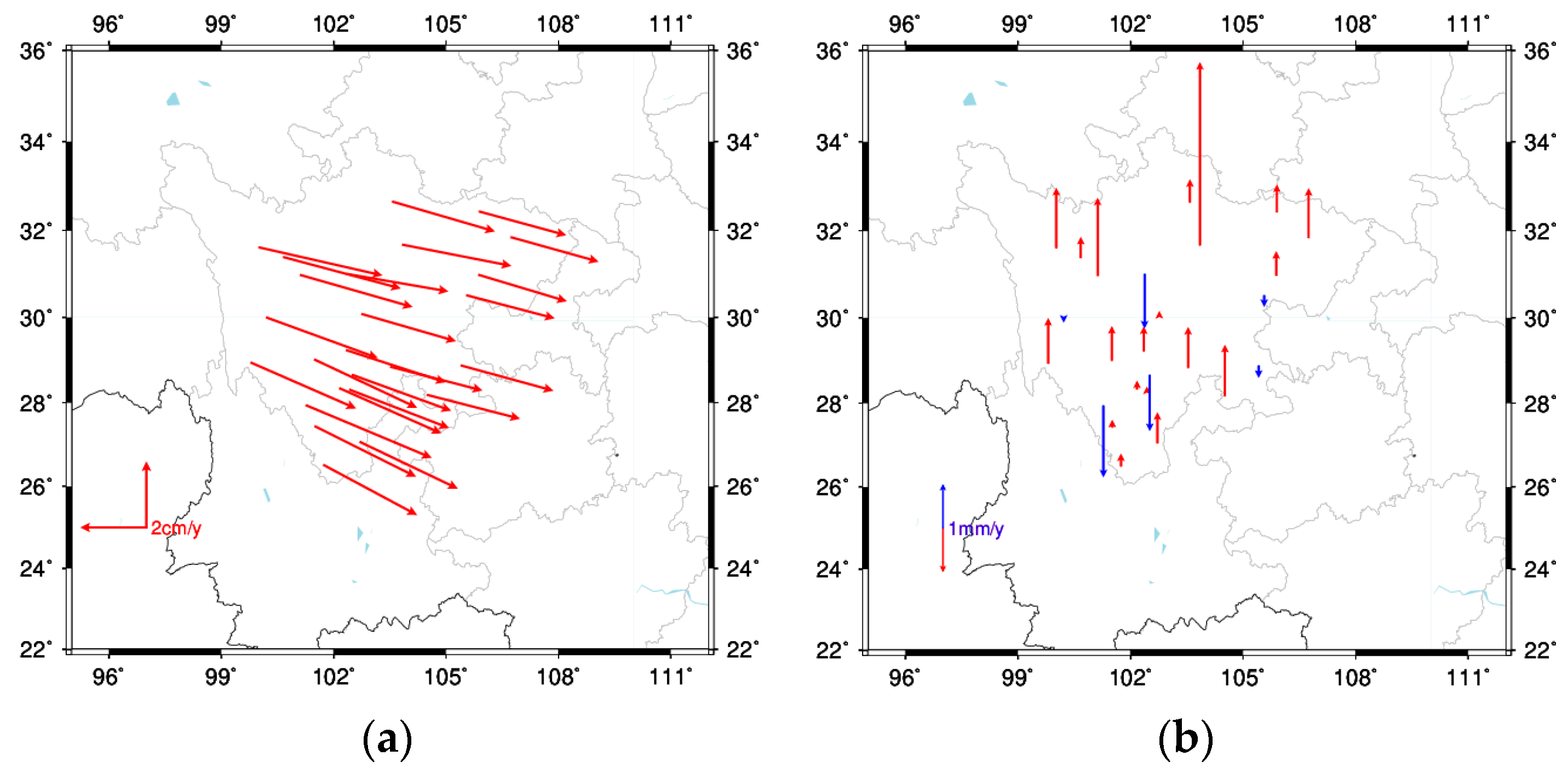
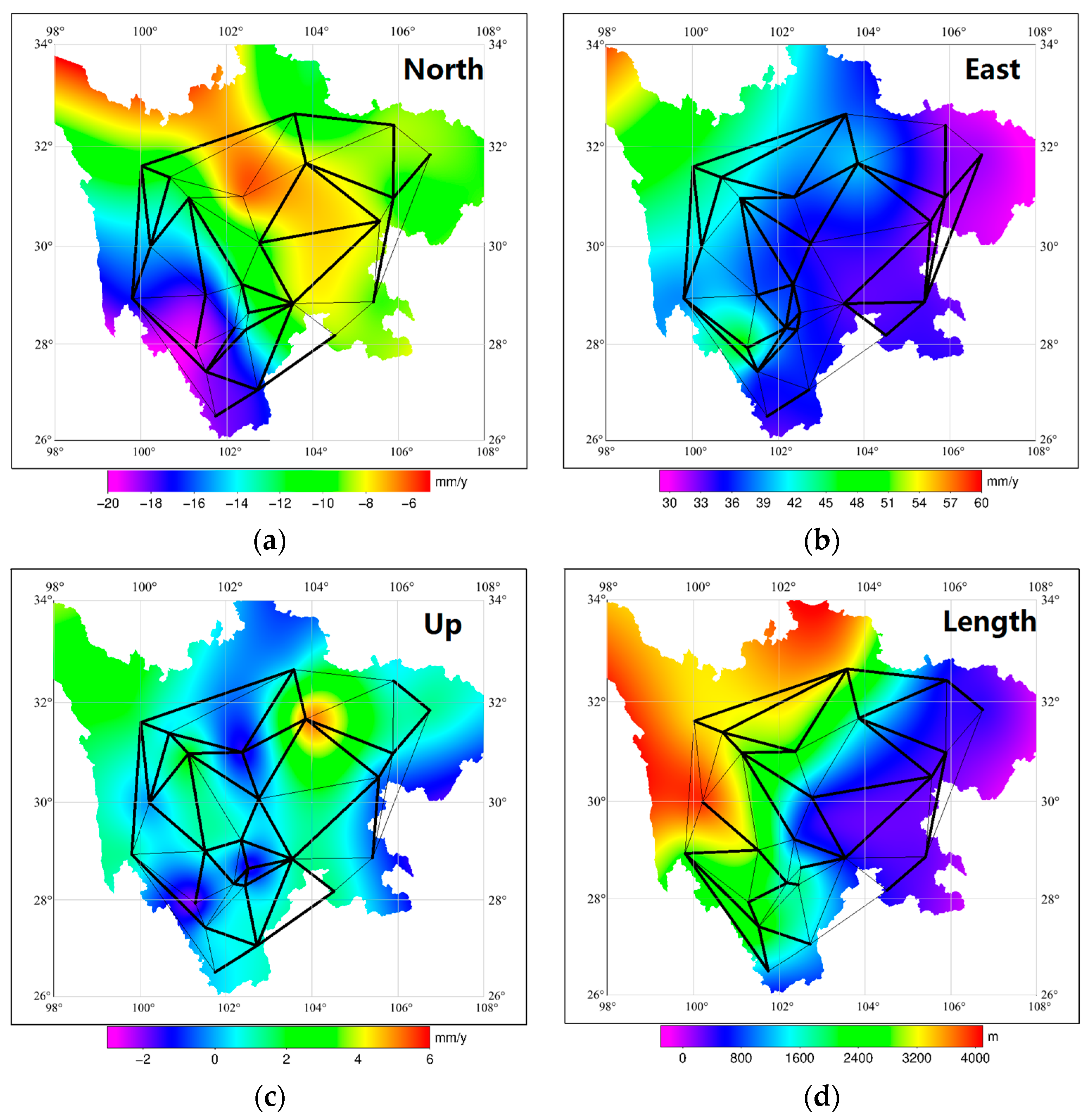
• Analyzing the annual change rate of the north–south component of the baseline, the baseline in the north–east direction is mainly shortened, with a mean annual change rate of −2.7 mm/y, concentrated in the western and northern areas of Sichuan. The bottom graph shows that the movement of the plates in the region is smoother in the north–south direction. Some of the baselines in the north–west direction are in a stretching state, with a mean annual rate of change of 2.0 mm/y, concentrated in the south-central part of Sichuan. The more intense plate motions in the region may be one of the reasons for the baseline stretching.
• The annual rate of change of the east–west component of the baseline is analyzed, and a large number of baselines in the north–east direction are shortening year by year, concentrated in the central and northern areas (68%), with a mean annual rate of change of −3.0 mm/y. The bottom graph shows that the movement of the plates in the region is smoother in the east–west direction, which may have caused the baseline stretching. Some baselines in the north–west and north–east directions are mainly in a stretching trend, with a mean annual rate of change of 2.7 mm/y.
• The annual rate of change of the vertical component of the baseline was analyzed and 68% of the baseline showed a shortening trend characteristic with a mean annual rate of change of −1.4 mm/y. A small number of baselines were in a stretched state with a mean annual rate of change of 1.1 mm/y. As can be seen from the bottom graph, the shortened baselines are mainly concentrated in the subsidence area, indicating that ground subsidence may cause baseline shortening in the Sichuan region.
• From the annual rate of change in the shortening trend baseline, the vertical component is 1.3 mm/y and 1.6 mm/y lower than the north–south and east–west components, respectively. From the annual rate of change in the stretching trend baseline, the vertical component is 0.9 mm/y and 1.6 mm/y lower than the north–south and east–west components, respectively, showing a more stable baseline in the vertical direction.
• Analyzing the annual rate of change of baseline lengths, the baselines in the north–west direction are mainly dominated by a shortening trend, with a mean annual rate of change of −2.8 mm/y, showing that these baselines are shortened on a scale of 2.8 mm per year; some of the baselines in the north–east and north–west directions are dominated by a stretching trend, with a mean annual rate of change of 2.6 mm/y, with more obvious changes. From the bottom graph, it can be seen that the topography of Sichuan gradually declines from northwestern to southeastern, and the baseline of scale shortening is mainly concentrated in the region with relatively smooth topography, while the baseline of the region with larger drop is dominated by stretching, which may provide some new ideas for the study of baseline change.

3.4. Analysis of Random Influence between Reference Stations and Model Construction

The random influence among the reference stations refers to the effect of the motion trend of each reference station in the horizontal and vertical directions on the motion trend of the baseline in the horizontal and vertical directions. The magnitude of the random influence of the reference stations in adjacent areas is mainly determined by finding the standard deviation of each direction of the residual sequence after excluding the baseline CME.

The statistics of the random influence of each direction of the baseline is calculated. The results show that average random influence of the baseline is larger in the north–south and east–west components, 0.39 mm and 0.54 mm, respectively, and smaller in the vertical component and the long component of the baseline, 0.02 mm and 0.22 mm, respectively. The random influence between the reference stations is mainly distributed in the north–south and east–west directions.

The random influence model treats the random influence as a random variable and fits its covariance function. The covariance function is fitted to visualize the spatial distribution characteristics of the random influence. The random influence of each directional component of the baseline was fitted by baseline length statistics using four different functional models (Figure 8).

The Hirvonen function model fits poorly, especially in the L direction, and the Gaussian, polynomial and exponential function models fit more closely to the random influence values with smooth fitting curves.

Table 4. Error statistics of fitting points (unit: mm).

Statistics		Gauss	Hirvonen	Polynomial	Exponential
N	MAX	3.58	3.14	2.03	2.17
	MIN	0.28	0.27	0.57	0.10
	AVE	1.78	1.52	1.22	1.20
	RMS	2.08	1.76	1.34	1.41
E	MAX	4.21	3.14	1.47	3.09
	MIN	0.24	0.65	0.16	0.37
	AVE	2.12	1.72	0.66	1.33
	RMS	2.42	1.95	0.83	1.66
U	MAX	0.44	0.51	0.25	0.38
	MIN	0.01	0.08	0.04	0.04
	AVE	0.16	0.26	0.13	0.17
	RMS	0.25	0.30	0.16	0.21
L	MAX	3.98	10.85	2.12	4.03
	MIN	0.14	0.88	0.68	0.02
	AVE	1.53	5.02	1.38	2.40
	RMS	2.07	6.10	1.49	2.76

demonstrates the fitted point errors. The polynomial fit has the smallest error in fitting all baseline components, and the fitting effect of each component is improved by 5%, 50%, 23.8% and 46%, respectively, compared with the exponential function fit. The improvement is most obvious in the E direction, and it is better than the exponential function fit and the Hirvonen function fit. Therefore, using a polynomial function as a random influence covariance function fitting method can effectively improve the fitting accuracy.

4. Discussion

The spatiotemporal relative motion of the Sichuan regional reference station is influenced by the external environment, geological factors and other non-tectonic signals. The horizontal motion of the reference station is mainly concentrated in the southeast direction and the motion trend in the vertical direction is mainly uplift. The baseline components show mainly north–south compression and east–west stretching, which are consistent with the direction of crustal deformation in the Sichuan region, suggesting that the collision and wedging of the Indian plate with the Eurasian plate is still the main source of tectonic motion in mainland China [28].

Differences in processing software and strategies, noise models or details of the sites defining the reference system can affect the uncertainty of the velocity field [10]. The most advanced version was not used in the solution strategy of this study, such as the old one (IERS03) used for the solid tide correction model. ITRF2020 is the latest enhanced terrestrial reference frame that applies motion constraints to the complete time series of the four techniques with more reliable origin positions and accuracy over time [29]. We used ITRF2014 from 2015 to 2021 instead of the latest ITRF2020, which may also have a slight influence on the accuracy of the velocity field. Also, considering the complexity of the topography in the Sichuan region, the GNSS time series of the stations in the region inevitably contain a residual signal, which should be modeled deterministically or stochastically for improving the accuracy of the GNSS time series [30]. In addition, the lower time span (seven years) makes it possible for random noise to affect the amount of vertical coordinate change, making it unreliable to describe and compare velocities at each site in detail. Therefore, this study reflects the uplift in Sichuan region through the overall change. Seasonal variations, load model errors and component shares of thermoelastic variability in horizontal and vertical deformations have been explained [31]. If a cleaner time series is desired, noise models need to be considered in addition to filtered CME [15]. In the future, the rationality of using the PCA method can also be investigated by comparing the percentage of components with the corresponding seasonal variations and load model errors [11,14].

In terms of modeling variance-covariance functions with random influence, the Gauss, Hirvonen and exponential functions mentioned in Section 2.4 are positively definite, and thus the parameter k in the function model does not affect the model’s positive definiteness to some degree. However, polynomial functions do not have positive definiteness, so it is important to determine the acceptable range of variation of the parameter k. Therefore, we focus on the acceptable range of variation of the parameter k in polynomial functions.

The function models fitted in the paper are generally predicated on small regional scales, so baseline lengths of up to 300 km are generally chosen. Taking the N direction as an example, the coefficients k1, k2 and k3 of the model of the function fitted by the cubic polynomial are −8.6 × 10⁻⁴, −2.0 × 10⁻⁶ and 5.4 × 10⁻⁹, respectively. In order to maintain the positive definiteness of the function model, three schemes are used to test the Sichuan region, mainly discussing the range of values of the parameter k. Figure 9 shows the results of the tests.

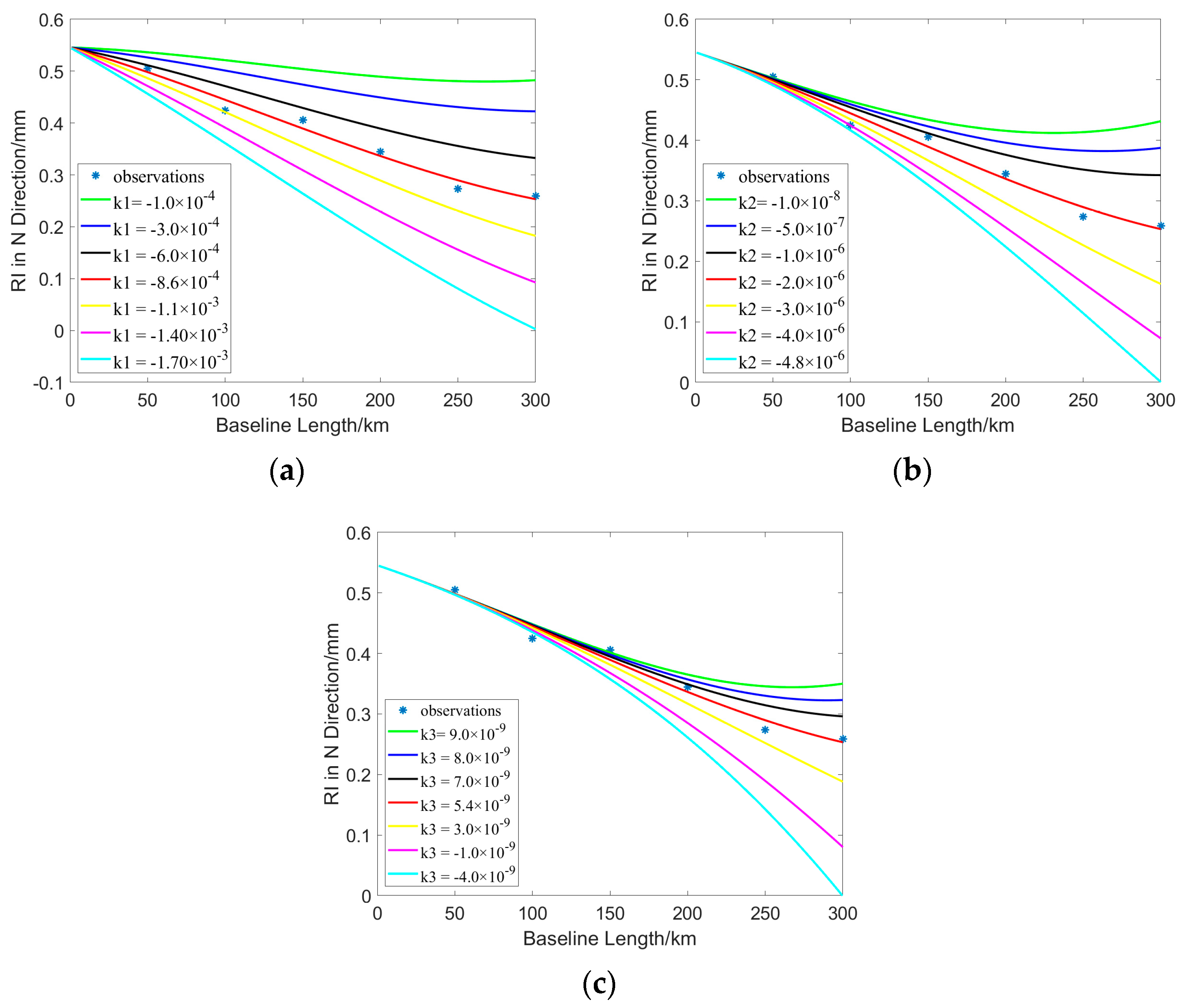
• Set k2 and k3 to the constants that have been calculated and adjust the value of k1;
• Set k1 and k3 to the constants that have been calculated and adjust the value of k2;
• Set k1 and k2 to the constants that have been calculated and adjust the value of k3.

The following results can be drawn from Figure 9:

• Since k1, k2 and k3 are all variables, it is not possible to determine the range of values of all three variables at the same time. Therefore, the control variable method is used to analyze the effect of a particular variable on the positive definiteness of the function;
• In all three schemes, the polynomial fit value decreases as the value of the single variable k decreases. In particular, at values of −1.70 × 10⁻³ for k1, −4.8 × 10⁻⁶ for k2 and −4.0 × 10⁻⁹ for k3, the function fit value is close to zero. In order to maintain the positive definiteness of the function, the single variable k may not be smaller than the above values, respectively;
• The polynomial function model does not have positive definiteness, so the k value needs to be carefully chosen to fulfill the requirement. Meanwhile, the method for calculating the range of k-values of the function model in the E, U and L components is also similar to that of the N component, which will not be discussed here.

5. Conclusions

This study analyzes the time series of reference stations and baselines in the Sichuan region by the LSP method. The CME is eliminated for the coordinate series and the velocity field of the Sichuan region is constructed to investigate the spatiotemporal motion direction of the regional frame. A covariance model of the random effects of the baseline components is also constructed to characterize the random effects of the regional reference frame. The Sichuan region is mainly characterized by annual cycles in all directions. The covariance error reaches mm level between the reference station and the baseline, which is highly significant in the vertical direction. The temporal motion of the Sichuan region is mainly dominated by the southeast direction, with an overall uplift in the vertical direction. The polynomial function is more suitable for constructing the fitted random effect covariance model. In the future, exploring the causal mechanisms of nonlinear variations in coordinate time series and their quantitative impact values can be helpful for the study of reference frame’s intrinsic motion patterns and the relative motions between different plates.

References

1. Rebischung, P.; Altamimi, Z.; Ray, J.; Garayt, B. The IGS contribution to ITRF2014. J. Geod. 2016, 90, 611–630. [Google Scholar] [CrossRef]
2. Altamimi, Z.; Rebischung, P.; Métivier, L.; Collilieux, X. ITRF2014: A new release of the International Terrestrial Reference Frame modeling nonlinear station motions. J. Geophys. Res. Solid Earth 2016, 121, 6109–6131. [Google Scholar] [CrossRef]
3. Bao, Y.; Yu, X.; Wang, G.Q.; Zhou, H.J.; Ding, X.G.; Xiao, G.R.; Shen, S.L.; Zhao, R.B.; Gan, W.J. SChina20: A stable geodetic reference frame for ground movement and structural deformation monitoring in South China. J. Surv. Eng. 2021, 147, 04021006. [Google Scholar] [CrossRef]
4. Peng, Y.; Dong, D.N.; Chen, W.; Zhang, C.L. Stable regional reference frame for reclaimed land subsidence study in East China. Remote Sens. 2022, 14, 3984. [Google Scholar] [CrossRef]
5. Rizos, C. Alternatives to current GPS-RTK services and some implications for CORS infrastructure and operations. GPS Solut. 2007, 11, 151–158. [Google Scholar] [CrossRef]
6. Wang, G.Q.; Bao, Y.; Gan, W.J.; Geng, J.H.; Xiao, G.R.; Shen, J.S. NChina16: A stable geodetic reference frame for geological hazard studies in North China. J. Geodyn. 2018, 115, 10–22. [Google Scholar] [CrossRef]
7. Yu, J.; Wang, G. Introduction to the GNSS geodetic infrastructure in the Gulf of Mexico Region. Surv. Rev. 2017, 49, 51–65. [Google Scholar] [CrossRef]
8. Kenyeres, A.; Bellet, J.G.; Bruyninx, C.; Caporali, A.; Doncker, F.; Droscak, B.; Duret, A.; Franke, P.; Georgiev, I.; Bingley, R.; et al. Regional integration of long-term national dense GNSS network solutions. GPS Solut. 2019, 23, 122. [Google Scholar] [CrossRef]
9. Fazilova, D.; Ehgamberdiev, S.; Kuzin, S. Application of time series modeling to a national reference frame realization. Geod. Geodyn. 2018, 9, 281–287. [Google Scholar] [CrossRef]
10. García-Armenteros, J.A. Topo-Iberia CGPS network: A new 3D crustal velocity field in the Iberian Peninsula and Morocco based on 11 years (2008–2019). GPS Solut. 2023, 27, 155. [Google Scholar] [CrossRef]
11. Zhou, W.; Ding, K.H.; Liu, P.; Lan, G.H.; Ming, Z.T. Spatiotemporal filtering for continuous GPS coordinate time series in mainland China by using independent component analysis. Remote Sens. 2022, 14, 2904. [Google Scholar] [CrossRef]
12. Yu, J.S.; Tan, K.; Zhang, C.H.; Zhao, B.; Wang, D.Z.; Li, Q. Present-day crustal movement of the Chinese mainland based on Global Navigation Satellite System data from 1998 to 2018. Adv. Space Res. 2019, 63, 840–856. [Google Scholar] [CrossRef]
13. Yue, C.Y.; Dang, Y.M.; Dai, H.Y.; Yang, Q.; Wang, X.K. Crustal deformation characteristics of Sichuan-Yunnan region in China on the constraint of multi-periods of GPS velocity fields. Adv. Space Res. 2018, 61, 2180–2189. [Google Scholar] [CrossRef]
14. Zhou, M.S.; Guo, J.Y.; Liu, X.; Shen, Y.; Zhao, C.M. Crustal movement derived by GNSS technique considering common mode error with MSSA. Adv. Space Res. 2020, 66, 1819–1828. [Google Scholar] [CrossRef]
15. Niu, Y.J.; Rebischung, P.; Li, M.; Wei, N.; Shi, C.; Altamimi, Z. Temporal spectrum of spatial correlations between GNSS station position time series. J. Geod. 2023, 97, 12. [Google Scholar] [CrossRef]
16. Hu, S.Q.; Chen, K.J.; Zhu, H.; Wang, T.; Zhao, Q.; Yang, Z.Y. Potential Contributors to CME and Optimal Noise Model Analysis in the Chinese Region Based on Different HYDL Models. Remote Sens. 2023, 15, 945. [Google Scholar] [CrossRef]
17. Ma, X.J.; Liu, B.; Dai, W.J.; Kuang, C.L.; Xing, X.M. Potential Contributors to Common Mode Error in Array GPS Displacement Fields in Taiwan Island. Remote Sens. 2021, 13, 4221. [Google Scholar] [CrossRef]
18. Li, W.H.; Li, F.; Zhang, S.K.; Lei, J.T.; Zhang, Q.C.; Yuan, L.X. Spatiotemporal filtering and noise analysis for regional GNSS network in Antarctica using independent component analysis. Remote Sens. 2019, 11, 386. [Google Scholar] [CrossRef]
19. Bian, Y.K.; Yue, J.P.; Ferreira, V.G.; Cong, K.L.; Cai, D.J. Common mode component and its potential effect on GPS-inferred crustal deformations in Greenland. Pure Appl. Geophys. 2021, 178, 1805–1823. [Google Scholar] [CrossRef]
20. Wdowinski, S.; Bock, Y.; Zhang, J.; Fang, P.; Genrich, J. Southern California permanent GPS geodetic array: Spatial filtering of daily positions for estimating coseismic and postseismic displacements induced by the 1992 Landers earthquake. J. Geophys. Res. Solid Earth 1997, 102, 18057–18070. [Google Scholar] [CrossRef]
21. Bian, Y.K.; Li, Z.; Huang, Z.Q.; He, B.; Shi, L.L.; Miao, S. Combined GRACE and GPS to Analyze the Seasonal Variation of Surface Vertical Deformation in Greenland and Its Influence. Remote Sens. 2023, 15, 511. [Google Scholar] [CrossRef]
22. Pan, Y.J.; Chen, R.Z.; Ding, H.; Xu, X.Y.; Zheng, G.; Shen, W.B.; Xiao, Y.X.; Li, S.Y. Common mode component and its potential effect on GPS-inferred three-dimensional crustal deformations in the Eastern Tibetan Plateau. Remote Sens. 2019, 11, 1975. [Google Scholar] [CrossRef]
23. Lomb, N.R. Least-squares frequency analysis of unequally spaced data. Astrophys. Space Sci. 1976, 39, 447–462. [Google Scholar] [CrossRef]
24. VanderPlas, J.T. Understanding the lomb–scargle periodogram. Astrophys. J. Suppl. Ser. 2018, 236, 16. [Google Scholar] [CrossRef]
25. Yu, H.J.; Chen, Q.J.; Sun, Y.; Sosnica, K. Geophysical Signal Detection in the Earth’s Oblateness Variation and Its Climate-Driven Source Analysis. Remote Sens. 2021, 13, 2004. [Google Scholar] [CrossRef]
26. Garate, J.; Martin-Davila, J.; Khazaradze, G.; Echeverria, A.; Asensio, E.; Gil, A.J.; Lacy, M.C.; Armenteros, J.A.; Ruiz, A.M.; Gallastegui, J.; et al. Topo-Iberia project: CGPS crustal velocity field in the Iberian Peninsula and Morocco. GPS Solut. 2015, 19, 287–295. [Google Scholar] [CrossRef]
27. He, X.X.; Hua, X.H.; Yu, K.G.; Xuan, W.; Lu, T.D.; Zhang, W.; Chen, X. Accuracy enhancement of GPS time series using principal component analysis and block spatial filtering. Adv. Space Res. 2015, 55, 1316–1327. [Google Scholar] [CrossRef]
28. Wu, J.C.; Song, X.Y.; Wu, W.W.; Meng, G.J.; Ren, Y.Y. Analysis of crustal movement and deformation in mainland China based on CMONOC baseline time series. Remote Sens. 2021, 13, 2481. [Google Scholar] [CrossRef]
29. Altamimi, Z.; Rebischung, P.; Collilieux, X.; Métivier, L.; Chanard, K. ITRF2020: An augmented reference frame refining the modeling of nonlinear station motions. J. Geod. 2023, 97, 47. [Google Scholar] [CrossRef]
30. Reguzzoni, M.; Rossi, L.; De Gaetani, C.I.; Caldera, S.; Barzaghi, R. GNSS-based dam monitoring: The application of a statistical approach for time series analysis to a case study. Appl. Sci. 2022, 12, 9981. [Google Scholar] [CrossRef]
31. Niu, Y.J.; Wei, N.; Li, M.; Rebischung, P.; Shi, C.; Chen, G. Quantifying discrepancies in the three-dimensional seasonal variations between IGS station positions and load models. J. Geod. 2022, 96, 31. [Google Scholar] [CrossRef]
Figure 1. Distribution of the IGS and Sichuan CORS(SCCORS) stations. (a) Triangulation network of regional reference stations in Sichuan. (b) Distribution of the 12 IGS stations.
Applsci 14 00432 g001
Figure 2. Flow chart of the analysis of the spatiotemporal characteristics of reference frame.
Applsci 14 00432 g002
Figure 3. Results of the Lomb–Scargle periodogram method for analyzing the time-frequency transformation of time series. (a,b) represent the spectral analysis results of the reference stations SCMN and SCXC, respectively. (c,d) represent the spectral analysis results of baseline SCML-SCMN and SCJL-SCXC, respectively.
Applsci 14 00432 g003
Figure 4. Comparison of residual SCMN series before and after removing CME. (a) Residual sequence of SCMN without removing CME; (b) CME extracted from SCMN; (c) Residual sequence of SCMN after removing CME.
Applsci 14 00432 g004
Figure 5. Comparison of residual SCML-SCMN baseline series before and after removing CME. (a) Residual sequence of SCML-SCMN without removing CME; (b) CME extracted from SCML-SCMN; (c) Residual sequence of SCML-SCMN after removing CME.
Applsci 14 00432 g005
Figure 6. Movement rate of the Sichuan regional reference stations in the (a) horizontal direction and (b) vertical direction.
Applsci 14 00432 g006
Figure 7. Distribution of annual change rate of Sichuan regional baseline in (a) N Component; (b) E Component; (c) U Component; (d) L Component, respectively. The bolded baseline indicates that the annual rate of change of the baseline is negative, showing a shortening trend; the unbolded baseline has a positive annual rate of change, showing an extension trend.
Applsci 14 00432 g007
Figure 8. Function Model fitting of Residual Baseline Series in (a) N Component; (b) E Component; (c) U Component; (d) L Component. RI on the vertical axis represents random influence.
Applsci 14 00432 g008
Figure 9. Effect of parameter k on the fitting of the functional model under different schemes, (ac) only adjusts the values of k1, k2 and k3 respectively.
Applsci 14 00432 g009