Abstract
A variety of structural members and non-structural components, including bridge piers, museum artifacts, furniture, or electrical and mechanical equipment, can uplift and rock under ground motion excitations. Given the inherently non-linear nature of rocking behavior, employing machine learning algorithms to predict rocking response presents a notable challenge. In the present study, the performance of supervised ML algorithms in predicting the maximum seismic response of free-standing rigid blocks subjected to ground motion excitations is evaluated. As such, both regression and classification algorithms were developed and tested, aiming to model the finite rocking response and rocking overturn. From this point of view, it is essential to estimate the maximum rocking rotation and to efficiently classify its magnitude by successfully assigning respective labels. To this end, a dataset containing the response data of 1100 rigid blocks subjected to 15,000 ground motion excitations, was employed. The results showed high accuracy in both the classification ( accuracy) and regression (coefficient of determination ) tasks.
1. Introduction
In light of field observations conducted in the aftermath of the 1960 Chile earthquakes, a prevailing consensus has emerged, underscoring that the uplifting and rocking of structures on their foundations during severe ground motions leads to an enhancement of seismic performance [1]. In contrast to fixed-base structural systems, whose seismic response is primarily governed by the dissipative energy process occurring at predefined locations through damage, free-standing structures’ rocking response results in diminished structural damage, owing to the presence of negative post-uplift stiffness [2]. Apart from large-scale structures [3,4,5,6,7,8,9,10,11,12,13], non-structural elements within buildings may also uplift and rock [14,15,16] in response to floor accelerations [17,18].
The pioneering work of Housner [1] highlighted the key features of rocking block dynamics. In particular, the initiation of the rocking effect under earthquake loading necessitates a minimum threshold of acceleration, the value of which is contingent upon the system’s geometry. After uplift, the system exhibits negative stiffness, attributable to its self-weight acting as a restoring force. Due to the negative stiffness, the vibration period of a rocking oscillator is not constant but continually varies, depending on its rotation, while the stability of rocking bodies is governed by scale-size effects. With the recognition of the beneficial effects of rocking response on the seismic performance of structures, a plethora of researchers have studied the phenomenon [19,20,21,22].
It is imperative to ensure that the system will remain stable and not undergo overturning during its dynamic response in order to harness the advantages of the rocking effect. From this point of view, estimating the maximum rocking response is essential. Nonetheless, achieving this objective is not a straightforward endeavor, primarily attributable to the pronounced non-linearity inherent in the motion, which arises from the negative stiffness characteristic of the rocking oscillator [2]. It is apparent that even minor alterations in the parameters of the rocking oscillator or in the attributes of the ground motion record yield entirely distinct responses [23]. Hence, the seismic response of rocking systems should be assessed within a probabilistic framework [24,25,26,27,28,29,30,31]. To this end, it is necessary to perform a vast number of non-linear time history analyses to assess the probabilistic distribution of seismic demands.
It is evident that non-linear time history analysis of structures is a time-consuming process that also requires high computational resources. To overcome this bottleneck, a substantial research effort in the field of soft computing methods for the rapid evaluation of the seismic response of structures has been undertaken over the past two decades. The majority of machine learning (ML) applications in this field primarily focus on predicting seismic demands for various types of structures, including reinforced concrete [32,33,34], steel [35,36,37], and timber [38] buildings, as well as bridges [39]. For bridges, in particular, methods such as convolutional neural networks (CNNs), in conjunction with signal processing, have been implemented for early damage detection and warning [40]. In addition to capturing the precise values of engineering demand parameters (EDPs), the capability of machine learning methods to classify seismic responses into levels corresponding to different damage limit states has been investigated [41,42,43]. Given that assessing the seismic performance of structures in terms of fragility is the basis of performance-based earthquake engineering, numerous applications of ML methods in seismic fragility and risk have also been presented in the literature [44,45,46].
Although there is a plethora of ML implementations on fixed-based or seismically isolated structures, there is a lack of implementations on rocking structures. To the best of the authors’ knowledge, there are only four studies that utilize ML algorithms to predict the response of rocking oscillators. Specifically, Gerolymos et al. [47] developed an ANN to predict the overturning response of rigid blocks under pulses, while Pan et al. [48] proposed an ANN with adaptive training to predict the time-history response of a rocking block. Moreover, Achmet et al. [49] implemented ML algorithms to predict whether or not a given rocking block will overturn under pulse excitations and natural ground motions. Recently, Shen and Málaga-Chuquitaype [50] presented a physics-informed convolutional NN for the simulation of the rocking motion of rigid blocks.
The present study aims to evaluate data-driven methods for the estimation of the seismic demands, in terms of rocking rotations, of free-standing rigid blocks under seismic excitations. To this end, 1100 rigid blocks subjected to 15,000 ground motions were analyzed, and a dataset of 16,500,000 responses was generated, covering a wide range of free-standing structures. Since rocking oscillators may overturn during the response, classification ML algorithms are evaluated to predict structural collapse. In cases where the rocking oscillator presents a stable response, regression ML algorithms are utilized to predict the maximum rocking rotation.
The novelty of the present study compared to the publications mentioned above is threefold. Firstly, the modeling is not limited to whether or not overturning occurs, as in [49], but a regression model was also built to estimate the maximum rotation angle in cases where overturning does not occur. Moreover, unlike Pan et al. [48], this maximum rotation angle is estimated directly, instead of computing the whole time-history response of the rocking block. Finally, a larger dataset with a richer set of features is employed, allowing the models to learn more complex patterns in the data.
Our paper is organized as follows. In Section 2.1 and Section 2.2, the basic theory of the rocking block problem is described, as well as the features that comprise our dataset. In Section 3, the ML algorithms that are employed for the classification and regression are presented. Finally, in Section 4, the main results of our methodology are discussed, using well-known classification and regression metrics.
2. Materials and Methods
2.1. Dynamics of Rigid Rocking Blocks
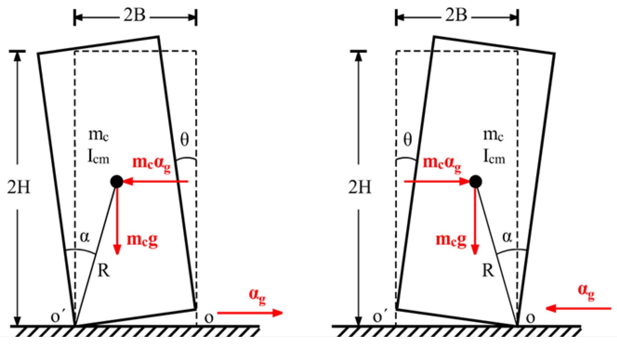
The dynamic response of a free-standing rigid block is considered to be described by a single-degree-of-freedom rocking oscillator. With reference to Figure 1, the system is characterized by the mass , the semi-diagonal length R, the rotational moment of inertia around its center of mass, , and the slenderness, . According to the model’s assumption, no sliding and bouncing phenomena are considered. As such, the dynamic response is adequately described by the tilt angle around the pivot points O and O’. Since the rocking block is assumed to be rigid; the system remains inactive () until the horizontal overturning force, resulting from ground acceleration, surpasses the restoring forces stemming from its own weight. The acceleration required to trigger uplift is expressed as follows:
where the upper (−) and lower (+) signs specify the initiation of rocking around the right () and left () pivot points, respectively, represents the ground acceleration and g is the gravitational acceleration.
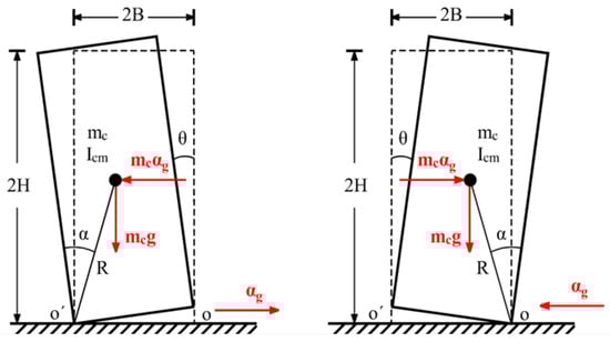
Figure 1.
Uplift of the free-standing rigid block due to ground acceleration.
The rocking response of rectangular free-standing rigid blocks is described by the following equation of motion [21]:
where denotes the signum function, denotes the second derivative with respect to the time of , and p is the frequency parameter of the block, which is defined as follows:
where the last equality stems from the fact that for rectangular blocks. During the response, energy is dissipated only at impact instant when the pivot point changes. The energy loss is expressed by the coefficient of restitution (COR) that defines the ratio between the pre () and post () impact rotational velocities. The COR is given by the following equation [1]:
where and denote the first derivative with respect to the times of and , respectively.
2.2. Dataset Description
In order to evaluate the efficiency of ML algorithms to predict the maximum rocking response of free-standing rigid blocks, 1100 rocking blocks are considered in total. As indicated in Equation (2), it is evident that the frequency parameter p and the slenderness are the structural parameters that affect the rocking response. Therefore, these two parameters are adopted as the input features that characterize the examined blocks. The rocking blocks under examination were created by combining 100 equally spaced values of the frequency parameter (p), which spans from s to 7 s, and 11 equally spaced values of the slenderness parameter (), ranging from to . The adopted range of the frequency parameter corresponds to blocks with semi-diagonals ranging from 0.15 m to 15 m. Thus, the considered database describes the dynamic response of structures ranging from small-sized building contents to rocking bridge piers.
In order to create the data set, the considered blocks are subjected to 5000 natural ground motion acceleration records. Since the slender enough rocking blocks are prone to rocking overturn, the selection of ground motions is based on a minimum peak ground acceleration (PGA) value of 0.05 g to enforce uplift without overturn. Additionally, each record is scaled using three scale factors with values 0.5, 1, and 2. The scaling is performed to derive the full range of possible responses of the examined blocks. The ground motion records set comprises an extensive assortment of seismic data, covering a wide spectrum of seismic events. With [51] values ranging from 100 m/s to 2000 m/s, which correspond to soil classes ranging from A to D, the set accommodates diverse soil conditions. Furthermore, the spans from 0.07 km to 185 km, while the magnitude ranges from 3.2 to 7.9. Moreover, the database encompasses records for all faulting types, offering a comprehensive perspective on seismic activity.
Seismic excitations are highly intricate and necessitate a substantial volume of data for comprehensive characterization. The definition of various ground motion parameters, known as intensity measures (IMs), simplifies the representation of strong ground motions and establishes a connection between seismic hazards and the structural data essential for solving earthquake engineering challenges. Within the realm of earthquake engineering, the most significant features of ground motion encompass amplitude, frequency content, and duration. From this point of view, the 18 IMs listed in Table 1 are considered as input features for the description of the ground motion signal.
In Table 1, are the ground velocity and displacement; are the Fourier amplitudes of the excitation accelerogram and the discrete Fourier transform frequencies, and are the total and “significant” [52] durations of the ground excitation respectively.
For the creation of the dataset, 15,000 time history analyses for each block were conducted, as mentioned above. From the resulting responses, only those where the rocking response was initiated were retained. Also, note that the classification problem of whether or not a rocking response is initiated does not necessitate the use of ML methods since the critical ground acceleration is given by (1). Thus, we obtained 5,782,400 responses in total. From these, in 2,525,847 cases, the excitation resulted in the overturning of the block, while in 3,256,553 it did not. Thus, the class ratio was approximately 56:44, i.e., the dataset did not suffer from the so-called class imbalance problem, which can severely impact the performance of ML algorithms [53,54]. Finally, the maximum seismic rocking rotation was measured, but only for those instances where the block did not overturn.
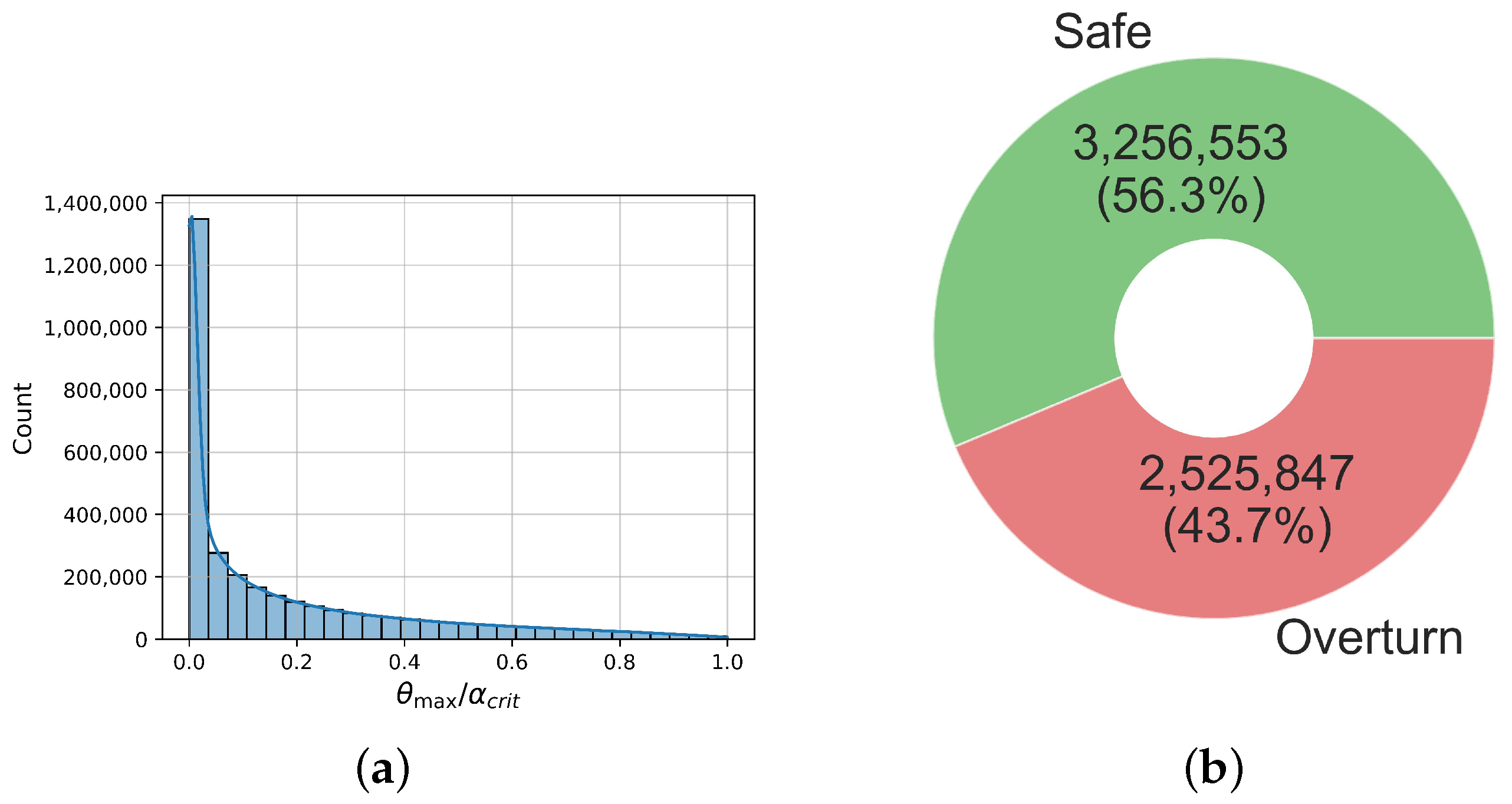
Thus, ultimately, two datasets were obtained, both with 20 features, i.e., the 18 IMs shown in Table 1, as well as the frequency parameter p and slenderness parameter . The first dataset employed in the classification task had 5,782,400 instances, and the target variable was whether the block was overturned or not (safe). The second dataset, which was employed in the regression task, had 3,256,553 instances with the same features, corresponding to those cases in the first dataset where overturning did not occur. In that case, the performance of the examined structural systems is evaluated in terms of the absolute maximum rotation angle normalized to the critical overturning rotation a. As such, this engineering demand parameter (EDP) is considered as target variable in the regression models. Figure 2 summarizes the distribution of these target variables. We can readily observe that most instances had a small maximum rotation, approximately following a gamma distribution.
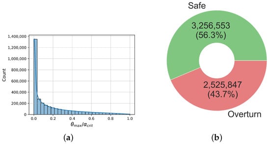
Figure 2.
Visualization of the target variables for the regression and classification sub-problems. (a) Histogram with kernel density estimation for the normalized maximum rotation. (b) Distribution of the “Overturn” variable in our dataset.

Table 1.
Ground motion description input features.
Table 1.
Ground motion description input features.
| Description | References | |
|---|---|---|
| PGA | [55] | |
| PGV | [55] | |
| PGD | [56] | |
| [56] | ||
| - | [57] | |
| - | [25] | |
| [58] | ||
| [58] | ||
| [58] | ||
| [59] | ||
| [28] | ||
| [60] | ||
| [61] | ||
| [62] | ||
| SED | [55] | |
| - | [52] | |
| CAV | [63] | |
| CAD | [63] |
The elevated number of response data enables the training of a reliable model within the considered range of rocking block features. Due to the fact that different rocking structures can be modeled by a rigid block of equivalent frequency parameters and the same slenderness, the trained model can also be used to estimate their maximum response. However, these predictions may be conservative since the database is generated assuming Housner’s coefficient of restitution.
3. Machine Learning Algorithms
As was discussed in Section 2.2, we are dealing with two distinct problems separately and, thus, two independent models to address them have been built. On the one hand, we built a model to predict whether or not the rocking block overturns. In the context of machine learning, this is a binary classification problem. On the other hand, for cases where the block does not overturn, we built a model to estimate the maximum rotation angle, which is a regression problem.
There are many well-established algorithms in the literature of ML for both classification [64] and regression [65]. The large volume of the available dataset calls for adequate computational capacity. We tried numerous ML modeling algorithms in a PC Core i7, using the MATLAB platform version 2020. Moreover, Python (version 3.11.5) programs have also been developed. This paper discusses the architecture and the performance indices values of the most robust ML models that offer high overall accuracy. More specifically, artificial neural networks and regression trees offer strong classification and regression models, respectively, while the gradient boosting modeling approach offers robust models for both tasks. The features used by the models are described in Section 2.2 and Table 1.
3.1. Binary Classification
For the binary classification sub-problem, the following algorithms were considered:
- Artificial neural network (ANN): An artificial neural network consists of a set of nodes (neurons) arranged in layers. The first layer is the input layer, where the input vectors are passed. Subsequently, each neuron takes as input the output of the previous layer and produces a weighted sum of all its inputs, which it then passes through a so-called activation function. This procedure introduces non-linearities, which allow the model to learn complex structures in the data. The final (output) layer for a binary classification problem consists of a single node with a specialized activation function, usually a step function, sigmoid, or , which gives the probability that the given input belongs to the positive class and classifies it according to a user-defined probability threshold. The algorithm learns by minimizing the differences between its predictions and the true values in an iterative process known as backpropagation [66]. The implementation of the ANN classifier was carried out in MATLAB.
- Gradient boosting classifier: The gradient boosting classifier is a meta classifier [67], i.e., it combines weaker models, which are usually decision trees [68]. At each iterative training step, it improves its performance using the current predictions and a user-defined loss function [69]. However, even though this is a powerful algorithm, its training can be very demanding, both in time and computational resources, especially in large datasets with continuous features, such as the one used in the present study. This is because, for the creation of each individual tree, the algorithm must consider each feature and each distinct value separately [70]. To alleviate this, histogram-based methods have been developed [71,72], which partition the numerical values of each continuous feature into bins before training. The implementation was carried out in Python programming language using the dedicated machine learning library scikit-learn [73].
3.2. Regression
For the regression sub-problem, the following algorithms were implemented and compared:
- Regression tree: Regression trees are decision trees in which the target variables can take continuous values instead of class labels in leaves. A decision tree (DT) comprises the following three parts: The nodes (representing the attributes), the branches, and the leaves. The last part is a leaf; the top part is known as the root. Between the root and the leaf, we find the branches. The DT collects and considers the answers to the questions related to the data in order to develop decision rules. This process keeps running and stops when leaves or nodes without branches are found. Testing data are used to determine the generalization potential of the tree. It is important to mention that there is only a single root/a single decision rule from the root towards each leaf [74]. The implementation of this algorithm was carried out in MATLAB.
- Gradient boosting regressor: The algorithm works similarly to the gradient boosting classifier. however, instead of using decision trees, it uses Regression Trees as its base models. Given that it has the same computational limitations as its classification variant, we again opted to use the histogram-based optimized algorithm. The implementation was also carried out using scikit-learn.
- ANN regressor: The algorithm is almost identical to the ANN classifier. The difference is that the activation function of the output layer is usually linear, instead of sigmoid or .
- Random forest regressor: This is an ensemble of Regression Trees. Randomness is introduced to each individual tree by training it on a bootstrapped sample of the original dataset. The final model output is the average of the ensemble.
Finally, we note that, by construction, tree-based algorithms are not susceptible to features with different scales. However, ANN was also employed, which can be susceptible to such scaling. To alleviate this, different scaling techniques can be applied, such as normalization, MinMax scaling or quantile transformer, among others [75]. In the present study, the datasets were preprocessed using a standard MinMax scaler, thus normalizing all the features in the range [0, 1].
3.3. Hyperparameter Optimization
The algorithms mentioned above have a set of so-called hyperparameters that are predefined by the user before training begins. For example, this can include the maximum number of trees in Gradient Boosting, the maximum depth of the decision tree, or the number of hidden layers and neurons per layer in ANN. These hyperparameters can affect the performance of the model and reduce overfitting and, thus, dedicated methodologies have been proposed by researchers to identify the optimal hyperparameter configuration [76]. However, due to the very large size of our dataset and the constraints this imposed, both on time and computational resources, the calibration of the models was carried out using a trial-and-error approach. Table 2 summarizes the hyperparameters that were used for each algorithm. ReLU (rectified linear unit) is defined as
Table 2.
Hyperparameter configuration of the ML models.
Moreover, is the well-known hyperbolic tangent function, defined as
Finally, in Table 3, brief descriptions of these hyperparameters are given.
Table 3.
Hyperparameter descriptions.
4. Results
To train our classification and regression models, a so-called 70-15-15 split was employed. Thus, of our dataset was used for training, from which the algorithm learned the patterns in the data. Another was used as a holdout validation set, which measures the evolution of the performance during training and instructs the algorithm to stop if this deteriorates. Finally, of the data, which the algorithm had not used before, neither for training nor validation, were used as a test set to measure its performance on truly unseen data. In Section 4.1, the results for the classification algorithms are presented, while Section 4.2 presents the results of the regression.
4.1. Classification Results
In order to measure the performance of our classification models, some well-known classification metrics were computed, specifically [77]
where in the above , and are the number of true positive, false positive, false negative, and true negative instances, respectively. In addition to the above, we computed the so-called logistic loss (log-loss), also called binary cross-entropy, which is defined as
where in the above N is the number of vectors in the dataset, are the model’s predictions, which correspond to the probability that a given vector belongs to the positive class and are the actual class labels. Finally, we computed the so-called area under the curve (AUC), which quantifies the balance between the false positive and true positive rates of the model [77]. Table 4 summarizes the above metrics for the two examined classifiers.
Table 4.
Classification metrics on the test dataset of the binary classifiers.
The best-performing classifier, gradient boosting, achieved an overall accuracy of . This fact indicates the overall success of the algorithm to accurately assess the safety of the rigid rocking block under seismic excitation. In addition, the classification metrics are approximately equal for both classes, enhancing the reliability of the predictions.
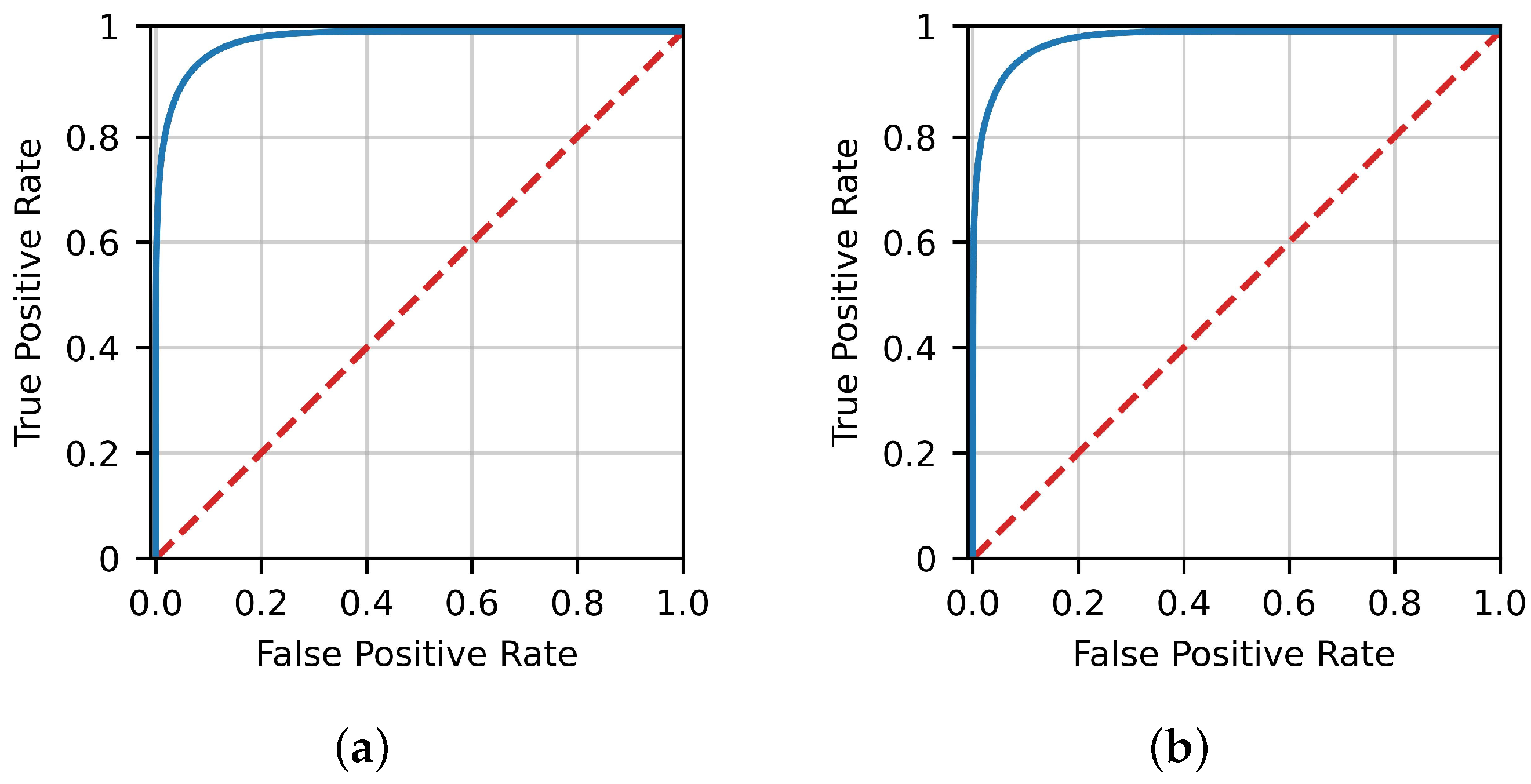
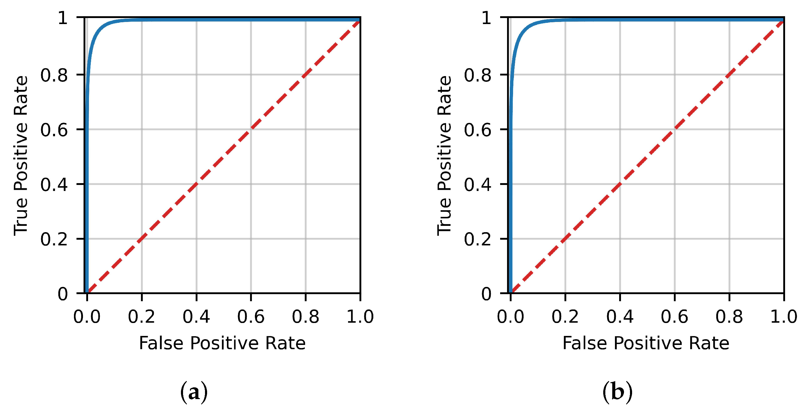
Figure 3 presents the FP-TP rate curves (ROC curves) for ANN, while Figure 4 presents the corresponding curves for Gradient Boosting. It can be readily observed that a very high true positive rate can be achieved without a corresponding large false positive rate.
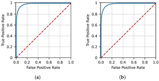
Figure 3.
ROC curves for the train and test dataset of ANN. (a) ANN training ROC. (b) ANN test ROC.
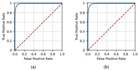
Figure 4.
ROC curves for the train and test dataset of Gradient Boosting. (a) Gradient boosting training ROC. (b) Gradient boosting test ROC.
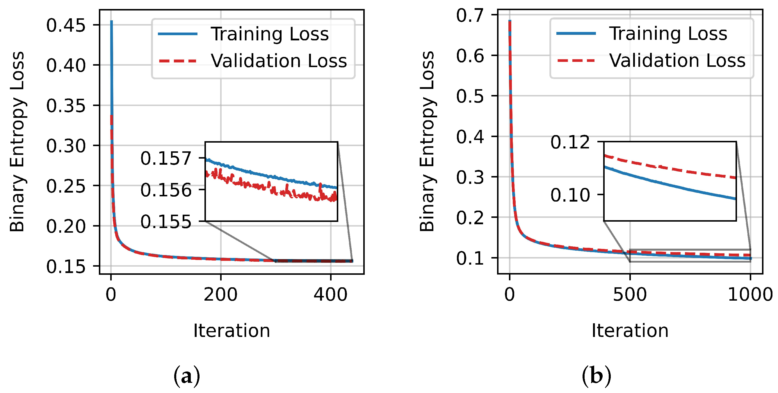
Subsequently, Figure 5 shows the evolution of the training loss of the two examined classifiers. The training stops either when the maximum number of iterations is reached, or when the gain in the validation loss, i.e., the loss measured on a holdout subset of the training set, becomes too small compared to the gain in training loss, i.e., when there is the risk of overfitting. Overfitting would manifest with a significant gap between the training and validation loss curves (generalization gap). However, as can be readily observed, the two curves are very close in our case, so no overfitting has occurred. Finally, Figure 6 shows the corresponding confusion matrices [77] for the train and test set for both classifiers.
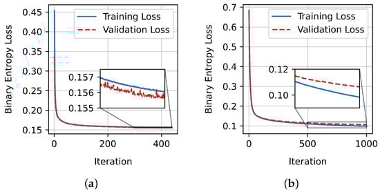
Figure 5.
Training loss curve of the two examined classifiers. (a) Training loss curve of ANN. (b) Training loss curve of gradient boosting.
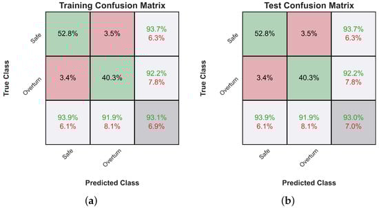

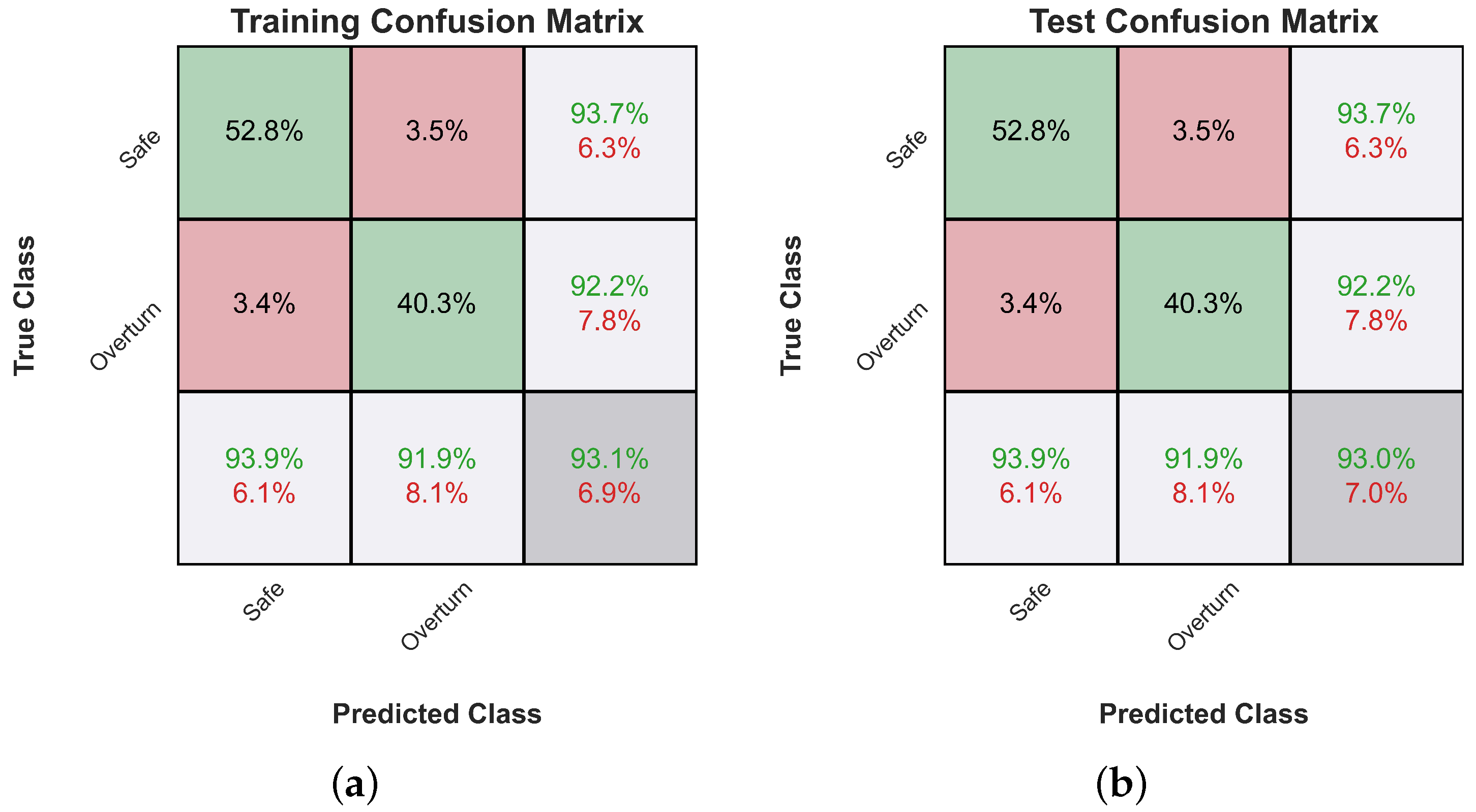
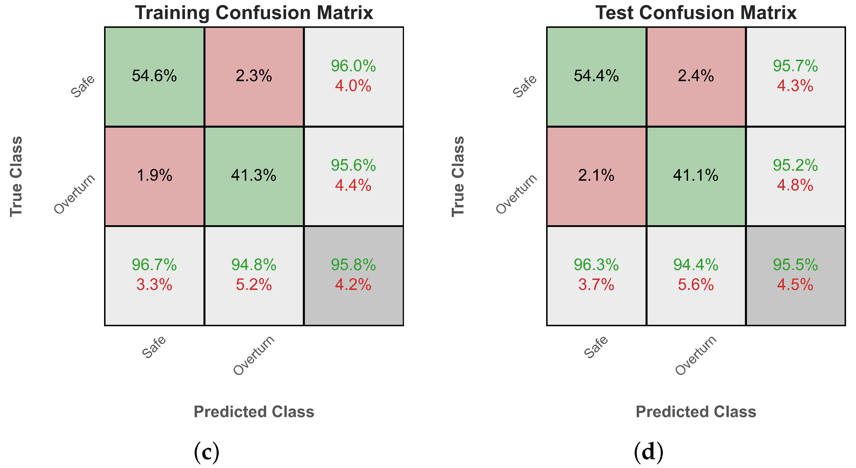
Figure 6.
Confusion matrices for the train and test dataset of the two examined classifiers. (a) ANN training confusion matrix. (b) ANN test confusion matrix. (c) Gradient boosting training confusion matrix. (d) Gradient boosting test confusion matrix.
4.2. Regression Results
Similarly, to measure the performance of our regression models, the well-known metrics of root mean squared error (RMSE), mean absolute error (MAE), and coefficient of determination are employed. Table 5 summarizes the employed regression metrics and their corresponding formulas, while Table 6 summarizes their computed values on the test set for both regression models examined here.
Table 5.
Summary of the employed regression metrics. In the below, and are the true values and model predictions, respectively, and N is the number of samples in the dataset.
Table 6.
Regression metrics on the test dataset of employed models.
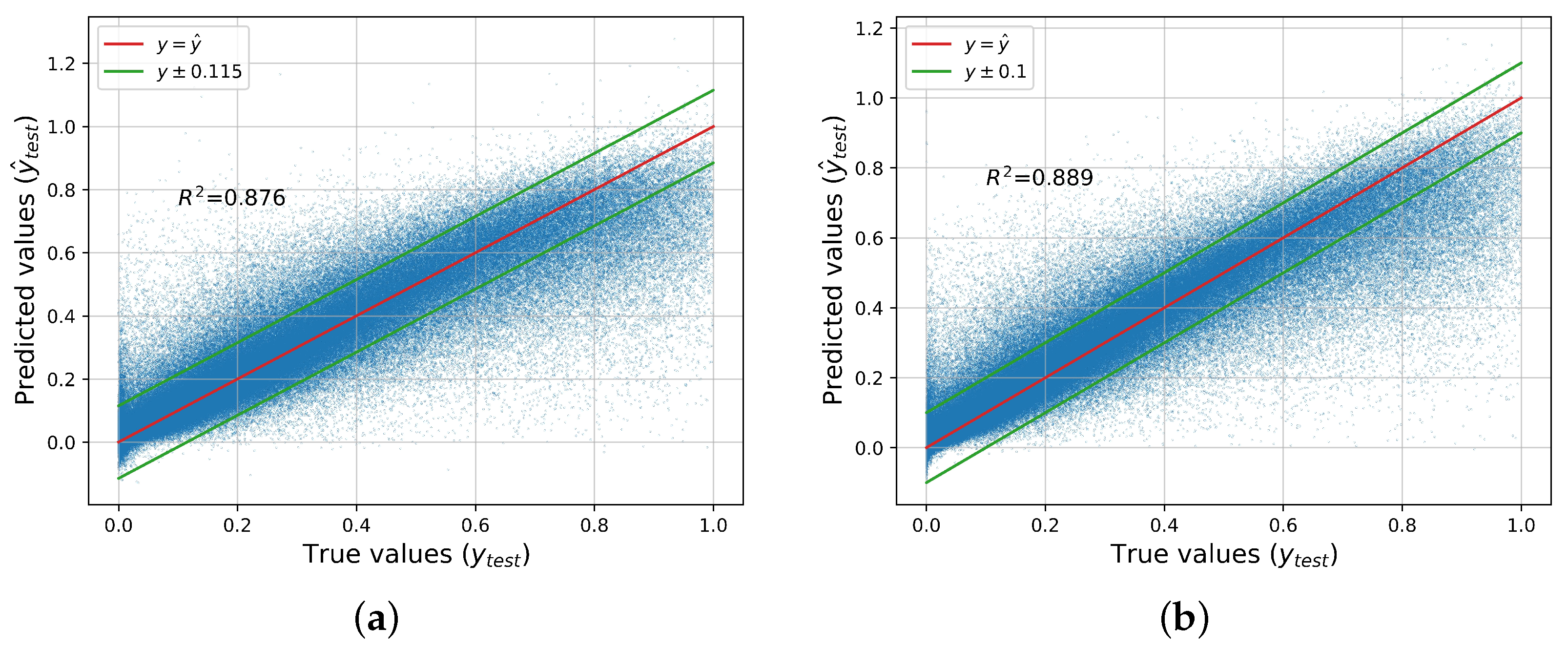
We can readily observe that the gradient boosting regressor outperforms the regression tree, although not by a huge margin. Low MAE, MSE, or RMSE values show that the regression model has high accuracy, which is desired. On the other hand, indicates how well the considered independent variables explain the variability of the dependent parameter. RMSE is a more robust index, indicating how well the model will fit with unseen data (generalization). The RMSE is almost double the MAE for both models, due to the presence of a few very large values in the models’ errors. In Figure 7, the predictions of the two best-performing models, gradient boosting and ANN, versus the actual values of the test dataset, are presented. We also present the thresholds for which we find that approximately or more of the model’s predictions lie within this distance from the true value.
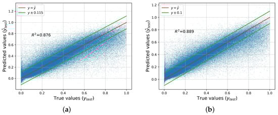
Figure 7.
True values vs. predictions made by the best-performing regressors. (a) ANN. (b) Gradient boosting.
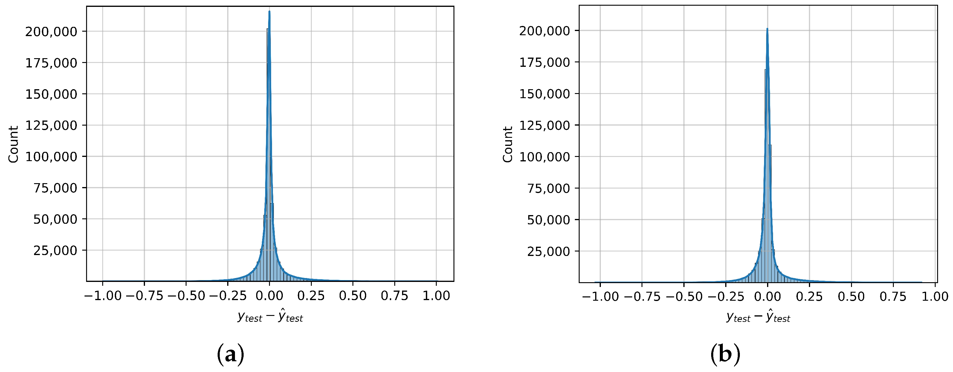
In Figure 8, we present the distribution of the errors in the models’ predictions on the test dataset, along with its kernel density estimation. The errors are not normally distributed, as their distribution is leptokurtic, with , where 3 is the kurtosis of the normal distribution. This fact also means that the distribution has fatter tails and some extreme values exist. However, as was previously mentioned, more than of the errors of the best-performing regressor are in the interval . Furthermore, it can be observed that the errors appear to be symmetrically distributed around 0, and indeed, both the mean and median of the errors are very close to 0, with values of and , respectively. That means that the model is unbiased, i.e., it does not systematically over or underestimate the true value.
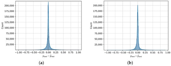
Figure 8.
Regression error distribution on the test dataset, along with its kernel density estimation, of the two best-performing regressors. (a) ANN. (b) Gradient Boosting.
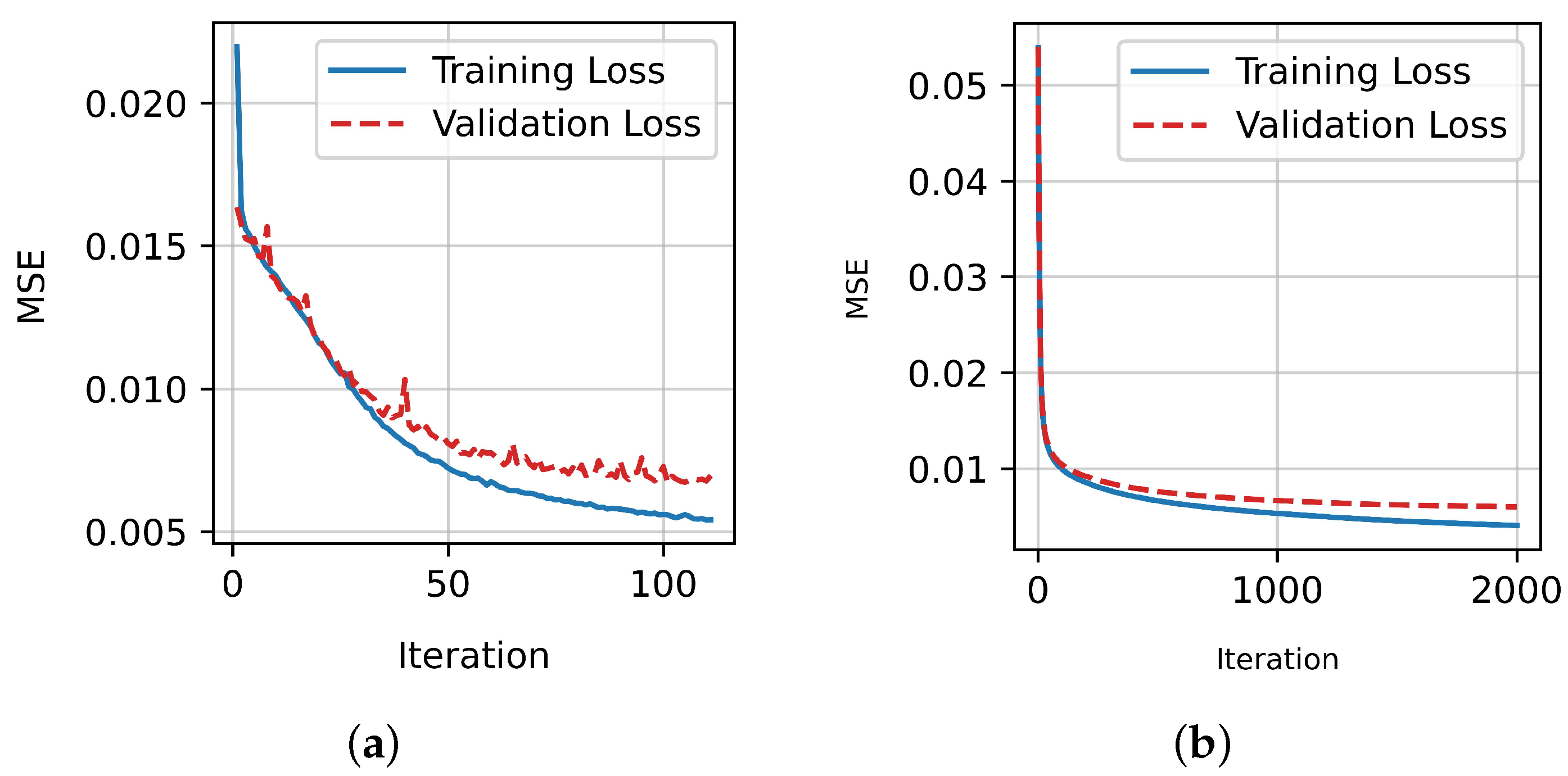
Finally, Figure 9 displays the evolution of the mean squared error of the two best-performing regressors. There is no significant gap between the loss on the training and validation datasets; thus, the algorithms did not overfit.
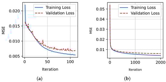
Figure 9.
Training loss curve of the two best-performing regressors. (a) Training loss curve of ANN. (b) Training loss curve of gradient boosting.
5. Summary and Conclusions
In the present paper, we applied ML algorithms to the problem of predicting the response of a rigid block under seismic excitation. On the one hand, we considered the problem of whether or not the block is overturning, and we used classification algorithms to approach it. On the other hand, we considered the problem of predicting the maximum rotation of the block in the cases where it does not overturn, and we used regression algorithms for our modeling. Departing from previously established literature, we predicted this maximum rotation directly instead of computing the whole time history of the rotation.
We obtained a classification accuracy on our test dataset of . That indicates the overall success of the algorithm to accurately assess the safety of the rigid rocking block under seismic excitation. In addition, the classification metrics are approximately equal for both classes, enhancing the reliability of the predictions. Finally, the algorithms exhibited no overfitting since the training and validation loss curves are very close. That indicates that the model generalizes well and its predictions are reliable on completely unseen data.
Similarly, for the regression task, we obtained an , with a mean absolute error of on the test dataset. The RMSE was higher (≈0.078), and this is due to the presence of a few very large errors. However, we observed that the model is unbiased, i.e., both the mean and median of the errors are very close to 0. In addition, the errors appear to be symmetrically distributed around 0, and in conjunction with the absence of bias, this implies that the model does not systematically over or underestimate the true values. Finally, similar to the classification task, Figure 9 demonstrates that there is no overfitting in the model; thus, its predictions are reliable on completely unseen data.
Overall, the results are encouraging and support the applicability of such methods to dynamic analysis problems, without the need to perform time-consuming and computationally intensive simulations. Since the rocking phenomenon is highly sensitive to parameters’ variation, the design of these systems should be treated probabilistically. From this point of view, the trained model can be used to rapidly generate a vast amount of response data to evaluate seismic fragility, which is a key component for seismic design and assessment. Potential future research steps could include the analysis of patterns on the misclassified input vectors, or cases where the regression error is very large. That could improve the already very good performance of the algorithms. Finally, the applicability of this method to similar dynamic problems could also be explored.
Author Contributions
Conceptualization, K.E.B. and I.E.K.; methodology, I.K., K.E.B., I.E.K., L.I. and A.E.; software, I.K., K.E.B., I.E.K., L.I. and A.E.; validation, I.K., K.E.B. and I.E.K.; formal analysis, I.K. and K.E.B.; investigation, I.K., K.E.B., I.E.K., L.I. and A.E.; resources, I.E.K., L.I. and A.E.; data curation, I.K., K.E.B., I.E.K., L.I. and A.E.; writing—original draft preparation, I.K., K.E.B. and I.E.K.; writing—review and editing, A.E. and L.I.; visualization, I.K. and K.E.B.; supervision L.I. and A.E. All authors have read and agreed to the published version of the manuscript.
Funding
This research received no external funding.
Institutional Review Board Statement
Not applicable.
Informed Consent Statement
Not applicable.
Data Availability Statement
The data that support the findings of this study are available upon reasonable request. The data are not publicly available due to confidentiality and privacy considerations.
Conflicts of Interest
The authors declare no conflicts of interest.
Abbreviations
The following abbreviations are used in this manuscript:
| ML | machine learning |
| DT | decision tree |
| ReLU | rectified linear unit |
| EDP | engineering demand parameter |
| ANN | artificial neural network |
| COR | coefficient of restitution |
| IM | intensity measure |
| PGA | peak ground acceleration |
| PGV | peak ground velocity |
| PGD | peak ground displacement |
| CAV | cumulative absolute velocity |
| CAD | cumulative absolute displacement |
| RMSE | root mean squared error |
| MAE | mean absolute error |
| MAPE | mean absolute percentage error |
| AUC | area under curve |
References
- Housner, G.W. The behavior of inverted pendulum structures during earthquakes. Bull. Seismol. Soc. Am. 1963, 53, 403–417. [Google Scholar] [CrossRef]
- Makris, N. A half-century of rocking isolation. Earthq. Struct. 2014, 7, 1187–1221. [Google Scholar] [CrossRef]
- Gelagoti, F.; Kourkoulis, R.; Anastasopoulos, I.; Gazetas, G. Rocking isolation of low-rise frame structures founded on isolated footings. Earthq. Eng. Struct. Dyn. 2012, 41, 1177–1197. [Google Scholar] [CrossRef]
- Agalianos, A.; Psychari, A.; Vassiliou, M.F.; Stojadinovic, B.; Anastasopoulos, I. Comparative assessment of two rocking isolation techniques for a motorway overpass bridge. Front. Built Environ. 2017, 3, 47. [Google Scholar] [CrossRef]
- Giouvanidis, A.I.; Dimitrakopoulos, E.G. Seismic performance of rocking frames with flag-shaped hysteretic behavior. J. Eng. Mech. 2017, 143, 04017008. [Google Scholar] [CrossRef]
- Makris, N.; Aghagholizadeh, M. The dynamics of an elastic structure coupled with a rocking wall. Earthq. Eng. Struct. Dyn. 2017, 46, 945–962. [Google Scholar] [CrossRef]
- He, X.; Unjoh, S.; Yamazaki, S.; Noro, T. Development of a bidirectional rocking isolation bearing system (Bi-RIBS) to control excessive seismic response of bridge structures. Earthq. Eng. Struct. Dyn. 2023, 52, 3074–3096. [Google Scholar] [CrossRef]
- Wada, A.; Qu, Z.; Motoyui, S.; Sakata, H. Seismic retrofit of existing SRC frames using rocking walls and steel dampers. Front. Archit. Civ. Eng. China 2011, 5, 259–266. [Google Scholar] [CrossRef]
- Ríos-García, G.; Benavent-Climent, A. New rocking column with control of negative stiffness displacement range and its application to RC frames. Eng. Struct. 2020, 206, 110133. [Google Scholar] [CrossRef]
- Bachmann, J.; Vassiliou, M.F.; Stojadinović, B. Dynamics of rocking podium structures. Earthq. Eng. Struct. Dyn. 2017, 46, 2499–2517. [Google Scholar] [CrossRef]
- Bantilas, K.E.; Kavvadias, I.E.; Vasiliadis, L.K. Seismic response of elastic multidegree of freedom oscillators placed on the top of rocking storey. Earthq. Eng. Struct. Dyn. 2021, 50, 1315–1333. [Google Scholar] [CrossRef]
- Bantilas, K.E.; Kavvadias, I.E.; Vasiliadis, L.K. Analytical investigation of the seismic response of elastic oscillators placed on the top of rocking storey. Bull. Earthq. Eng. 2021, 19, 1249–1270. [Google Scholar] [CrossRef]
- Bantilas, K.E.; Kavvadias, I.E.; Elenas, A. Analytical modeling and seismic performance of a novel energy dissipative kinematic isolation for building structures. Eng. Struct. 2023, 294, 116777. [Google Scholar] [CrossRef]
- Kazantzi, A.; Lachanas, C.; Vamvatsikos, D. Seismic response distribution expressions for rocking building contents under ordinary ground motions. Bull. Earthq. Eng. 2022, 20, 6659–6682. [Google Scholar] [CrossRef]
- Liu, P.; Zhang, Y.M.; Chen, H.T.; Yang, W.G. Experimental study on rocking blocks subjected to bidirectional ground and floor motions via shaking table tests. Earthq. Eng. Struct. Dyn. 2023, 52, 3171–3192. [Google Scholar] [CrossRef]
- Fragiadakis, M.; Diamantopoulos, S. Fragility and risk assessment of freestanding building contents. Earthq. Eng. Struct. Dyn. 2020, 49, 1028–1048. [Google Scholar] [CrossRef]
- Ruggieri, S.; Vukobratović, V. Acceleration demands in single-storey RC buildings with flexible diaphragms. Eng. Struct. 2023, 275, 115276. [Google Scholar] [CrossRef]
- Vukobratović, V.; Ruggieri, S. Floor acceleration demands in a twelve-storey RC shear wall building. Buildings 2021, 11, 38. [Google Scholar] [CrossRef]
- Acikgoz, S.; DeJong, M.J. The interaction of elasticity and rocking in flexible structures allowed to uplift. Earthq. Eng. Struct. Dyn. 2012, 41, 2177–2194. [Google Scholar] [CrossRef]
- Vassiliou, M.F.; Truniger, R.; Stojadinović, B. An analytical model of a deformable cantilever structure rocking on a rigid surface: Development and verification. Earthq. Eng. Struct. Dyn. 2015, 44, 2775–2794. [Google Scholar] [CrossRef]
- Makris, N.; Vassiliou, M.F. Planar rocking response and stability analysis of an array of free-standing columns capped with a freely supported rigid beam. Earthq. Eng. Struct. Dyn. 2013, 42, 431–449. [Google Scholar] [CrossRef]
- Dimitrakopoulos, E.G.; Giouvanidis, A.I. Seismic response analysis of the planar rocking frame. J. Eng. Mech. 2015, 141, 04015003. [Google Scholar] [CrossRef]
- Yim, C.S.; Chopra, A.K.; Penzien, J. Rocking response of rigid blocks to earthquakes. Earthq. Eng. Struct. Dyn. 1980, 8, 565–587. [Google Scholar] [CrossRef]
- Bachmann, J.; Strand, M.; Vassiliou, M.F.; Broccardo, M.; Stojadinović, B. Is rocking motion predictable? Earthq. Eng. Struct. Dyn. 2018, 47, 535–552. [Google Scholar] [CrossRef]
- Giouvanidis, A.I.; Dimitrakopoulos, E.G. Rocking amplification and strong-motion duration. Earthq. Eng. Struct. Dyn. 2018, 47, 2094–2116. [Google Scholar] [CrossRef]
- Lachanas, C.G.; Vamvatsikos, D.; Dimitrakopoulos, E.G. Statistical property parameterization of simple rocking block response. Earthq. Eng. Struct. Dyn. 2023, 52, 394–414. [Google Scholar] [CrossRef]
- Sieber, M.; Vassiliou, M.F.; Anastasopoulos, I. Intensity measures, fragility analysis and dimensionality reduction of rocking under far-field ground motions. Earthq. Eng. Struct. Dyn. 2022, 51, 3639–3657. [Google Scholar] [CrossRef]
- Kavvadias, I.E.; Vasiliadis, L.K.; Elenas, A. Seismic response parametric study of ancient rocking columns. Int. J. Archit. Herit. 2017, 11, 791–804. [Google Scholar] [CrossRef]
- Dimitrakopoulos, E.G.; Paraskeva, T.S. Dimensionless fragility curves for rocking response to near-fault excitations. Earthq. Eng. Struct. Dyn. 2015, 44, 2015–2033. [Google Scholar] [CrossRef]
- Solarino, F.; Giresini, L. Fragility curves and seismic demand hazard analysis of rocking walls restrained with elasto-plastic ties. Earthq. Eng. Struct. Dyn. 2021, 50, 3602–3622. [Google Scholar] [CrossRef]
- Kavvadias, I.E.; Papachatzakis, G.A.; Bantilas, K.E.; Vasiliadis, L.K.; Elenas, A. Rocking spectrum intensity measures for seismic assessment of rocking rigid blocks. Soil Dyn. Earthq. Eng. 2017, 101, 116–124. [Google Scholar] [CrossRef]
- Wen, W.; Zhang, C.; Zhai, C. Rapid seismic response prediction of RC frames based on deep learning and limited building information. Eng. Struct. 2022, 267, 114638. [Google Scholar] [CrossRef]
- Lazaridis, P.C.; Kavvadias, I.E.; Demertzis, K.; Iliadis, L.; Vasiliadis, L.K. Interpretable Machine Learning for Assessing the Cumulative Damage of a Reinforced Concrete Frame Induced by Seismic Sequences. Sustainability 2023, 15, 12768. [Google Scholar] [CrossRef]
- Hwang, S.H.; Mangalathu, S.; Shin, J.; Jeon, J.S. Machine learning-based approaches for seismic demand and collapse of ductile reinforced concrete building frames. J. Build. Eng. 2021, 34, 101905. [Google Scholar] [CrossRef]
- Zahra, F.; Macedo, J.; Málaga-Chuquitaype, C. Hybrid data-driven hazard-consistent drift models for SMRF. Earthq. Eng. Struct. Dyn. 2023, 52, 1112–1135. [Google Scholar] [CrossRef]
- Nguyen, H.D.; Dao, N.D.; Shin, M. Prediction of seismic drift responses of planar steel moment frames using artificial neural network and extreme gradient boosting. Eng. Struct. 2021, 242, 112518. [Google Scholar] [CrossRef]
- Kazemi, F.; Asgarkhani, N.; Jankowski, R. Predicting seismic response of SMRFs founded on different soil types using machine learning techniques. Eng. Struct. 2023, 274, 114953. [Google Scholar] [CrossRef]
- Junda, E.; Málaga-Chuquitaype, C.; Chawgien, K. Interpretable machine learning models for the estimation of seismic drifts in CLT buildings. J. Build. Eng. 2023, 70, 106365. [Google Scholar] [CrossRef]
- Soleimani, F. Probabilistic seismic analysis of bridges through machine learning approaches. Structures 2022, 38, 157–167. [Google Scholar] [CrossRef]
- Deng, Z.; Huang, M.; Wan, N.; Zhang, J. The Current Development of Structural Health Monitoring for Bridges: A Review. Buildings 2023, 13, 1360. [Google Scholar] [CrossRef]
- Mangalathu, S.; Sun, H.; Nweke, C.C.; Yi, Z.; Burton, H.V. Classifying earthquake damage to buildings using machine learning. Earthq. Spectra 2020, 36, 183–208. [Google Scholar] [CrossRef]
- Zhang, H.; Cheng, X.; Li, Y.; He, D.; Du, X. Rapid seismic damage state assessment of RC frames using machine learning methods. J. Build. Eng. 2023, 65, 105797. [Google Scholar] [CrossRef]
- Yuan, X.; Chen, G.; Jiao, P.; Li, L.; Han, J.; Zhang, H. A neural network-based multivariate seismic classifier for simultaneous post-earthquake fragility estimation and damage classification. Eng. Struct. 2022, 255, 113918. [Google Scholar] [CrossRef]
- Kiani, J.; Camp, C.; Pezeshk, S. On the application of machine learning techniques to derive seismic fragility curves. Comput. Struct. 2019, 218, 108–122. [Google Scholar] [CrossRef]
- Dabiri, H.; Faramarzi, A.; Dall’Asta, A.; Tondi, E.; Micozzi, F. A machine learning-based analysis for predicting fragility curve parameters of buildings. J. Build. Eng. 2022, 62, 105367. [Google Scholar] [CrossRef]
- Liu, Z.; Sextos, A.; Guo, A.; Zhao, W. ANN-based rapid seismic fragility analysis for multi-span concrete bridges. Structures 2022, 41, 804–817. [Google Scholar] [CrossRef]
- Gerolymos, N.; Apostolou, M.; Gazetas, G. Neural network analysis of overturning response under near-fault type excitation. Earthq. Eng. Eng. Vib. 2005, 4, 213–228. [Google Scholar] [CrossRef]
- Pan, X.; Wen, Z.; Yang, T. Dynamic analysis of nonlinear civil engineering structures using artificial neural network with adaptive training. arXiv 2021, arXiv:2111.13759. [Google Scholar]
- Achmet, Z.; Diamantopoulos, S.; Fragiadakis, M. Rapid seismic response prediction of rocking blocks using machine learning. Bull. Earthq. Eng. 2023, 1–19. [Google Scholar] [CrossRef]
- Shen, Y.; Málaga-Chuquitaype, C. Physics-informed AI models for the seismic response prediction of rocking structures. Data-Centric Eng. 2023. under publication. [Google Scholar]
- Brown, L.T.; Diehl, J.G.; Nigbor, R.L. A simplified procedure to measure average shear-wave velocity to a depth of 30 meters (VS30). In Proceedings of the 12th World Conference on Earthquake Engineering, Auckland, New Zealand, 30 January–4 February 2000; pp. 1–8. [Google Scholar]
- Trifunac, M.D.; Brady, A.G. A study on the duration of strong earthquake ground motion. Bull. Seismol. Soc. Am. 1975, 65, 581–626. [Google Scholar]
- Maheshwari, S.; Jain, R.; Jadon, R. A review on class imbalance problem: Analysis and potential solutions. Int. J. Comput. Sci. Issues 2017, 14, 43–51. [Google Scholar]
- Satyasree, K.; Murthy, J. An exhaustive literature review on class imbalance problem. Int. J. Emerg. Trends Technol. Comput. Sci. 2013, 2, 109–118. [Google Scholar]
- Meskouris, K. Structural Dynamics: Models, Methods, Examples; Ernst & Sohn: Hoboken, NJ, USA, 2000. [Google Scholar]
- Rathje, E.M.; Abrahamson, N.A.; Bray, J.D. Simplified frequency content estimates of earthquake ground motions. J. Geotech. Geoenviron. Eng. 1998, 124, 150–159. [Google Scholar] [CrossRef]
- Kramer, S.L. Geotechnical Earthquake Engineering; Pearson Education India: Bangalore, India, 1996. [Google Scholar]
- Papasotiriou, A.; Athanatopoulou, A. Seismic intensity measures optimized for low-rise reinforced concrete frame structures. J. Earthq. Eng. 2022, 26, 7587–7625. [Google Scholar] [CrossRef]
- Dimitrakopoulos, E.; Kappos, A.J.; Makris, N. Dimensional analysis of yielding and pounding structures for records without distinct pulses. Soil Dyn. Earthq. Eng. 2009, 29, 1170–1180. [Google Scholar] [CrossRef]
- Arias, A. A Measure of Earthquake Intensity; MIT Press: Cambridge, MA, USA, 1970. [Google Scholar]
- Ang, A. Reliability bases for seismic safety assessment and design. In Proceedings of the 4th US National Conference on Earthquake Engineering, Palm Springs, CA, USA, 20–24 May 1990; Earthquake Engineering Research Institute: Oakland, CA, USA, 1990; Volume 1, pp. 29–45. [Google Scholar]
- Fajfar, P.; Vidic, T.; Fischinger, M. A measure of earthquake motion capacity to damage medium-period structures. Soil Dyn. Earthq. Eng. 1990, 9, 236–242. [Google Scholar] [CrossRef]
- Cabanas, L.; Benito, B.; Herráiz, M. An approach to the measurement of the potential structural damage of earthquake ground motions. Earthq. Eng. Struct. Dyn. 1997, 26, 79–92. [Google Scholar] [CrossRef]
- Kotsiantis, S.B.; Zaharakis, I.; Pintelas, P. Supervised machine learning: A review of classification techniques. Emerg. Artif. Intell. Appl. Comput. Eng. 2007, 160, 3–24. [Google Scholar]
- Fernández-Delgado, M.; Sirsat, M.S.; Cernadas, E.; Alawadi, S.; Barro, S.; Febrero-Bande, M. An extensive experimental survey of regression methods. Neural Netw. 2019, 111, 11–34. [Google Scholar] [CrossRef]
- Cilimkovic, M. Neural Networks and Back Propagation Algorithm; Institute of Technology Blanchardstown: Dublin, Ireland, 2015; Volume 15. [Google Scholar]
- Vanschoren, J. Meta-learning: A survey. arXiv 2018, arXiv:1810.03548. [Google Scholar]
- Kingsford, C.; Salzberg, S.L. What are decision trees? Nat. Biotechnol. 2008, 26, 1011–1013. [Google Scholar] [CrossRef] [PubMed]
- Natekin, A.; Knoll, A. Gradient boosting machines, a tutorial. Front. Neurorobot. 2013, 7, 21. [Google Scholar] [CrossRef] [PubMed]
- Ramjee, S.; Wornow, M. Histogram-Based Gradient Boosting Trees for Efficient Graph Learning with Wasserstein Embeddings. Available online: https://sharanramjee.github.io/files/projects/cs224w.pdf (accessed on 25 December 2023).
- Alsabti, K.; Ranka, S.; Singh, V. CLOUDS: A Decision Tree Classifier for Large Datasets. In Proceedings of the Fourth International Conference on Knowledge Discovery & Data Mining (KDD-98), New York, NY, USA, 27–31 August 1998. [Google Scholar]
- Ke, G.; Meng, Q.; Finley, T.; Wang, T.; Chen, W.; Ma, W.; Ye, Q.; Liu, T.Y. Lightgbm: A highly efficient gradient boosting decision tree. Adv. Neural Inf. Process. Syst. 2017, 30, 3149–3157. [Google Scholar]
- Pedregosa, F.; Varoquaux, G.; Gramfort, A.; Michel, V.; Thirion, B.; Grisel, O.; Blondel, M.; Prettenhofer, P.; Weiss, R.; Dubourg, V.; et al. Scikit-learn: Machine Learning in Python. J. Mach. Learn. Res. 2011, 12, 2825–2830. [Google Scholar]
- Loh, W.Y. Classification and regression trees. Wiley Interdiscip. Rev. Data Min. Knowl. Discov. 2011, 1, 14–23. [Google Scholar] [CrossRef]
- Ahsan, M.M.; Mahmud, M.P.; Saha, P.K.; Gupta, K.D.; Siddique, Z. Effect of Data Scaling Methods on Machine Learning Algorithms and Model Performance. Technologies 2021, 9, 52. [Google Scholar] [CrossRef]
- Yang, L.; Shami, A. On hyperparameter optimization of machine learning algorithms: Theory and Practice. Neurocomputing 2020, 415, 295–316. [Google Scholar] [CrossRef]
- Raschka, S. An overview of general performance metrics of binary classifier systems. arXiv 2014, arXiv:1410.5330. [Google Scholar]
Disclaimer/Publisher’s Note: The statements, opinions and data contained in all publications are solely those of the individual author(s) and contributor(s) and not of MDPI and/or the editor(s). MDPI and/or the editor(s) disclaim responsibility for any injury to people or property resulting from any ideas, methods, instructions or products referred to in the content. |
© 2023 by the authors. Licensee MDPI, Basel, Switzerland. This article is an open access article distributed under the terms and conditions of the Creative Commons Attribution (CC BY) license (https://creativecommons.org/licenses/by/4.0/).