Abstract
To address the issue of low positioning accuracy in unmanned vehicles navigating in obstructed spaces due to easily contaminated navigation measurement information, an improved adaptive federated Kalman filtering INS/GNSS/VNS integrated navigation algorithm is proposed. In this algorithm, an inertial navigation system (INS) serves as the common reference system, and, together with the global navigation satellite system (GNSS) and visual navigation system (VNS), they form the subsystems that together make up the main system. In the event of faulty measurement values in the subsystems, a combination of the residual chi-square and sliding-window averaging methods are used for fault detection to improve the fault tolerance of the integrated navigation algorithm. Additionally, an adaptive sharing factor is proposed to adjust the accuracy of the integrated navigation algorithm based on the accuracy of the sub-filters. Simulation experiments demonstrated that, compared with classic federated Kalman filtering, the proposed algorithm reduced the root mean square errors (RMSEs) of the three-dimensional position by 56.4%, 54.8%, and 43.4% and the root mean square errors of the three-dimensional velocity by 71.0%, 72.1%, and 28.4% in the event of sub-filter faults, effectively solving the problem of low positioning accuracy for unmanned vehicles in obstructed spaces while ensuring the real-time performance of the system.
1. Introduction
In recent years, with the rapid development of unmanned autonomous systems, the application fields of unmanned vehicles have become increasingly extensive. After major natural disasters, buildings such as houses and bridges may collapse, forming a sheltered space. Due to the complex environment and narrow and dim space, satellite signals are easily interfered with or blocked, which often leads to the failure of the navigation and positioning of unmanned vehicles in the sheltered space. Therefore, providing accurate, reliable, and real-time navigation information such as position, velocity, and attitude for unmanned vehicles in obstructed spaces is an important guarantee for obtaining disaster information and improving search and rescue efficiency and has significant importance.
Inertial navigation systems (INSs) [1] have the advantages of small size, easy integration, and pure autonomy, and they are widely used in various navigation fields. However, the errors [2,3] of INSs accumulate rapidly over time. INS/GNSS [4,5,6] can obtain higher-precision carrier velocity and position information using the global navigation satellite system [7] (GNSS). Visual navigation systems [8,9] (VNSs) can obtain the high-precision attitude information of a carrier, but they suffer from the drawbacks of increased measurement error in environments with insufficient feature points or significant changes in illumination. Therefore, combining INS, GNSS, and VNS can compensate for their respective shortcomings and further improve the positioning accuracy [10] of unmanned vehicle navigation systems in complex scenarios.
A centralized Kalman filter [11,12,13] can achieve multi-source fusion navigation using the effective information from various sensors for optimal estimation, thus achieving a higher positioning accuracy. However, as the dimension of the state vector increases, the consumption of computational resources increases, and real-time performance deteriorates. Carlson et al. [14,15] proposed a federated Kalman filter [16,17] (FKF), which utilizes the principle of information distribution, not only reducing the computational load but also improving the fault-tolerant performance of integrated navigation. In an FKF, all sub-filters evenly distribute the information sharing factor (ISF) [11,18,19] for information sharing. However, in practical applications, the performance and estimation accuracy of subsystems constantly change with the complexity of the navigation environment, and the fixed ISF in an FKF cannot meet the different navigation requirements of the navigation system in complex scenarios.
Lu et al. [20] combined an odometer with an INS/GPS integrated navigation system and proposed a strategy of using an adaptive information allocation factor, which improved the disturbance rejection capability of the integrated navigation system. Xu et al. [21] used a dual-state chi-square detection algorithm to calculate the parameters corresponding to each state, ensuring that states with a higher accuracy obtain a larger information distribution coefficient. Zhai et al. [22] proposed an adjustment strategy using a degree of abnormality to correct the error covariance matrix and Kalman gain, which improved the fault tolerance and accuracy of the positioning system. Shen et al. [23] proposed a time-varying information sharing factor adaptive federated Kalman filter. In a complex GNSS environment, the proposed adaptive information fusion strategy could autonomously adjust the information sharing factors and their error states of each navigation sensor. Lyu et al. [24] developed a novel adaptive federated interacting multiple model (IMM) filter for autonomous underwater vehicle integrated navigation systems. The information sharing coefficients of the adaptive federated IMM filter are dynamically adjusted based on the performance of each local system, ensuring the optimal fusion of information from different sources. Xu et al. [25] developed a robust adaptive federal unscented Kalman filter (RAFUKF) SINS/GNSS/VDM combined navigation algorithm. A federal unscented Kalman filter (FUKF) framework was developed to combine the filter variance with the f-parameter to construct a new ISF and to establish quantitative estimation fault detection mechanisms. Dai et al. [26] proposed a robust adaptive localization algorithm that utilizes a robust equivalent weight estimation sub-filter and adaptively allocates the information sharing coefficient using the sub-filter state covariance. Jiang et al. [18] proposed a GPS-AOA-SINS integrated positioning scheme with fault detection inserted between the sub-filter and the main filter. The gain matrix of the fault sub-filter is adjusted in real-time to reduce its impact on the entire system. Chen et al. [27] improved the filtering accuracy and system stability by constructing a confidence test model to effectively filter out faulty measurement information and adjusting the system noise covariance in real time. Xiong et al. [28] constructed a simplified state chi-square test(SSCST) for fault detection by using the residuals between actual and predicted observations, and they incorporated a time-varying decay factor into the sub-filters to enhance the stability of the system.
However, most of these studies focused on specific scenarios and single-sensor anomalies, and they lack a discussion on complex and dynamic scenarios [16], as well as different types of sensor failures. In this paper, an improved adaptive federated filter (IAFKF) algorithm based on a federated Kalman filter was designed for the combination navigation system of INS/GNSS/VNS, which is used for unmanned vehicles in obstructed spaces. INS/GNSS and INS/VNS fusion navigation models are established. In the event of possible GNSS and VNS failures, a fault detection algorithm combining the residual chi-square and sliding-window average methods is proposed, which can better detect and isolate fault signals. An adaptive information sharing factor is also proposed to improve the positioning accuracy and fault tolerance by adjusting the error covariance matrix. Finally, the effectiveness of the proposed improved AFKF algorithm was verified through simulation experiments.
The structure of this paper is as follows: In Section 2, a multi-source fusion model based on federated Kalman filtering is established by combining INS/GNSS and INS/VNS fusion navigation models. In Section 3, a fault detection method combining the residual chi-square test and sliding-window averaging and an adaptive information sharing factor are proposed. In Section 4, the effectiveness and real-time performance of the proposed integrated navigation algorithm are verified through simulation experiments. Finally, conclusions are drawn in Section 5.
2. Multi-Source Fusion Model
Figure 1 shows the structure of the INS/GNSS/VNS integrated navigation system [29,30]. The system uses INS as the main filter and reference system for the sub-filters, which utilize observation information from the external observation system GNSS and the autonomous observation system VNS to construct sub-filter 1 and sub-filter 2. The INS estimates the position, velocity, and attitude, and the sub-filter observation information is used to correct the system state to obtain a local optimal estimate. The global optimal estimate of the system state is then obtained through global fusion by the main filter.
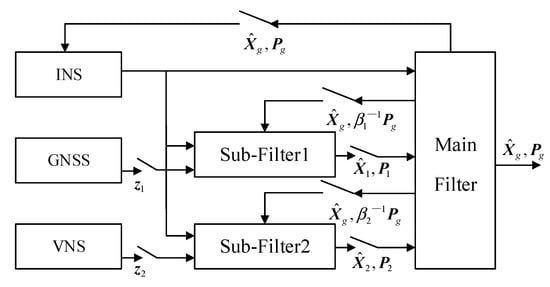
Figure 1.
The structure of the INS/GNSS/VNS integrated navigation system.
2.1. Integrated Navigation Systems and Error Models
The navigation coordinate system is defined as an east–north–up (E-N-U) coordinate system. In this case, the system state vector is as follows:
where are the attitude angle errors, are the velocity errors, are the longitude, latitude, and altitude errors, are the gyro drift errors, and are the accelerometer drift errors. By analyzing the errors of the inertial navigation system, the error state equation is obtained as follows:
where is the state transition matrix of the inertial navigation system from time k − 1 to k, is the error state vector at time k, is the error state vector at time k − 1, is the noise coefficient matrix, and is the system noise vector.
2.2. Measurement Equation of System
After establishing the error state equation of the integrated navigation system, a measurement equation is required to update the attitude angle, velocity, and position of the integrated navigation system. GNSS can observe the velocity and position information of the unmanned vehicle, while VNS can observe the attitude angle of the unmanned vehicle. The velocity and position information of INS and GNSS were selected as the measurement vector to establish the sub-filter 1 of INS/GNSS, and the attitude angle information of INS and VNS was selected as the measurement vector to establish the sub-filter 2 of INS/VNS.
For the measurement equation, we usually use the following discrete time expressions:
where is the measurement vector, is the measurement matrix, and is the measurement noise vector, which is typically modeled as zero-mean Gaussian white noise.
In the INS/GNSS integrated navigation, the GNSS provides measurements of the position and velocity. The measurement equation for the INS/GNSS integration is as follows:
where represents the measurement noise vector of GNSS, which is modeled as independent zero-mean Gaussian white noise, and represents the measurement matrix of GNSS, which can be expressed as:
In the INS/VNS integrated navigation system, the visual navigation system provides measurements of the attitude. The measurement equation for the INS/VNS integration is as follows:
where represents the attitude measurement noise vector of VNS, which is modeled as independent zero-mean Gaussian white noise, and represents the measurement matrix of VNS, which can be expressed as:
To clearly represent the information processing process of each sub-filter in the federated Kalman filter, it can be assumed that the model of the sub-filter is as follows:
where is the state vector of the i-th sub-filter at time k, is the state transition matrix of the i-th sub-filter, is the noise transition matrix of the i-th sub-filter at time k − 1, and is the system noise matrix. represents the measurement value, represents the measurement matrix of the sub-filter, and represents the measurement noise vector of the sub-filter.
Time update: This is a process of a one-step prediction state update and a one-step prediction error covariance update:
where represents the covariance matrix of the input system noise vector , represents the error covariance matrix at time k − 1, and represents the one-step prediction error covariance matrix from time k − 1 to k.
Measurement update: The optimal Kalman gain for the sub-filter is as follows.
The covariance matrix of the measurement noise vector is .
Therefore, the posterior state estimate is as follows:
The posterior estimate error covariance is as follows:
Information fusion: The global optimal estimation is obtained through the estimation results of all the sub-filters:
Information sharing process: Finally, the fused results are allocated to the individual sub-filters according to the following formula, which is used as the initial value for the sub-filter at the next moment:
where represents the allocation coefficient of the i-th sub-filter, and the subscript ‘g’ indicates the main filter. According to the principle of information distribution proposed by Carlson [15], the information sharing factor should satisfy the condition of information conservation:
3. Improved Adaptive Federated Kalman Filter (IAFKF)
In obstructed spaces, GNSS is prone to positioning anomalies or even satellite unavailability, resulting in a decrease in the positioning accuracy of the integrated navigation system. Additionally, visual navigation systems have poor performance in cloudy or dark environments. Furthermore, since the estimated state values of the federated Kalman sub-filters are fed back to each sub-filter after global fusion by the main filter, the other sub-filters are further contaminated, resulting in positioning errors or even divergence. Therefore, this paper introduces fault detection between the sub-filters and the main filter to detect and process faults in real-time, improving the overall navigation accuracy and fault tolerance.
3.1. Fault Detection
According to the Kalman filter equation, the recursive value at time k is derived from the previous time k − 1:
The measurement residual is as follows [26]:
In this equation, represents the measurement residual of the i-th sub-filter at time k in distributed filtering. When there is no fault in the system, the residual follows a Gaussian white noise distribution with a mean of 0, and its covariance matrix is as follows:
A fault detection statistic based on the characteristics of the chi-squared distribution can be constructed as follows:
In this equation, follows a chi-squared distribution with m degrees of freedom (the dimension of the measurement Z). If a fault occurs, the residual will no longer be a zero-mean white noise process, and therefore the following method can be used to detect faults.
The fault detection criteria are as follows:
In this context, represents the fault detection threshold, and represents the fault flag at time k. When , the measurement system has a fault and requires isolation processing. When , the measurement system is functioning normally. The value of can be calculated based on Equation (25) and the degree of freedom m and confidence level using a chi-squared distribution table:
To eliminate occasional abnormal situations, a sliding-window average can be applied to the residual sequence to obtain the actual residual covariance:
Here, represents the estimated value of the prediction error covariance matrix within the calculation interval N. The specific value of N is determined based on experience and the specific situation and is generally chosen to be between 10 and 12. By comparing the trace of the actual covariance of the residuals and the theoretical covariance, we can assess the degree of deviation between the true value and the theoretical value.
where, is the degree of deviation between the real value and the theoretical value. When the actual covariance of the residuals is generally consistent with the theoretical covariance, is generally considered to be an indication of a fault-free measurement system. When the actual covariance of the residuals differs significantly from the theoretical covariance, i.e., when , it is considered to be an indication of a fault in the measurement system.
In this paper, the above two methods are used for fault detection to avoid false alarms or missed detections, thereby reducing the impact of fault signals on the system. If the measurement system fails, the entire system’s state information will be affected after the fusion of the main filter information. In order to ensure the normal stability of the system and avoid the isolation of sub-filters affecting the overall system, a simple compensation method was chosen. That is, when a fault is detected, the estimate of the main filter is used instead of the estimate of the faulty sub-filter.
3.2. Adaptive Information Sharing Factor
In a classic FKF [14], the information sharing factor is evenly allocated among all the sub-filters. However, this equal distribution method neglects the unique characteristics of each sub-filter, which can result in errors from some sub-filters impacting the positioning accuracy of the main filter. Improper allocation of the information sharing factor can also decrease the accuracy of the integrated navigation system. Therefore, an adaptive allocation of the information sharing factor based on the characteristics of each sub-filter is crucial for improving their performance. To address this issue, this paper proposes an adaptive information sharing factor that can be dynamically allocated based on the state covariance matrix of each sub-filter, reducing the impact of low-precision sub-filters on the positioning accuracy of the main filter. In practical filtering, the state covariance matrix reflects the precision of the filter, where a smaller corresponds to a higher accuracy of the filter.
The relationship between the precision of the sub-filtering system in this paper and the state covariance is as follows:
where represents the filtering accuracy of the i-th sub-filter at time k, and tr represents the trace of the matrix. The adaptive information sharing coefficient can be expressed by the precision of the sub-filtering system as follows:
where represents the information sharing factor, and N represents the number of sub-filters. According to Equation (16), the information fusion state of the main filter is as follows:
3.3. Procedure of Improved AFKF
The procedure is shown below:
- Step 1: Set the initial values of the filter, including the initial state value , the system noise covariance , and the measurement noise covariance .
- Step 2: Time update: the sub-filter performs a time update as per Equations (10) and (11).
- Step 3: Measurement update: the sub-filter performs a measurement update as per Equations (12)–(14).
- Step 4: Fault detection: using the residual chi-square and sliding-window averaging method for fault detection, the estimated value of the faulty sub-filter is replaced with the estimated value of the main filter as per Equations (21)–(28).
- Step 5: Information fusion is carried out as per Equations (15) and (16).
- Step 6: Adaptive information sharing factor is calculated as per Equations (29)–(31).
- Step 7: Information sharing process is carried out as per Equations (17)–(20).
- Step 8: Steps 2 to 7 are repeated in a loop.
4. Simulation Experiment
To verify the effectiveness, fault tolerance, and real-time performance of the proposed improved AFKF for INS/GNSS/VNS integrated navigation, we conducted simulation experiments and compared them with a classic FKF. In the simulation experiments, we set different index parameters for the accelerometer, gyroscope, GNSS, and VNS, as shown in Table 1. At the same time, we also considered the complexity of the real environment in unmanned vehicle navigation and reasonably set the failure scenarios for GNSS and VNS. In the different scenarios, we compared and analyzed the performance of the different algorithms, and the simulation trajectories are shown in Figure 2. The running platform for this simulation experiment was an INTEL(R) Core (YM) I5-12500H CPU with 16.00 GB of memory, and the simulation software used was the PSINS toolbox under matlab2022a, which was developed by Professor Gongmin Yan from Northwestern Polytechnical University, which can be used for simulation experiments of integrated navigation systems.

Table 1.
Parameters in simulations.
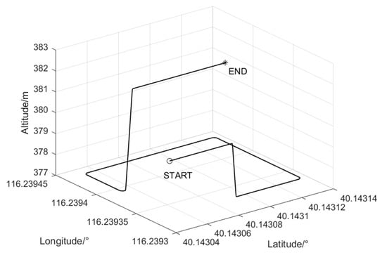
Figure 2.
Simulation trajectory.
The initial position (local coordinates) was set to , the initial attitude (pitch, roll, yaw) was set to , and the initial velocity (local coordinates) was set to [0 m/s, 0 m/s, 0 m/s]. This corresponded to a simulation of an unmanned vehicle going downhill, uphill, and around corners in an unmanned vehicle trajectory.
In order to simulate the complex environment that unmanned vehicles may encounter in obstructed spaces, we simulated two scenarios. Scenario 1 involved a situation where only the GNSS signal was interfered with or obscured. Scenario 2 involved a situation where both GNSS and VNS were interfered with.
4.1. Scenario 1
This scenario involved a simulation of the GNSS signal being subjected to different degrees of interference or occlusion during the driving of an unmanned vehicle in obstructed spaces. The two time periods were as follows:
Period 1: a time period between 250 s~400 s, where the GNSS signal was weakly interfered with or blocked, and a 10-fold measurement error was added to the GNSS positioning measurement, as shown in Equation (32):
Period 2: a time period between 600 s~750 s, where the GNSS signal was strongly interfered with or blocked, and a 20-fold measurement error was added to the GNSS positioning measurement, as shown in Equation (33):
Here, represents the true position information, represents the attitude error of the visual navigation, and represents a matrix of a standard normal distribution. The comparison between the improved AFKF proposed in this paper and a classic FKF is shown below. The results of the INS/GNSS/VNS integrated navigation position and velocity errors are shown in Figure 3a,b, and the three-axis position and velocity errors are listed in Table 2.
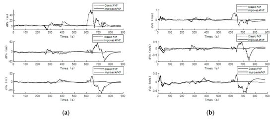
Figure 3.
Comparison of navigation errors between improved AFKF and classic FKF: (a) Comparison of position errors. (b) Comparison of velocity errors.
Table 2.
Navigation error statistics results of classic FKF and improved AFKF.
It can be seen that in periods 1 and 2, when the GNSS was subjected to different degrees of interference or obstruction, the improved AFKF proposed in this paper performed significantly better than the classic FKF. In all periods, compared with the classic FKF, the three-axis position average error of the improved AFKF decreased by 62.8%, 60.4%, 69.1%, and the three-axis velocity average error decreased by 79.7%, 77.9%, and 68.4%, respectively.
4.2. Scenario 2
Simulating the driving process of unmanned vehicles in an obstructed space may result in GNSS signal interference or blockage, as well as a shortage of feature points due to environmental issues in VNS. In this simulation, these situations occurred during different time periods.
Period 1: a time period between 250 s~400 s, where the unmanned vehicle drove into a dark scene where there were fewer feature points, which caused a malfunction in the visual navigation. Therefore, a 10-fold measurement error was introduced in the visual positioning. The following formula (34) shows this, where is the true position information, is the visual navigation position error, and is a matrix of the standard normal distribution:
Period 2: a time period between 600 s~750 s; considering that an unmanned vehicle may drive into certain areas with strong signal interference or obstructed spaces, which can cause GNSS navigation to fail, a 20-fold measurement error was introduced in the GNSS positioning. The following formula (35) shows this, where is the true position information, is the GNSS navigation velocity and position error, and is a matrix of the standard normal distribution:
The comparison between the improved AFKF proposed in this paper and a classic FKF is shown below. The position and velocity error results of the INS/GNSS/VNS integrated navigation are shown in Figure 4a,b, and the average errors of the position and velocity of the combined navigation are listed in Table 3.
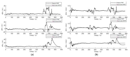
Figure 4.
Comparison of navigation errors between improved AFKF and FKF: (a) Comparison of position errors. (b) Comparison of velocity errors.
Table 3.
Navigation error statistics results of classic FKF and improved AFKF.
Through the analysis of the results shown in Figure 4a,b and Table 3, it was found that when the simulated unmanned vehicle experienced failures in satellite navigation and visual navigation during time periods 1 and 2, the improved AFKF proposed in this paper performed significantly better than the classic FKF. Without interference to the navigation signal, the improved AFKF showed a 35.4% reduction in the position error and a 54.8% reduction in the velocity error compared to the classic FKF. Across all the time periods, the improved AFKF exhibited an average reduction of 25.1% in the position error and 62.4% in the velocity error compared to the classic FKF.
In order to prevent the randomness of non-Gaussian noise and verify the adaptive and fault detection capabilities of the algorithm proposed in this paper, the system was subjected to 50 independent simulations in scenario 2, and the root mean square error (RMSE) of these 50 simulations was calculated as a performance metric. The definition of RMSE is as follows:
where N represents the experiment time, and and represent the true value and estimated value, respectively, of the state at time step k. The final results are shown in Figure 5a,b. The average root mean square position error and the average root mean square velocity error of the 50 simulation experiments are listed in Table 4.
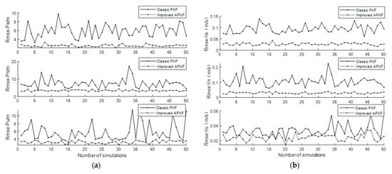
Figure 5.
RMSE of classic FKF and improved AFKF: (a) RMSE of position. (b) RMSE of velocity.
Table 4.
The mean RMSE of 50 simulation experiments.
From Figure 5a,b and Table 4, it can be seen that in these INS/GNSS/VNS integrated navigation simulation experiments, the position and velocity errors determined using the improved FKF proposed in this paper were significantly smaller than those using the classic FKF. The average root mean square errors of the position in the three directions of east, north, and up decreased by 56.4%, 54.8%, and 43.4%, respectively, and the average root mean square errors of the velocity in the three directions of east, north, and up decreased by 71.0%, 72.1%, and 28.4%, respectively.
In order to validate the real-time performance of the proposed improved AFKF algorithm, using the same simulation software and platform as described above and with the same raw data, we compared the entire filtering process time between the improved AFKF and the classic FKF in 50 simulation experiments, as shown in Figure 6. The driving time of the unmanned vehicle in the simulation was 887.5 s, with an average runtime of 11.2493 s for the improved AFKF and 10.3526 s for the classic FKF. Although the average runtime of the improved AFKF proposed in this paper was increased by 8.66% compared to the classic FKF, it still met the real-time requirements of the integrated navigation of unmanned vehicles. The filtering cycle of the improved AFKF was 1 s, and the INS update period was 0.02 s. The average filtering time was less than 3.69 ms, which was smaller than the INS update period, satisfying the real-time requirements of the system.
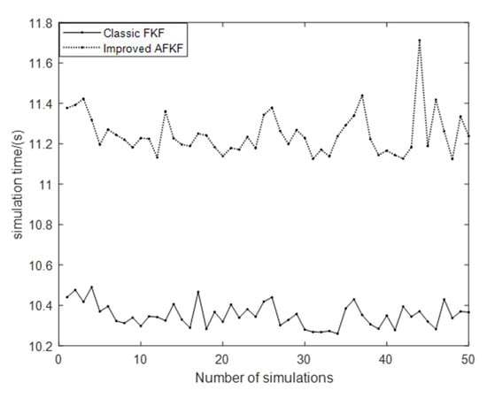
Figure 6.
Comparison chart of the running time for 50 simulation experiments.
To further verify the effectiveness of the algorithm, we conducted simulation experiments on the Gazebo platform, an open-source robot simulation platform that relies on the popular robot operating system (ROS), as shown in Figure 7a. The unmanned vehicle model used in the simulation experiment was the TurtleBot3-Waffle-Pi, which is a widely used open-source robot for research and education. It is small in size and highly scalable, and the main model parameters and movements used during the simulation are shown in Table 5. As shown in Figure 7b, an environment for the unmanned vehicle to travel in was constructed on the Gazebo platform, and the unmanned vehicle traveled at a constant speed of 0.26 m/s. The improved AFKF algorithm proposed in this paper was used to locate the movement of the unmanned vehicle, and the reference trajectory is shown in Figure 8.
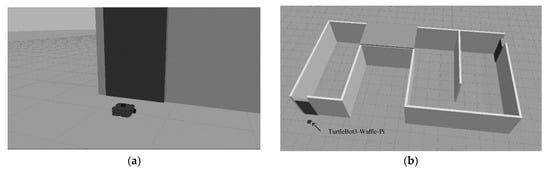
Figure 7.
Simulation experiments on the Gazebo platform: (a) Unmanned vehicle model TurtleBot3-Waffle-Pi. (b) Environment for unmanned vehicle travel.
Table 5.
The main model parameters in simulation.
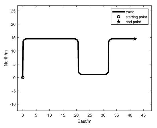
Figure 8.
Reference trajectory.
From Figure 9, it can be observed that in the simulated environment, the unmanned vehicle’s GNSS measurement errors increased due to occlusion. Compared to the classic FKF algorithm, the improved AFKF algorithm reduced the position error by 35.1% and the velocity error by 61.0%.
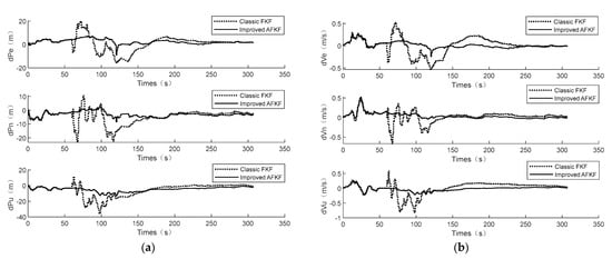
Figure 9.
Comparison of navigation errors between improved AFKF and FKF: (a) Comparison of position errors. (b) Comparison of velocity errors.
5. Conclusions
To address the problem of degraded navigation accuracy caused by GNSS signal blockage in obstructed spaces and insufficient feature points and lighting changes in VNS, this paper proposed an improved AFKF INS/GNSS/VNS integrated navigation algorithm. The algorithm uses INS as the common reference system and constructs sub-filters 1 and 2 by utilizing the position and velocity information of GNSS and the attitude information of VNS as measurement vectors, respectively. A fault detection method combining the proposed residual chi-square test and sliding-window average technique was employed to effectively avoid false alarms and missed detections, thereby improving the fault tolerance of the integrated navigation system. An adaptive information sharing factor was proposed to adaptively allocate the information contribution of each sub-filter according to their respective state covariance matrices, which enhanced the positioning accuracy of the integrated navigation algorithm. Finally, simulations were conducted to evaluate the performance of the improved AFKF algorithm in the presence of obstructed GNSS signals and disturbances affecting the VNS and GNSS sensors separately. Two scenarios were considered where the level of interference varied for the GNSS signals. In both scenarios, the improved AFKF algorithm demonstrated a significant reduction in the position and velocity errors compared to the classic FKF algorithm. Although the improved AFKF algorithm had increased computational requirements, it still met the real-time navigation requirements for unmanned ground vehicles operating in obstructed environments. To further validate the effectiveness of the algorithm, we also conducted simulation experiments on the Gazebo platform. The results of this study are of significance for the practical implementation of navigation systems in obstructed environments.
Author Contributions
All named authors initially contributed a significant part to the paper. Conceptualization, X.W. and Z.S.; methodology, X.W.; software, X.W.; validation, X.W. and L.L.; formal analysis, X.W.; investigation, X.W. and Z.B.; resources, X.W. and L.L.; data curation, X.W. and X.W.; writing—original draft preparation, X.W.; writing—review and editing, X.W.; visualization, X.W.; supervision, Z.S.; project administration, Z.S.; funding acquisition, X.W. All authors have read and agreed to the published version of the manuscript.
Funding
This research was funded by the National Key R&D Program of China (grant no. 2020YFC1511702, 2022YFF0607400), the National Natural Science Foundation of China (61971048), the Beijing Science and Technology Project (Z221100005222024), the Beijing Scholars Program, and the Key Laboratory of Modern Measurement & Control Technology, Ministry of Education.
Institutional Review Board Statement
Not applicable.
Informed Consent Statement
Not applicable.
Data Availability Statement
This study was based on the open-source PSINS toolbox to simulate the navigation data of unmanned vehicles. The open-source PSINS toolkit can be found here: http://www.psins.org.cn/kydm (Version: psins220808). Code and data in the paper can be found here: https://github.com/Wuxj2077/Improved-AFKF (accessed on 5 May 2023).
Conflicts of Interest
The authors declare no conflict of interest.
Abbreviations
The following abbreviations are used in this manuscript.
| INS | Inertial navigation system |
| GNSS | Global navigation satellite system |
| VNS | Visual navigation system |
| Pos | Position |
| Vel | Velocity |
| MAE | Mean absolute error |
| RMSE | Root mean square error |
| FKF | Federated Kalman filter |
| ISF | Information sharing factor |
| IMM | Interacting multiple model |
| RAFUKF | Robust adaptive federal unscented Kalman filter |
| UKF | Unscented Kalman filter |
| SSCST | Simplified state chi-square test |
| IAFKF | Improved adaptive federated filtering |
| E-N-U | East–north–up coordinate system |
| dPe | The position error in the east direction |
| dPn | The position error in the north direction |
| dPu | The position error in the up direction |
| dVe | The velocity error in the east direction |
| dVn | The velocity error in the north direction |
| dVu | The velocity error in the up direction |
| Rmse-P | Root mean square error of position |
| Rmse-V | Root mean square error of velocity |
| ROS | Robot operating system |
References
- Chang, L.; Li, J.; Chen, S. Initial Alignment by Attitude Estimation for Strapdown Inertial Navigation Systems. IEEE Trans. Instrum. Meas. 2015, 64, 784–794. [Google Scholar] [CrossRef]
- Li, K.; Lu, X.; Li, W. Nonlinear Error Model Based on Quaternion for the INS: Analysis and Comparison. IEEE Trans. Veh. Technol. 2021, 70, 263–272. [Google Scholar] [CrossRef]
- Zhu, T.; Liu, Y.; Li, W.; Li, K. The Quaternion-Based Attitude Error for the Nonlinear Error Model of the INS. IEEE Sens. J. 2021, 21, 25782–25795. [Google Scholar] [CrossRef]
- Hu, G.; Gao, B.; Zhong, Y.; Gu, C. Unscented Kalman Filter with Process Noise Covariance Estimation for Vehicular Ins/Gps Integration System. Inf. Fusion 2020, 64, 194–204. [Google Scholar] [CrossRef]
- Shang, X.; Sun, F.; Liu, B.; Zhang, L.; Cui, J. GNSS Spoofing Mitigation With a Multicorrelator Estimator in the Tightly Coupled INS/GNSS Integration. IEEE Trans. Instrum. Meas. 2023, 72, 1–12. [Google Scholar] [CrossRef]
- Chen, L.; Liu, Z.; Fang, J. A Novel Hybrid Observation Prediction Methodology for Bridging GNSS Outages in INS/GNSS Systems. J. Navig. 2022, 75, 1206–1225. [Google Scholar] [CrossRef]
- Gong, X.; Zhang, J.; Fang, J. A Modified Nonlinear Two-Filter Smoothing for High-Precision Airborne Integrated GPS and Inertial Navigation. IEEE Trans. Instrum. Meas. 2015, 64, 3315–3322. [Google Scholar] [CrossRef]
- Zhang, Y.; Yu, F.; Wang, Y.; Wang, K. A Robust SINS/VO Integrated Navigation Algorithm Based on RHCKF for Unmanned Ground Vehicles. IEEE Access 2018, 6, 56828–56838. [Google Scholar] [CrossRef]
- Huang, L.; Song, J.; Zhang, C.; Cai, G. Design and Performance Analysis of Landmark-Based INS/Vision Navigation System for UAV. Optik 2018, 172, 484–493. [Google Scholar] [CrossRef]
- Corke, P.; Lobo, J.; Dias, J. An Introduction to Inertial and Visual Sensing an Introduction to Inertial and Visual Sensing. Int. J. Robot. Res. 2007, 26, 519–535. [Google Scholar] [CrossRef]
- Wang, L.; Li, S. Enhanced Multi-Sensor Data Fusion Methodology Based on Multiple Model Estimation for Integrated Navigation System. Int. J. Control Autom. Syst. 2018, 16, 295–305. [Google Scholar] [CrossRef]
- Zhang, Y.; Dang, Y.; Li, N.; Huang, Y. A Integrated Navigation Algorithm Based on Distributed Kalman Filter. In Proceedings of the 2015 IEEE International Conference on Information and Automation, Lijiang, China, 8–10 August 2015; IEEE: Piscataway, NJ, USA, 2015; pp. 2132–2135. [Google Scholar] [CrossRef]
- Ryu, K.; Back, J. Consensus Optimization Approach for Distributed Kalman Filtering: Performance Recovery of Centralized Filtering. Automatica 2023, 149, 110843. [Google Scholar] [CrossRef]
- Carlson, N.A. Federated Filter for Computer-Efficient, near-Optimal GPS Integration. In Proceedings of the Position, Location and Navigation Symposium—PLANS’96, Atlanta, GA, USA, 22–25 April 1996; IEEE: Piscataway, NJ, USA, 1996; pp. 306–314. [Google Scholar] [CrossRef]
- Carlson, N.A. Federated Square Root Filter for Decentralized Parallel Processors. IEEE Trans. Aerosp. Electron. Syst. 1990, 26, 517–525. [Google Scholar] [CrossRef]
- Yang, Y.; Liu, X.; Zhang, W.; Liu, X.; Guo, Y. A Nonlinear Double Model for Multisensor-Integrated Navigation Using the Federated EKF Algorithm for Small UAVs. Sensors 2020, 20, 2974. [Google Scholar] [CrossRef]
- Wang, Y.; Zhao, B.; Zhang, W.; Li, K. Simulation Experiment and Analysis of GNSS/INS/LEO/5G Integrated Navigation Based on Federated Filtering Algorithm. Sensors 2022, 22, 550. [Google Scholar] [CrossRef] [PubMed]
- Jiang, R.; Li, J.; Xu, Y.; Wang, X.; Li, D. Fault-tolerant GPS-AOA-SINS integrated navigation algorithm based on federated Kalman filter. J. Commun. 2022, 43, 78–89. [Google Scholar]
- Zhang, H.; Zhang, H.; Xu, G.; Liu, H.; Liu, X. Attitude832 Anti-Interference Federal Filtering Algorithm for MEMS-833 SINS/GPS/Magnetometer/SV Integrated Navigation System. Meas. Control. 2020, 53, 46–60. [Google Scholar] [CrossRef]
- LV, J.X.; ZHOU, Z.H.; Fu, J.J. Application of Adaptive Federated Kalman Filter in Robot Integrated Navigation System. Meas. Control. Technol. 2017, 36, 15–19. [Google Scholar]
- Xu, J.; Xiong, Z.; Liu, J.; Wang, R. A Dynamic Vector-Formed Information Sharing Algorithm Based on Two-State Chi Square Detection in an Adaptive Federated Filter. J. Navig. 2019, 72, 101–120. [Google Scholar] [CrossRef]
- Zhai, C.; Wang, M.; Yang, Y.; Shen, K. Robust Vision-Aided Inertial Navigation System for Protection Against Ego-Motion Uncertainty of Unmanned Ground Vehicle. IEEE Trans. Ind. Electron. 2021, 68, 12462–12471. [Google Scholar] [CrossRef]
- Shen, K.; Wang, M.; Fu, M.; Yang, Y.; Yin, Z. Observability Analysis and Adaptive Information Fusion for Integrated Navigation of Unmanned Ground Vehicles. IEEE Trans. Ind. Electron. 2020, 67, 7659–7668. [Google Scholar] [CrossRef]
- Lyu, W.; Cheng, X.; Wang, J. Adaptive Federated IMM Filter for AUV Integrated Navigation Systems. Sensors 2020, 20, 6806. [Google Scholar] [CrossRef] [PubMed]
- Lyu, X.; Hu, B.; Wang, Z.; Gao, D.; Li, K.; Chang, L. A SINS/GNSS/VDM Integrated Navigation Fault-Tolerant Mechanism Based on Adaptive Information Sharing Factor. IEEE Trans. Instrum. Meas. 2022, 71, 1–13. [Google Scholar] [CrossRef]
- Dai, J.; Hao, X.; Liu, S.; Ren, Z. Research on UAV Robust Adaptive Positioning Algorithm Based on IMU/GNSS/VO in Complex Scenes. Sensors 2022, 22, 2832. [Google Scholar] [CrossRef]
- Chen, S.; Wang, N.; Chen, T.; Yang, Y.; Tian, J. Confidence test adaptive federated Kalman filtering and its application in combined navigation of underwater robots. Chin. J. Ship Res. 2022, 17, 203–211+220. [Google Scholar] [CrossRef]
- Xiong, H.; Bian, R.; Li, Y.; Du, Z.; Mai, Z. Fault-Tolerant GNSS/SINS/DVL/CNS Integrated Navigation and Positioning Mechanism Based on Adaptive Information Sharing Factors. IEEE Syst. J. 2020, 14, 3744–3754. [Google Scholar] [CrossRef]
- Shen, K.; Xia, Y.; Wang, M.; Neusypin, K.A.; Proletarsky, A.V. Quantifying Observability and Analysis in Integrated Navigation. Navig. J. Inst. Navig. 2018, 65, 169–181. [Google Scholar] [CrossRef]
- Jian-wei, G.; Wei, X.U.; Yan, J.; Kai, L.I.U.; Hong-fen, G.U.O.; Yin-jian, S.U.N. Multi-Constrained Model Predictive Control for Autonomous Ground Vehicle Trajectory Tracking. J. Beijing Inst. Technol. 2015, 24, 441–448. [Google Scholar] [CrossRef]
Disclaimer/Publisher’s Note: The statements, opinions and data contained in all publications are solely those of the individual author(s) and contributor(s) and not of MDPI and/or the editor(s). MDPI and/or the editor(s) disclaim responsibility for any injury to people or property resulting from any ideas, methods, instructions or products referred to in the content. |
© 2023 by the authors. Licensee MDPI, Basel, Switzerland. This article is an open access article distributed under the terms and conditions of the Creative Commons Attribution (CC BY) license (https://creativecommons.org/licenses/by/4.0/).