Abstract
Structural health monitoring systems continuously monitor the operational state of structures, generating a large amount of monitoring data during the process. The structural responses of extreme events, such as earthquakes, ship collisions, or typhoons, could be captured and further analyzed. However, it is challenging to identify these extreme events due to the interference of faulty data. Real-world monitoring systems suffer from frequent misidentification and false alarms. Unfortunately, it is difficult to improve the system’s built-in algorithms, especially the deep neural networks, partly because the current neural networks only output results and do not provide an interpretable decision-making basis. In this study, a deep learning-based method with visual interpretability is proposed to identify seismic data under sensor faults interference. The transfer learning technique is employed to learn the features of seismic data and faulty data with efficiency. A post hoc interpretation algorithm, termed Gradient-weighted Class Activation Mapping (Grad-CAM), is embedded into the neural networks to uncover the interest regions that support the output decision. The in situ seismic responses of a cable-stayed long-span bridge are used for method verification. The results show that the proposed method can effectively identify seismic data mixed with various types of faulty data while providing good interpretability.
1. Introduction
Data acquisition is a prerequisite for structural health monitoring (SHM). Various sensing techniques have been researched and applied [1,2,3]. However, the massive amount of monitoring data are contaminated by multiple types of anomalies, which could negatively affect the expected system functionality [4]. While pursuing the goal of extreme event identification, such as identifying earthquakes timely to ensure structural safety, the real seismic response could be misclassified as anomalies caused by sensor faults, or vice versa. Therefore, these anomalies must be taken into consideration in real-world applications.
A sensor fault can be defined as an unexpected deviation in the observed signal output without any malfunction in the system [5]. Bao et al. [6] first combined computer vision and deep learning to diagnose anomalies by utilizing time-domain images transformed from SHM data. Later, Tang et al. [7] further improved this method using stacked time-frequency grayscale maps and a convolutional neural network for identifying anomalies, achieving higher accuracy. Saeed et al. [8] used an Extremely Randomized Tree to generate a decision function, where anomaly patterns were identified based on the number of votes received from each tree in the forest-like structure. Smarsly and Law [9] proposed an analytic redundancy approach that embeds neural networks into individual sensors of the SHM system, each of which can autonomously detect and isolate sensor faults. Jan et al. [10] proposed a distributed sensor-fault detection and diagnosis system, which transmits sensed data periodically to a distant node and obtains a quick decision about the presence of a fault. Li et al. [11] obtained cable tension data by utilizing source separation during the pre-processing stage to eliminate the effects of sensor faults. Mao et al. [12] combined the generative adversarial networks with an unsupervised learning method to achieve sensor anomaly detection through a computer vision approach, which also addresses the issue of class imbalance in anomalous data. It is worth noting that the aforementioned methods have achieved good accuracy in anomaly detection, but they mainly focus on detecting sensor faults and ignore that extreme events can produce similar anomalous data, which should be given special attention.
In practical engineering, the extreme events data detected by the SHM system is often mixed with anomaly data caused by sensor faults. It is a challenge to distinguish the two in massive data. Researchers have been working to enable SHM systems to identify various types of extreme events in recent years. Sun et al. [13] analyzed the impact of a ship collision on the bridge using SHM data, GPS measurements were utilized to determine modal parameters and assess the bridge’s status. Zhang et al. [14] used Kernel Density Estimation (KDE) method to identify bridge waterways, then applied Velocity Obstacle (VO) method to detect potential ship collisions. Lim et al. [15] proposed a typhoon detection method based on long short-term memory (LSTM) network, which can predict the wind speed of the bridge using the time-shift data correction (TSDC) method. In seismic monitoring, Gentili et al. [16] used an artificial neural network approach to detect seismic s-wave and p-wave onset times, which has more robustness compared to traditional manual identification methods. Perol et al. [17] developed ConvNetQuake, a CNN for seismic detection and location from a single waveform, achieving faster detection speed than established methods. Ross et al. [18] used the vast manually labeled data archives of the Southern California Seismic Network to train a CNN seismic wave phases detection and achieved sensitive and robust performance. Zhang et al. [19] utilized unsupervised learning techniques in conjunction with support vector data description for anomaly detection. Extreme events are successfully separated as a special pattern from normal, anomalous, and unknown patterns. At the stage of the post assessment of earthquakes, Barkhordari et al. proposed ensemble models [20] and a hybrid wavelet scattering network-based model [21] to identify damage in reinforced concrete structures after earthquakes, demonstrating higher accuracy compared to single models.
Although the aforementioned anomaly detection methods have demonstrated adequate performance in various scenarios, two common issues exist: Firstly, most of the method’s process either sensor faults (as anomalies) or extreme events (as anomalies). The concurrence of two types of data is hardly considered. Secondly, these algorithms, especially the deep learning-based methods, only output results as black-boxes, leading to insufficient trust in their decisions.
To open the black-boxes of deep neural networks (DNN), interpretation algorithms for deep models have been researched in recent years. Overall, DNN’s interpretability is categorized into pre-hoc and post hoc interpretability, with the cut-off point being the completion of the network’s training. The research subject of pre-hoc interpretability is neural network models, and it focuses on understanding the inner mechanism of the model architecture; post hoc interpretability has developed as a subfield of machine learning (ML) that seeks to augment the learned representations and the decisions with human-interpretable explanations [22]. Xu et al. [23] input the perturbations into the sample so that the prediction result can represent the importance of each location in the image. Selvaraju et al. [24] employed gradient information in the neural network’s backpropagation to show the depth model’s concentration on areas of the image. Dosovitskiy et al. [25] used an up-convolutional network to visualize CNNs. As for the application of the interpretability algorithm, Harsh et al. [26] used a DNN combining the Grad-CAM algorithm to detect COVID-19, and the diagnosis was indicated by showing the patient’s symptoms. Xiao et al. [27] used FCSNet to detect surface scratch defects and embedded Grad-CAM algorithm to visualize its interest region.
To further the research on the two aforementioned problems, we proposed a deep learning approach capable of effectively identifying seismic responses amidst faulty data interference, while also providing trustworthy visual interpretability. The main innovations of this article are as follows:
- (a)
- The seismic responses of a cable-stayed long-span bridge are successfully identified under the interference of the multi-class monitoring system’s faulty data.
- (b)
- Transfer learning technique is utilized for efficient learning of monitoring data, especially the small-sample patterns.
- (c)
- An interpretation algorithm, termed Grad-CAM, is embedded into the DNN, enabling the model to provide interpretable visual evidence while outputting classification results.
2. Methods
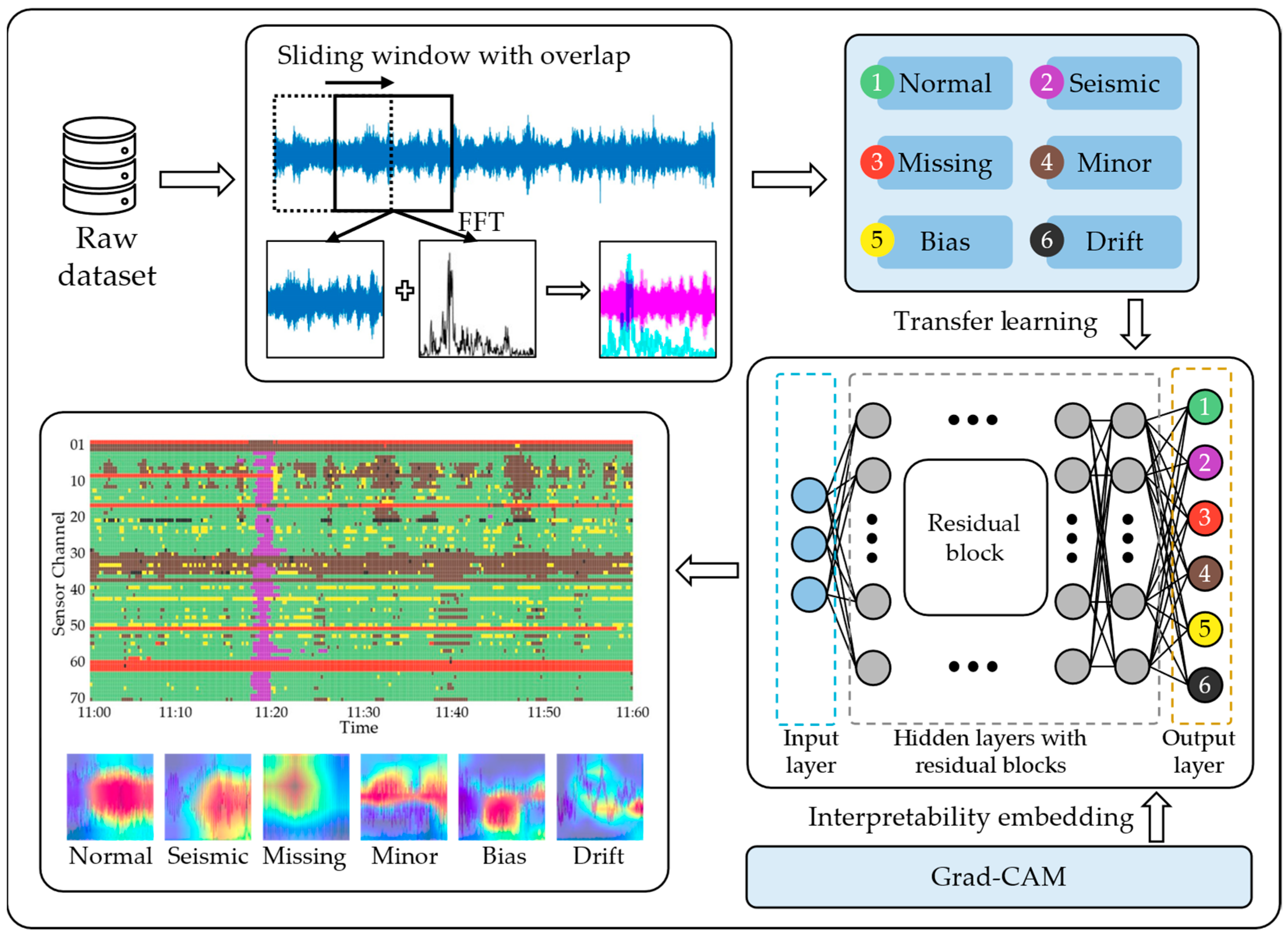
The framework of the vision-based trustworthy anomaly detection method is shown in Figure 1. In the first step, a real-world monitoring dataset, which consisted of four types of anomalies and seismic response data, was collected from a long-span cable-stayed bridge. Then, the acceleration data were piecewise transformed into forming the dual channel time-frequency (T-F) images. Meanwhile, these T-F images were manually labeled into six classes according to their features and the groundtruth. Transfer learning was then utilized for efficient learning. T-F images were used to fine-tune the ResNet34, which was trained previously for daily-life image classification. The fine-tuned network was able to learn features of various anomalies with higher efficiency compared to training a random-initialized neural network from scratch. Additionally, Grad-CAM was integrated into the well-trained deep ResNet34, enabling the neural network to provide the region of interest while outputting the classification results.
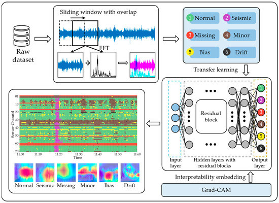
Figure 1.
Framework of the proposed method.
2.1. Data Representation Space
Monitoring data can be input into a neural network in multiple representation spaces. Zhang et al. [28] considered a vibration time series as a one-dimensional vector, which was input into a CNN for structural status identification. Mao et al. [10] transformed the time series data into Gramian Angular Field (GAF) images and implemented computer vision methods to detect anomalous data. Yang et al. [29] used video frames from a camera as the input to capture the structural modes, wherein the same effect as the sensor’s vibration time series has been achieved with higher efficiency. Canizo et al. [30] proposed a multi-time series anomaly detection method, which employed independent CNNs to detect anomalies in each sensor; it used multiple one-dimensional time series as inputs to each CNN, avoiding the influence of sensors with different natures. In this paper, we followed the vision-based anomaly detection method [7] to present the monitoring data. Specifically, the continuous time series were segmented by a sliding window with an overlap, then plotted in the time and frequency domains, respectively. A dual channel time-frequency image (T-F image) was made by simply stacking a pair of time- and frequency-response. Different from other image space-based representation methods, the vision-based method keeps comprehensible visual features, which aligns with the human experience. Therefore, the monitoring data were presented by dual channel time-frequency images considering the verified representation ability and intuitive interpretability.
2.2. ResNet34 as the Feature Extractor
Deep neural networks can extract rich image features in classification tasks by increasing the number of layers. In fact, in the ImageNet classification task, a deep model with a depth of sixteen has exceeded human recognition accuracy [31], demonstrating the impact of network depth on feature extraction ability. However, as the network layers become deeper, the problem of gradient vanishing and gradient explosion arise during the training process, leading to difficulty in achieving convergence of training results [32]. Gradient vanishing/exploding occurs during backpropagation while training neural networks and may grow significantly as the network’s depth increases [33]. Moreover, batch normalization and weight regularization have substantially fixed this issue, but the above methods do not solve the problem of decrease in accuracy that occurs with the increase in the model depth, also known as the degradation problem [34].
2.2.1. ResNet34 Architecture
The degradation problem manifests as the decreased performance of deep neural networks compared to their shallower counterparts. Suppose that a deep neural network reaches its optimal state at a certain depth, in that case, the extra layers beyond that point can be replaced by identity mapping connections, meaning the extra layers are bypassed during computation. In theory, this method can solve the degradation problem, making the deep neural network perform as well as its corresponding shallower counterpart. However, traditional nonlinear representations of multilayer network structures are difficult to represent identity mapping. Inspired by identity mapping, He proposed a deep residual learning framework to solve the degradation problem [34].
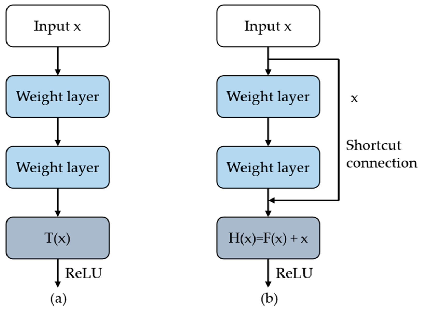
Figure 2 shows the difference in the operation process between residual networks and traditional networks, also called plain networks. Residual networks possess an additional shortcut connection structure compared to plain networks. In plain networks, as shown in Figure 2a, we denote the underlying mapping to be fit by a few stacked weight layers as T(x), where x is the output value of the previous block. However, the computed T(x) cannot remain constant and equal to x, leading to the degradation phenomenon. In contrast, residual networks, as shown in Figure 2b, modify the underlying mapping to H(x), and the stacked layers are assigned to learn a residual mapping: F(x) = H(x) − x, allowing the network to have two paths during forward propagation, namely F(x) and x, which can also be viewed as parallel circuits. When the network reaches the optimal number of layers, the identity mapping can be realized by setting F(x) to zero when passing through the extra weight layers, so that its underlying mapping can be written as H(x) = x.
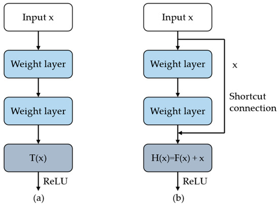
Figure 2.
(a) A building block of a plain network; (b) A building block of a residual network.
He [34] demonstrated the performance of residual and plain net with the same number of layers and the same hyperparameters for the image classification tasks. Experimental results showed that the network with residual mapping has higher accuracy in the test of ImageNet. He further designed ResNet with different depth layers (18, 34, 50, 101, and 152) to address more complex classification tasks [34]. In this paper, to balance the number of training sets and accuracy, ResNet34 was chosen as the feature extractor. The structure of ResNet34 is shown in Figure 3. ResNet34 is composed of a convolutional layer, four residual blocks, and a fully connected layer, where each residual block represents a conventional feed-forward network with shortcut connections.

Figure 3.
The network architecture of ResNet34.
2.2.2. Transfer Learning
Transfer learning (TL) is a machine learning technique that focuses on transferring knowledge across domains [35]. Training a deep model from scratch requires a large training set and a significant amount of time, but the training results are not always guaranteed to converge. TL can address these issues. Pan and Yang [36] suggested that having a training task in one area of interest and enough training data in another area of interest, TL could be employed to reduce expensive data labeling efforts while improving learning performance. Motivated by transfer learning, Xu [37] proposed a nested attribute-based few-shot meta learning paradigm for structural damage identification, which achieved better results than traditional supervised learning with limited training samples. Lin [38] defined transfer learning as follows: Given a source domain and learning task , and a target domain and learning task , TL aims to enhance the learning performance of the target predictive function in by utilizing knowledge from and , where ≠ , or ≠ .
Fine-tuning is a subcategory of transfer learning, which involves modifying the weights of some layers in a pre-trained neural network and uses these weight layers to train another model on target data [39]. Typically, the early layers of a CNN learn to recognize low-level visual features that are applicable to most image classification tasks. In contrast, the last few layers of the CNN are responsible for identifying high-level visual features. Fine-tuning generally refers to the modification of the last few layers [40]. This technique can prevent performance degradation and accelerate network convergence. In this study, we employ fine-tuning during the training process for anomaly detection, utilizing a pre-trained ResNet34 model trained on ImageNet as the base network.
2.3. Grad-CAM
Gradient-weighted Class Activation Mapping (Grad-CAM) is a CNN-based technique that generates visual explanations for decisions [24]. It reflects the deep model’s interest region using back propagation gradient information from the neural network’s feature maps, and the interest region is represented by a heat map.
Note that Grad-CAM is a modified form of the Class Activation Mapping (CAM) algorithm. The CAM algorithm replaces the fully connected layer in CNNs with the global average pooling layer (GAP) to generate interpretable output [41]. The GAP computes the average value of each feature map in the last convolutional layer of the CNN, with each value representing the importance of the corresponding feature map to the predicted class, denoted by , where is the feature map number for a target class . Next, the feature layers are weighted by their corresponding importance weight , and then stacked altogether to form a matrix. This matrix is then up-sampled to the size of the input image to generate the class activation map. The mathematical representation of CAM is as follows:
where, denotes the activation of feature layer in a certain layer of the CNN at a spatial location , and denotes the weight related to the class for the feature map .
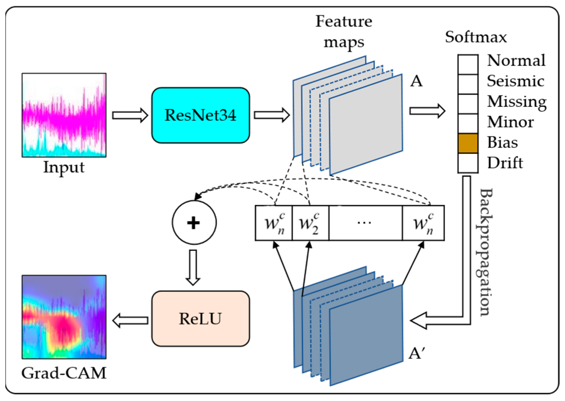
Although the CAM algorithm can demonstrate the interest region of the deep model’s decision, it has to replace the fully connected layer with a GAP layer, which alters the network’s structure and may decrease its performance. Furthermore, it is necessary to retrain the network, which is time-consuming. In this regard, Selvaraju et al. [24] proposed the Grad-CAM method. Grad-CAM directly uses the gradient information as important weights to generate the activation map without any change or modification for the network structure. Therefore, Grad-CAM achieves better universality and convenience compared with CAM. The workflow of the Grad-CAM algorithm is shown in Figure 4.
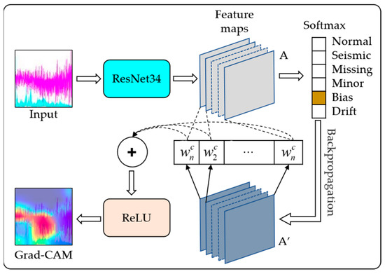
Figure 4.
Flowchart of Gradient-weighted Class Activation Mapping.
It is suggested that feature maps maintain the class-specific information in the image, and the feature maps of deeper convolutional layers preserve richer semantic information but a lower degree of granularity [24]. Figure 4 illustrates that the th feature map, denoted as , of a convolutional layer contains semantic information relevant to the object of interest. This information is propagated to the Softmax layer to predict the object category. Then, the gradient of the probability for class c is computed, denoted as , and the element in row i and column j of the matrix can be computed as follows:
where, represents the contribution of each element in to the category , so its mean value for the elements of can reflect the importance of th feature map , as shown in Equation (3). Grad-CAM is subsequently obtained by summing the weighted feature layers, and then passing through the ReLU layer. The mathematical representation is in Equation (4).
where, denotes the total number of elements in a feature map, i.e., . In this paper, the Grad-CAM algorithm is embedded into the ResNet34 for interpretable event and anomaly detection. The interest regions extracted by convolutional layers from shallow to deep can be used to investigate the inner mechanisms of deep models.
3. Example
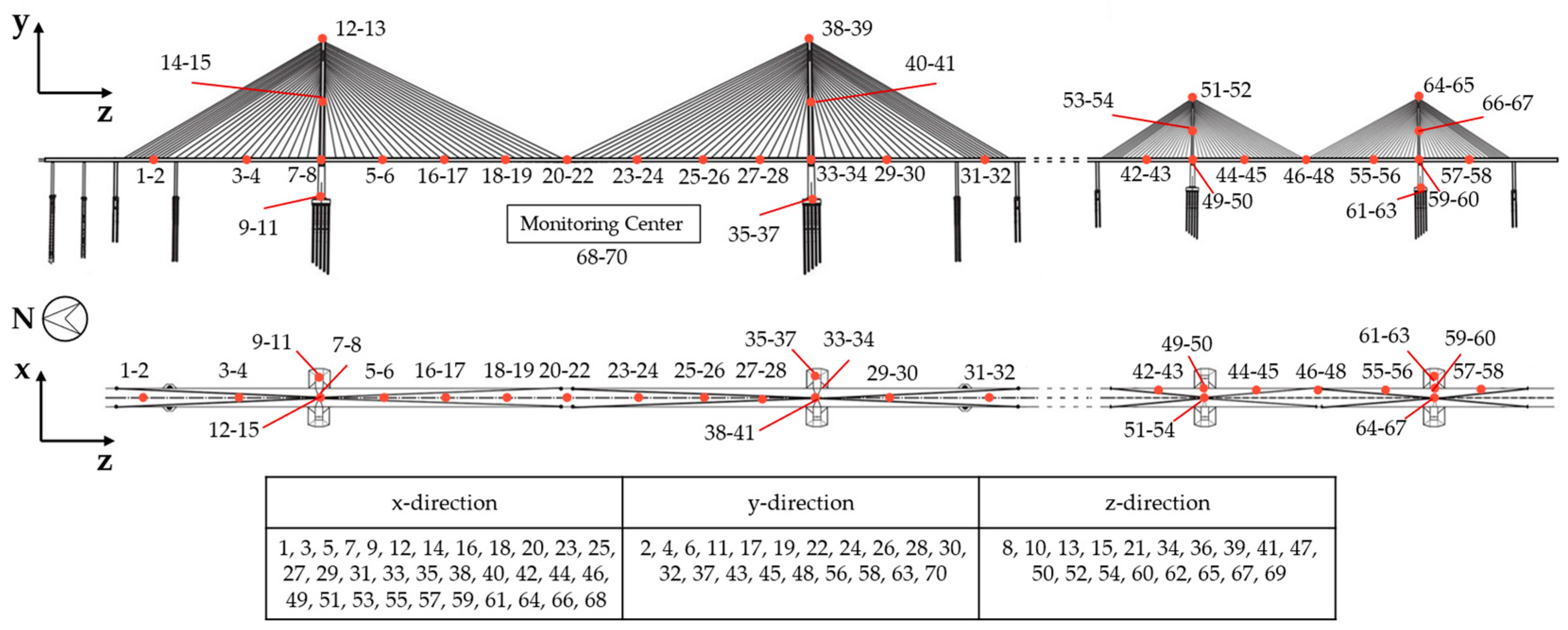
The monitoring data of a long-span cable-stayed bridge, which consists of a northern-branch bridge and a southern-branch bridge, was used for method verification. Specifically, the acceleration data of the bridge’s girders and piers, totaling 70 channels with a sampling frequency of 50 Hz, were employed. The sensor locations and sensing directions are shown in Figure 5.
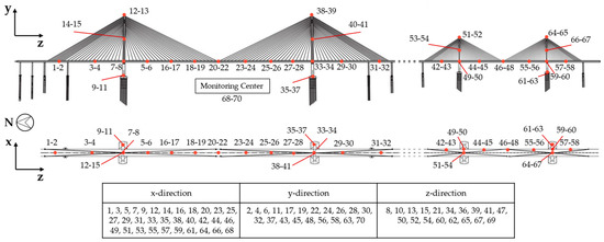
Figure 5.
Sensor locations of the cable-stayed long-span bridge (consists of a northern-branch bridge and a southern-branch bridge).
3.1. Data Collection and Dataset Generation
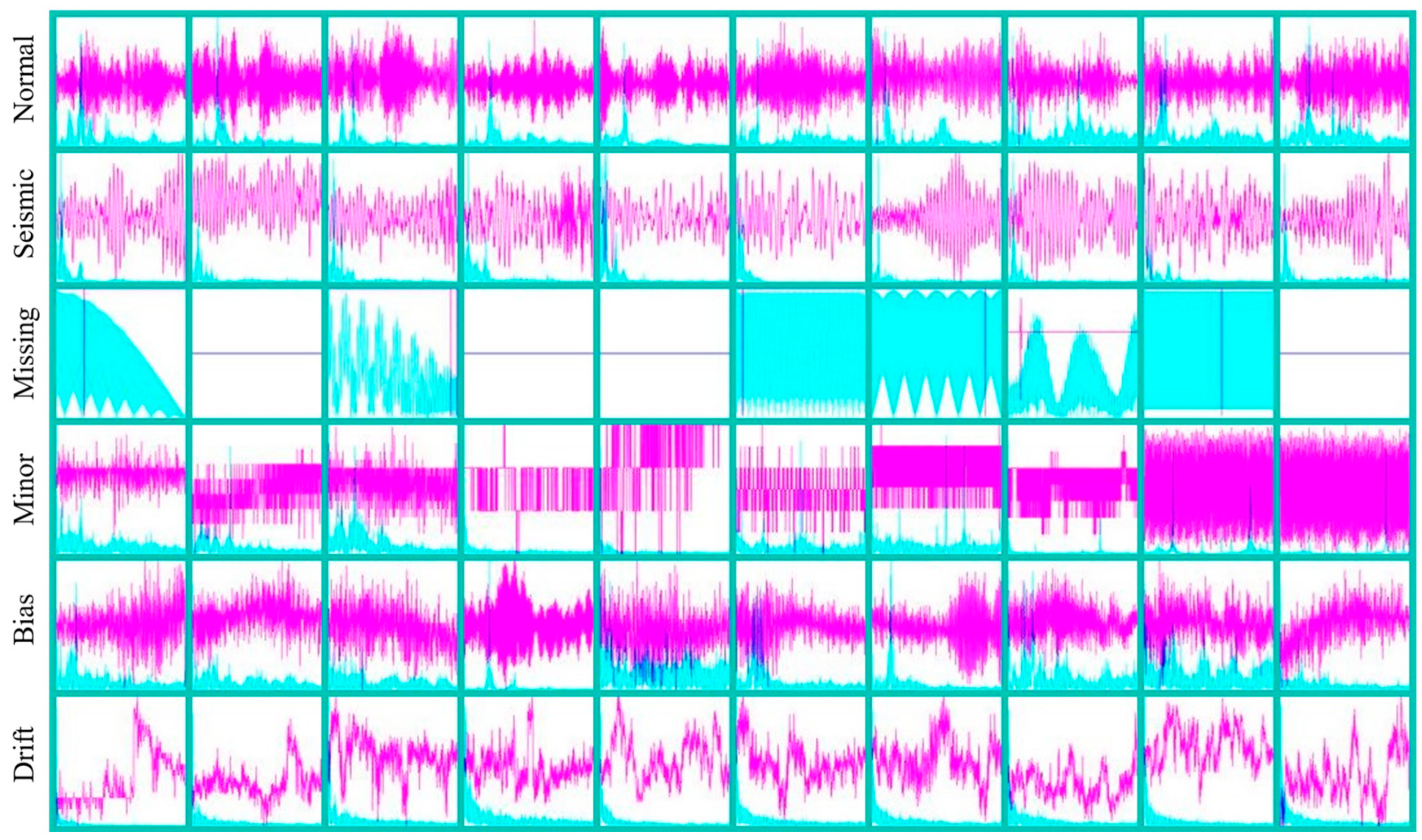
We collected four seismic vibration responses of a long-span cable-stayed bridge in China, as shown in Table 1. Each seismic event was stored in one-hour time series of the monitoring system. In this paper, we follow the vision-based anomaly detection method [7] to generate the image datasets. The continuous time series were segmented by a 30-s sliding window with a 15-s overlap, then plotted in the time and frequency domains. A dual-channel time-frequency image was made by simply stacking a pair of time and frequency responses. The dimension of a T-F image is 100 × 100 × 2. Note that various anomalies exist in the monitoring data due to system malfunctions. Therefore, based on the visual features and the groundtruth, we manually labeled the T-F images according to Table 2 into six classes: Normal, Seismic, Missing, Minor, Bias and Drift. Each pattern of the T-F images is shown in Figure 6. A labeled dataset of 67,200 samples was generated, as shown in Table 3.

Table 1.
The seismic information.

Table 2.
Description of each data pattern.
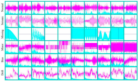
Figure 6.
Examples of normal, seismic, and anomalous patterns.

Table 3.
Number of samples for each type in each event.
It is worth noting that the data labeling in this study does not consider the quantitative values of the vibration acceleration, but only the visual features of the T-F images, so labeling the seismic data mainly relies on the following two aspects: firstly, the seismic information released by the China Earthquake Networks Center is utilized, but due to the seismic propagation, the seismic response of bridges lags behind the occurrence of earthquakes by several seconds; secondly, the seismic response of long-span bridges exhibits long-period characteristic [42].
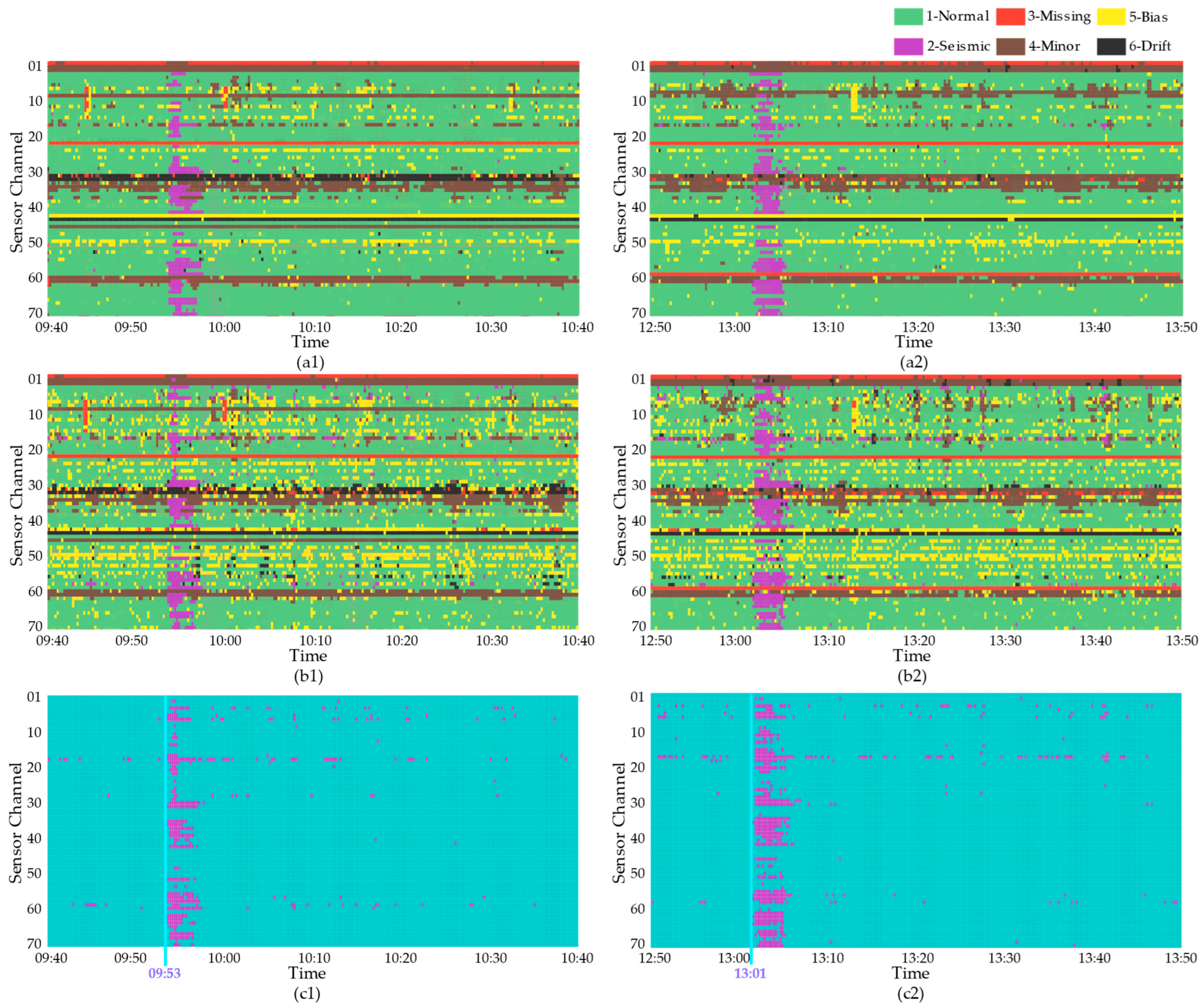
Next, seismic events No. 1 and No. 2 are used for neural network training, and seismic events No. 3 and No. 4 are for testing. The number of samples per class in the balanced training set is set to 1000, and 200 samples from each class are selected as the validation set. Figure 7 shows the distribution of anomalies for seismic events No. 1 and No. 2. The starting time of seismic No.1 was around 11:17:30, while in seismic No. 2, it was around 21:57:15, followed by an aftershock at around 22:12. Note that the vibration acceleration data did not concurrently exhibit the seismic response characteristics, even some of the channels’ data were never labeled as seismic responses from start to end. Some channels with persistent sensor malfunctions failed to record the earthquake, resulting in mostly Missing or Minor data spreading throughout the entire time span. Meanwhile, the pattern Bias was scattered in both temporal and spatial dimensions, which may interfere with the seismic detection.

Figure 7.
Visualization of samples distribution in: (a) seismic event No. 1; (b) seismic event No. 2. The vertical cyan lines indicate the time when the monitoring system detected the earthquake.
3.2. Neural Network Training and Validation
As a classification task, accuracy, precision and recall are used as metrics to evaluate the model’s performance. Accuracy is defined as the ratio of correctly predicted samples to the total number of predicted samples, regardless of their positive or negative status. Precision, on the other hand, is the ratio of true positive samples to the total number of samples predicted as positive for a given class, thus quantifying the proportion of correct positive predictions among all positive predictions made by the model. Recall is defined as the ratio of true positive samples to the total number of actual positive samples for a given class, measuring the proportion of positive samples that the model correctly identified. The mathematical expressions for these metrics are as follows:
where, tp denotes “true positive” (Predict positive classes as positive classes); fp denotes “false positive” (Predict negative classes as positive classes); tn means “true negative” (Predict negative classes as negative classes); and fn means “false negative” (Predict positive classes as negative classes).
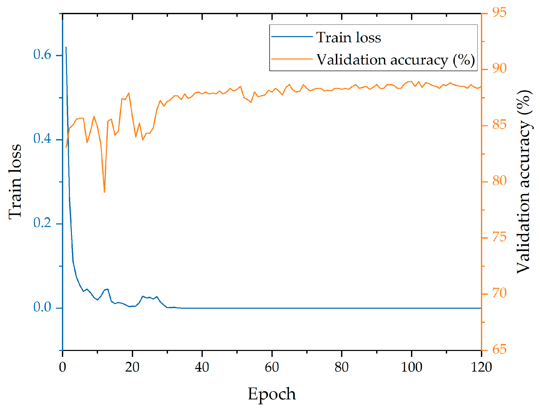
In this study, the neural network’s training was performed on a computer with a CPU of Intel Core i9-11900K and a GPU of NVIDIA A6000. The batch size was set to 50, the learning rate was 0.001, and the number of epochs was 120. The learning rate reduced to half of its previous value after ten epochs for training stability. The model’s performance metrics, i.e., accuracy and loss, on both the training and validation sets of each epoch were reserved. The validation accuracy was used as the criterion for selecting the best-performance model, which occurred at the 98th epoch, as shown in Figure 8.
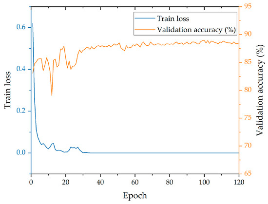
Figure 8.
Train loss and validation accuracy.
The confusion matrix in Figure 9 shows the best-performance model’s classification performance on the validation set. It is shown that the seismic precision and recall rates on the validation set are 91.5% and 92.0%, respectively, which suggests a high probability that the monitoring system correctly detects a real seismic event rather than a false alarm due to sensor faults. Although the deep model has achieved an accuracy of nearly 90% for multi-class anomaly classification, the precision and recall rates for the Bias class are relatively low. We will investigate this further in the next chapter.
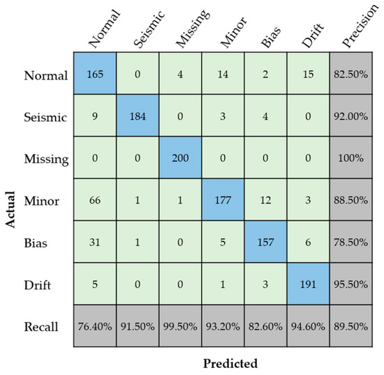
Figure 9.
The confusion matrix on the validation set.
3.3. Test Using Real-World Seismic Events
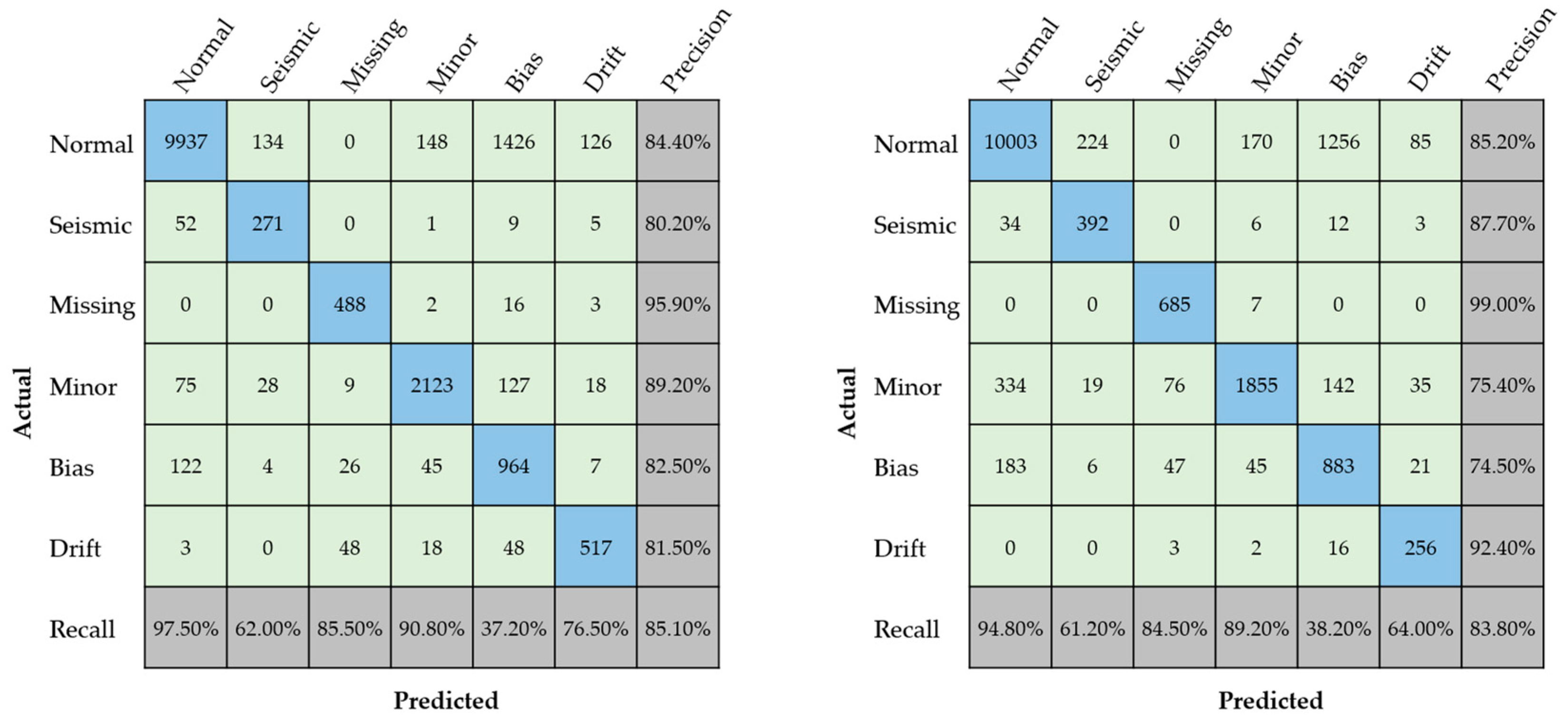
To assess the generalization ability of the chosen model, seismic events No. 3 and No. 4 were utilized for testing. The confusion matrixes of the test results are presented in Figure 10. It is shown that the neural network achieves similar detection performance on the two seismic events, reaching over 83%. Forcing on seismic event No. 3, the pattern Seismic exhibited a precision of 62.0% and a recall of 80.2%. In the predicted results, 134 samples of the pattern Normal were misclassified as Seismic, causing the relatively low precision. Moreover, the pattern Normal had the highest precision of 97.5%, while the “Bias” pattern was less satisfactory, with a precision of 37.7%. This result may be attributed to the model’s inability to properly distinguish between “Normal” and “Bias” or the model’s focus on only one of conditions despite the coexistence of both conditions in a certain time interval.
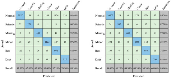
Figure 10.
Confusion matrix of seismic events No. 3 and No. 4.
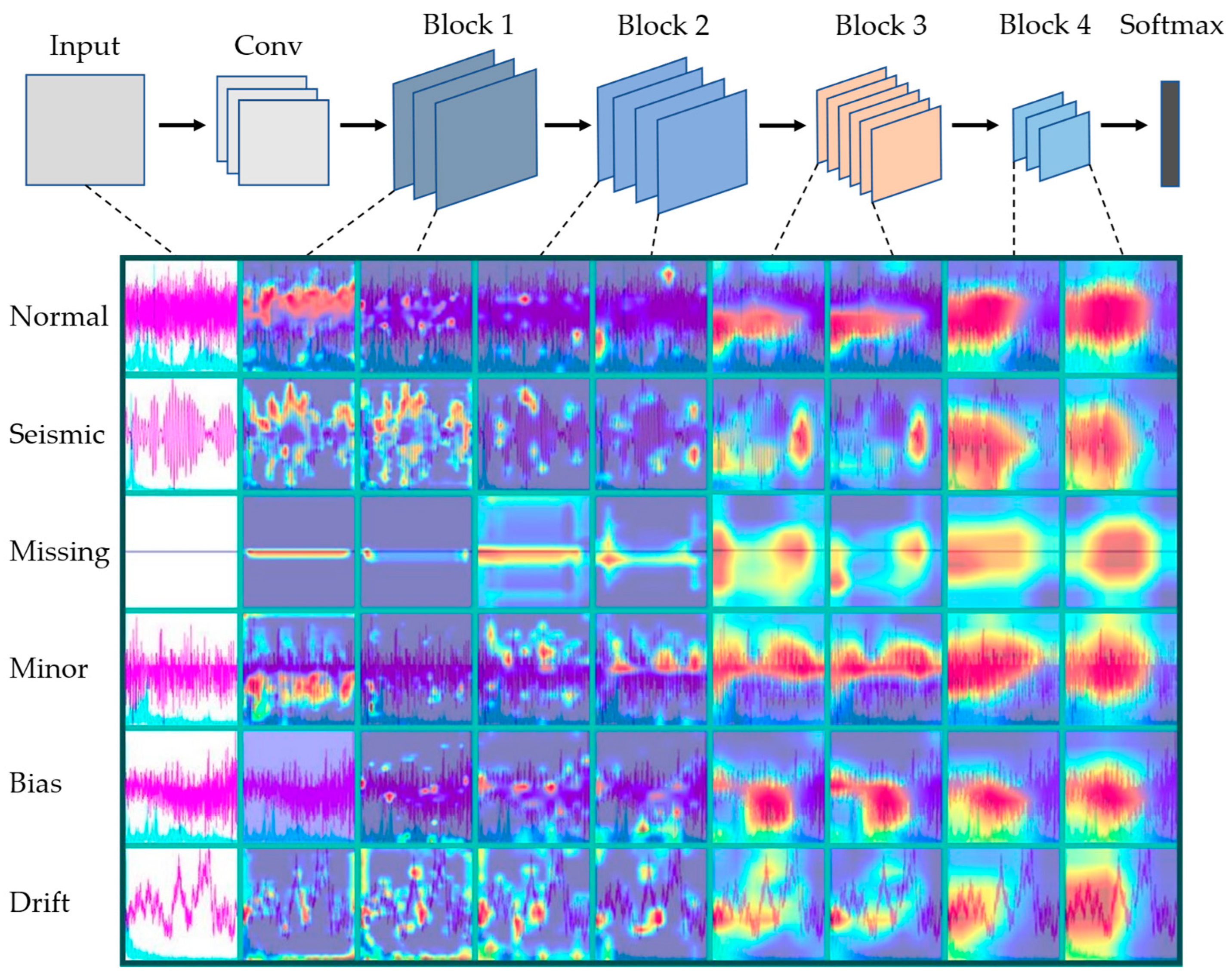
So far, the classification performance has been exhibited and discussed. Classification results were provided without additional comprehensible information. Therefore, an interpretation algorithm for neural networks was employed in this paper to further investigate the classification mechanism. Specifically, the Grad-CAM algorithm was used to visualize the interest region of the correctly classified samples at different depths of neural networks. As shown in Figure 11, the utilized ResNet34 consists of convolutional layers and four residual blocks, apart from the conventional input and output layers. Usually, only the gradient information from the last convolutional layer is used to generate the model’s interest region. In this manuscript, the first and last convolutional layers of each residual block were selected for comprehensive visualization. It is shown that the interest regions in the shallow layers, i.e., Block 1 and Block 2, are relatively scattered, mostly appearing as points or lines. Additionally, both temporal features and frequency-domain features were considered by the neural network. The visual explanations denote that the shallow layers of the neural network mainly extracted low-level features. Meanwhile, it can be observed that the interest region in layers of Block 3 and Block 4 converge to form a continuous focusing surface, which is highly similar to the way human eyes focus on images. The globally most representative features in the images are captured. Further, Block 4 has a broader area of interest than Block 3; the reason for this phenomenon is that the deeper the convolutional layer, the smaller the image size, so the range of the interest region relatively expanded. By visualizing the interest regions of neural networks, this approach reveals the local and global features for each sample’s classification, helping human users understand the decision basis of neural networks and enhancing trust in their decision-making process.

Figure 11.
The interest regions of the images that residual blocks in ResNet34 focus on.
4. Discussions
4.1. Panorama of Data Distribution
Next, the spatial and temporal distribution of the detection results for the seismic event No. 3 and No. 4 are provided and compared with the manual labels’. As shown in Figure 12, the upper plot represents the manually labeled distribution, and the middle plot represents the neural network’s detection results. Additionally, the lower plot specifically shows the distribution of detected seismic data among other classes. For seismic event No. 3, it is shown that the starting time of the bridge’s seismic response was around 9:53:15, consistent with the groundtruth, but delayed by less than one minute compared to the earthquake occurrence time at the epicenter. Similar to seismic events No. 1 and No. 2, not all channels’ vibration data exhibited seismic response characteristics during the events, such as Channel 2, 3, 10, and 36, shown in Figure 12a1. Due to the interference of sensor malfunctions, some channels failed to record the seismic event. For example, the pattern Missing spread throughout the entire time span in channel 2 and channel 24. Meanwhile, the pattern Bias was scattered in both temporal and spatial dimensions, which interfered with the seismic detection. Similar results were obtained in the detection of seismic event No. 4. It is noteworthy that in the detection results of seismic event No. 4, the starting times of the detected seismic event in most channels were consistent, whereas manually labeled data in Figure 12a2 exhibited varied time difference across different channels.
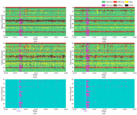
Figure 12.
Comparison of the data distribution for seismic event No. 3 (left) and No. 4 (right): (a1,a2) actual data anomaly distribution, (b1,b2) detection results, and (c1,c2) seismic distribution in the detection results.
4.2. Misclassification Cases
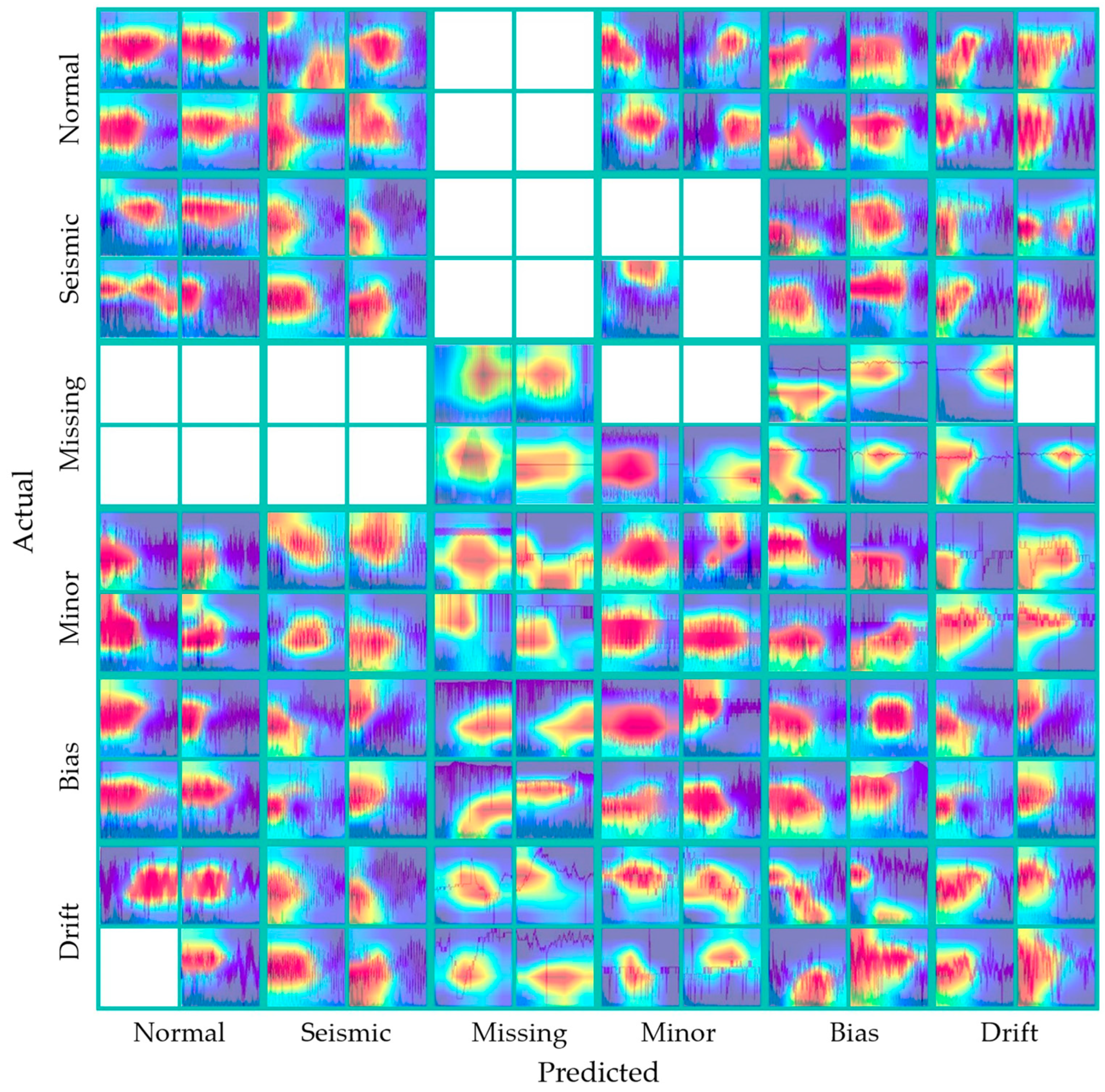
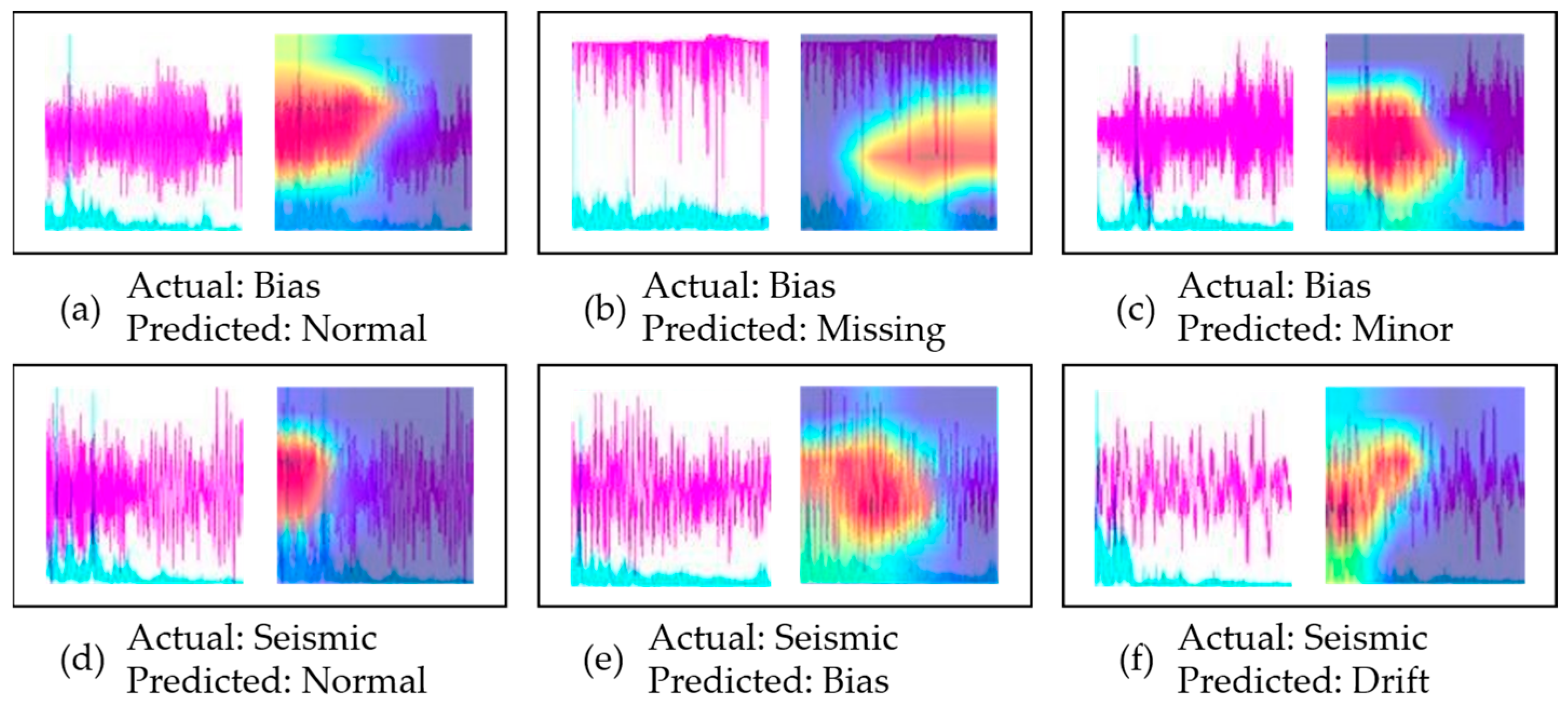
To further investigate the classification results, some classified examples arranged in a confusion matrix of seismic event No. 3 are provided in Figure 13. Additionally, corresponding heat map interpretations from the ResNet34’s Block 3 are demonstrated in Figure 14. A relatively clear phenomenon is that the neural network tends to focus on the first half of the time series, regardless of whether the sample is correctly classified. Specifically, Figure 15 displays six typical misclassified samples. In Figure 15a, we can see that the pattern Bias was misclassified as Normal. This is because the neural network focuses on the first half of the time history, which does conform to the characteristics of the pattern Normal, while the latter half of the time history was neglected. In Figure 15b, the time history exhibits strong bias characteristics. Unfortunately, the neural network empirically paid attention to the vertically central region of the image, and therefore misclassifying the sample as the pattern Missing due to the blank area. It should be clarified that the number of such samples in the training set is limited, so the neural network has not fully learned the features of such rare samples. The reason for the prediction error in Figure 15c is similar to that in Figure 15a, the first half of the times history in Figure 15c better corresponds to the characteristics of the pattern Minor, although the latter half belongs to the pattern Minor. The model tended to represent the sample using the pattern Minor.
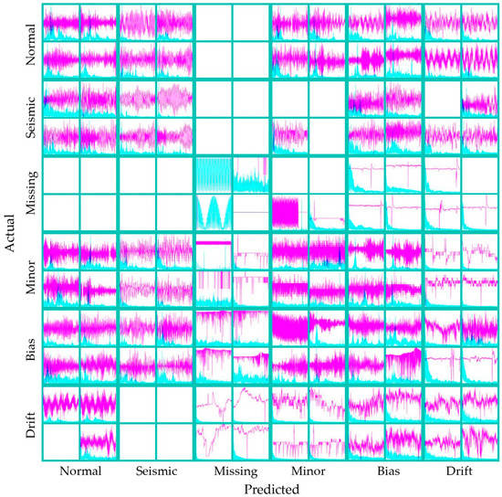
Figure 13.
Examples in detection results arranged by confusion matrix.
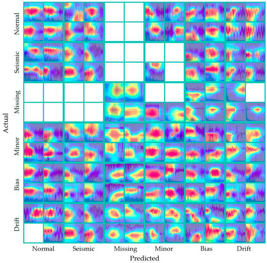
Figure 14.
Visualization of the confusion matrix of Figure 13.
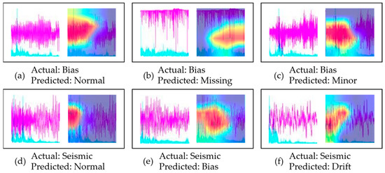
Figure 15.
Samples of classification errors.
The neural network also made some errors in detecting seismic samples, as shown in Figure 15d–f. Figure 15d captures the vibrations at the very beginning of the earthquake, which lies on the latter half of the sample. However, the neural network classified the sample as Normal based on the corresponding feature, which is located in the first half of the time series. In Figure 15e, the neural network mistakenly classified the Seismic sample as pattern Bias, neglecting the low-frequency features of seismic vibration. As for Figure 15f, the neural network mistook the long-period characteristics of earthquake response for drift features, leading to the misclassification as pattern Drift. Summarizing the aforementioned cases, an important reason for misclassification is that samples can contain multiple types of features simultaneously, making it difficult for the neural network to classify those samples. Therefore, a fine-grained segmentation for continuous time history, or a multi-label classification method should be considered.
5. Conclusions
This paper presents an interpretable vision-based deep learning method for identifying seismic events under the interference of multi-type anomalies. The raw time series was transformed into time- and frequency-response images, respectively, turning the seismic event and anomaly detection problem into an image classification task. Transfer learning was conducted based on the ResNet34, and the interpretation algorithm Grad-CAM was embedded for outputting understandable heat map to highlight the important region for classification. The novelty of the research is that both seismic data and faulty data are considered, which aims at the challenging issue in practical engineering applications. Additionally, not only classified labels, but also explainable visual information are provided, enhancing human trust in the decision-making of the neural network.
Four seismic monitoring datasets of a long-span cable-stayed bridge were used for method verification. The dataset contained not only normal and seismic data but also four anomaly patterns: Missing, Minor, Bias, and Drift. The results show that the seismic responses were successfully identified with a precision of over 80 percent and a recall of over 60 percent. The recognized earthquake starting time corresponded well with the groundtruth. Moreover, pattern Missing, Minor, and Drift were accurately identified, while the recall of pattern Bias was relatively low due to a large number of misclassified normal samples. Meanwhile, the regions of interest for each sample for classification were obtained, revealing that the neural network focused on low-level and discrete features at shallow layers, and high-level and holistic features at deep layers. Additionally, representative features for each pattern were discovered. By analyzing the heat maps, the reason for the misclassification of some samples was identified, namely the coexistence of multiple patterns features in the same sample. Therefore, we will investigate fine-grained image segmentation or a multi-label classification method to solve the problem.
Author Contributions
Conceptualization, Z.T.; methodology, Z.T.; software, J.G.; resources, C.Z. and W.X.; data curation, J.G.; writing—original draft preparation, J.G.; writing—review and editing, Z.T. and W.X.; supervision, Y.W.; project administration, W.X.; funding acquisition, Z.T. and C.Z. All authors have read and agreed to the published version of the manuscript.
Funding
This research was supported by the Yunnan Fundamental Research Projects (Grant No. 202301AT070394, 202101AU070032), and the Fund for Less Developed Regions of the National Natural Science Foundation of China (Grant No. 12162017).
Institutional Review Board Statement
Not applicable.
Informed Consent Statement
Not applicable.
Data Availability Statement
The data used to support the findings of this study are available from the corresponding author upon request.
Conflicts of Interest
The authors declare no conflict of interest.
References
- Sony, S.; Laventure, S.; Sadhu, A. A Literature Review of Next-generation Smart Sensing Technology in Structural Health Monitoring. Struct. Control Health Monit. 2019, 26, e2321. [Google Scholar] [CrossRef]
- Abdulkarem, M.; Samsudin, K.; Rokhani, F.Z.; Rasid, M.F.A. Wireless Sensor Network for Structural Health Monitoring: A Contemporary Review of Technologies, Challenges, and Future Direction. Struct. Health Monit. 2020, 19, 693–735. [Google Scholar] [CrossRef]
- Mei, H.; Haider, M.; Joseph, R.; Migot, A.; Giurgiutiu, V. Recent Advances in Piezoelectric Wafer Active Sensors for Structural Health Monitoring Applications. Sensors 2019, 19, 383. [Google Scholar] [CrossRef] [PubMed]
- Bao, Y.; Chen, Z.; Wei, S.; Xu, Y.; Tang, Z.; Li, H. The State of the Art of Data Science and Engineering in Structural Health Monitoring. Engineering 2019, 5, 234–242. [Google Scholar] [CrossRef]
- Balaban, E.; Saxena, A.; Bansal, P.; Goebel, K.F.; Curran, S. Modeling, Detection, and Disambiguation of Sensor Faults for Aerospace Applications. IEEE Sens. J. 2009, 9, 1907–1917. [Google Scholar] [CrossRef]
- Bao, Y.; Tang, Z.; Li, H.; Zhang, Y. Computer Vision and Deep Learning–Based Data Anomaly Detection Method for Structural Health Monitoring. Struct. Health Monit. 2019, 18, 401–421. [Google Scholar] [CrossRef]
- Tang, Z.; Chen, Z.; Bao, Y.; Li, H. Convolutional Neural Network-Based Data Anomaly Detection Method Using Multiple Information for Structural Health Monitoring. Struct. Control Health Monit. 2019, 26, e2296.1–e2296.22. [Google Scholar] [CrossRef]
- Saeed, U.; Jan, S.U.; Lee, Y.-D.; Koo, I. Fault Diagnosis Based on Extremely Randomized Trees in Wireless Sensor Networks. Reliab. Eng. Syst. Saf. 2021, 205, 107284. [Google Scholar] [CrossRef]
- Smarsly, K.; Law, K.H. Decentralized Fault Detection and Isolation in Wireless Structural Health Monitoring Systems Using Analytical Redundancy. Adv. Eng. Softw. 2014, 73, 1–10. [Google Scholar] [CrossRef]
- Jan, S.U.; Lee, Y.D.; Koo, I.S. A Distributed Sensor-Fault Detection and Diagnosis Framework Using Machine Learning. Inf. Sci. 2021, 547, 777–796. [Google Scholar] [CrossRef]
- Li, S.; Wei, S.; Bao, Y.; Li, H. Condition Assessment of Cables by Pattern Recognition of Vehicle-Induced Cable Tension Ratio. Eng. Struct. 2018, 155, 1–15. [Google Scholar] [CrossRef]
- Mao, J.; Wang, H.; Spencer, B.F. Toward Data Anomaly Detection for Automated Structural Health Monitoring: Exploiting Generative Adversarial Nets and Autoencoders. Struct. Health Monit. 2021, 20, 1609–1626. [Google Scholar] [CrossRef]
- Sun, Z.; Zou, Z.; Zhang, Y. Utilization of Structural Health Monitoring in Long-Span Bridges: Case Studies. Struct. Control Health Monit. 2017, 24, e1979. [Google Scholar] [CrossRef]
- Zhang, L.; Chen, P.; Li, M.; Chen, L.; Mou, J. A Data-Driven Approach for Ship-Bridge Collision Candidate Detection in Bridge Waterway. Ocean Eng. 2022, 266, 113137. [Google Scholar] [CrossRef]
- Lim, J.-Y.; Kim, S.; Kim, H.-K.; Kim, Y.-K. Long Short-Term Memory (LSTM)-Based Wind Speed Prediction during a Typhoon for Bridge Traffic Control. J. Wind Eng. Ind. Aerodyn. 2022, 220, 104788. [Google Scholar] [CrossRef]
- Gentili, S.; Michelini, A. Automatic Picking of P and S Phases Using a Neural Tree. J. Seismol. 2006, 10, 39–63. [Google Scholar] [CrossRef]
- Perol, T.; Gharbi, M.; Denolle, M. Convolutional Neural Network for Earthquake Detection and Location. Sci. Adv. 2018, 4, e1700578. [Google Scholar] [CrossRef]
- Ross, Z.E.; Meier, M.-A.; Hauksson, E.; Heaton, T.H. Generalized Seismic Phase Detection with Deep Learning. Bull. Seismol. Soc. Am. 2018, 108, 2894–2901. [Google Scholar] [CrossRef]
- Zhang, Y.; Wang, X.; Ding, Z.; Du, Y.; Xia, Y. Anomaly Detection of Sensor Faults and Extreme Events Based on Support Vector Data Description. Struct. Control Health Monit. 2022, 29, e3047. [Google Scholar] [CrossRef]
- Barkhordari, M.S.; Armaghani, D.J.; Asteris, P.G. Structural Damage Identification Using Ensemble Deep Convolutional Neural Network Models. Comput. Model. Eng. Sci. 2023, 134, 835–855. [Google Scholar] [CrossRef]
- Barkhordari, M.S.; Barkhordari, M.M.; Armaghani, D.J.; Rashid, A.S.A.; Ulrikh, D.V. Hybrid Wavelet Scattering Network-Based Model for Failure Identification of Reinforced Concrete Members. Sustainability 2022, 14, 12041. [Google Scholar] [CrossRef]
- Arrieta, A.B.; Díaz-Rodríguez, N.; Del Ser, J.; Bennetot, A.; Tabik, S.; Barbado, A.; García, S.; Gil-López, S.; Molina, D.; Benjamins, R.; et al. Explainable Artificial Intelligence (XAI): Concepts, Taxonomies, Opportunities and Challenges toward Responsible AI. Inf. Fusion 2019, 58, 82–115. [Google Scholar] [CrossRef]
- Xu, K.; Liu, S.; Zhang, G.; Sun, M.; Zhao, P.; Fan, Q.; Gan, C.; Lin, X. Interpreting Adversarial Examples by Activation Promotion and Suppression. arXiv 2019, arXiv:1904.02057. [Google Scholar]
- Selvaraju, R.R.; Cogswell, M.; Das, A.; Vedantam, R.; Parikh, D.; Batra, D. Grad-CAM: Visual Explanations from Deep Networks via Gradient-Based Localization. Int. J. Comput. Vis. 2020, 128, 336–359. [Google Scholar] [CrossRef]
- Dosovitskiy, A.; Brox, T. Inverting Visual Representations with Convolutional Networks. In Proceedings of the 2016 IEEE Conference on Computer Vision and Pattern Recognition (CVPR), Las Vegas, NV, USA, 27–30 June 2016; IEEE: Las Vegas, NV, USA, 2016; pp. 4829–4837. [Google Scholar]
- Panwar, H.; Gupta, P.K.; Siddiqui, M.K.; Morales-Menendez, R.; Bhardwaj, P.; Singh, V. A Deep Learning and Grad-CAM Based Color Visualization Approach for Fast Detection of COVID-19 Cases Using Chest X-Ray and CT-Scan Images. Chaos Solitons Fractals 2020, 140, 110190. [Google Scholar] [CrossRef]
- Xiao, G. FCSNet: A Quantitative Explanation Method for Surface Scratch Defects during Belt Grinding Based on Deep Learning. Comput. Ind. 2023, 144, 103793. [Google Scholar] [CrossRef]
- Zhang, Y.; Miyamori, Y.; Mikami, S.; Saito, T. Vibration-based Structural State Identification by a 1-dimensional Convolutional Neural Network. Comput.-Aided Civ. Infrastruct. Eng. 2019, 34, 822–839. [Google Scholar] [CrossRef]
- Yang, R.; Singh, S.K.; Tavakkoli, M.; Amiri, N.; Yang, Y.; Karami, M.A.; Rai, R. CNN-LSTM Deep Learning Architecture for Computer Vision-Based Modal Frequency Detection. Mech. Syst. Signal Process. 2020, 144, 106885. [Google Scholar] [CrossRef]
- Canizo, M.; Triguero, I.; Conde, A.; Onieva, E. Multi-Head CNN–RNN for Multi-Time Series Anomaly Detection: An Industrial Case Study. Neurocomputing 2019, 363, 246–260. [Google Scholar] [CrossRef]
- He, K.; Zhang, X.; Ren, S.; Sun, J. Delving Deep into Rectifiers: Surpassing Human-Level Performance on ImageNet Classification. In Proceedings of the 2015 IEEE International Conference on Computer Vision (ICCV), Santiago, Chile, 7–13 December 2015; IEEE: Santiago, Chile, 2015; pp. 1026–1034. [Google Scholar]
- Liu, L.; Liu, X.; Gao, J.; Chen, W.; Han, J. Understanding the Difficulty of Training Transformers. arXiv 2020, arXiv:2004.08249. [Google Scholar]
- Basodi, S.; Ji, C.; Zhang, H.; Pan, Y. Gradient Amplification: An Efficient Way to Train Deep Neural Networks. Big Data Min. Anal. 2020, 3, 196–207. [Google Scholar] [CrossRef]
- He, K.; Zhang, X.; Ren, S.; Sun, J. Deep Residual Learning for Image Recognition. In Proceedings of the 2016 IEEE Conference on Computer Vision and Pattern Recognition (CVPR), Las Vegas, NV, USA, 27–30 June 2016; IEEE: Las Vegas, NV, USA, 2016; pp. 770–778. [Google Scholar]
- Zhuang, F.; Qi, Z.; Duan, K.; Xi, D.; Zhu, Y.; Zhu, H.; Xiong, H.; He, Q. A Comprehensive Survey on Transfer Learning. arXiv 2020, arXiv:1911.02685. [Google Scholar] [CrossRef]
- Pan, S.J.; Yang, Q. A Survey on Transfer Learning. IEEE Trans. Knowl. Data Eng. 2010, 22, 1345–1359. [Google Scholar] [CrossRef]
- Xu, Y.; Bao, Y.; Zhang, Y.; Li, H. Attribute-Based Structural Damage Identification by Few-Shot Meta Learning with Inter-Class Knowledge Transfer. Struct. Health Monit. 2021, 20, 1494–1517. [Google Scholar] [CrossRef]
- Lin, Y.-P.; Jung, T.-P. Improving EEG-Based Emotion Classification Using Conditional Transfer Learning. Front. Hum. Neurosci. 2017, 11, 334. [Google Scholar] [CrossRef]
- Du, Y.; Li, L.; Hou, R.; Wang, X.; Tian, W.; Xia, Y. Convolutional Neural Network-Based Data Anomaly Detection Considering Class Imbalance with Limited Data. Smart Struct. Syst. 2022, 29, 63–75. [Google Scholar]
- Tajbakhsh, N.; Shin, J.Y.; Gurudu, S.R.; Hurst, R.T.; Kendall, C.B.; Gotway, M.B.; Liang, J. Convolutional Neural Networks for Medical Image Analysis: Full Training or Fine Tuning? IEEE Trans. Med. Imaging 2016, 35, 1299–1312. [Google Scholar] [CrossRef]
- Zhou, B.; Khosla, A.; Lapedriza, A.; Oliva, A.; Torralba, A. Learning Deep Features for Discriminative Localization. In Proceedings of the 2016 IEEE Conference on Computer Vision and Pattern Recognition (CVPR), Las Vegas, NV, USA, 27–30 June 2016; IEEE: Las Vegas, NV, USA, 2016; pp. 2921–2929. [Google Scholar]
- Siringoringo, D.M.; Fujino, Y.; Namikawa, K. Seismic Response Analyses of the Yokohama Bay Cable-Stayed Bridge in the 2011 Great East Japan Earthquake. J. Bridge Eng. 2014, 19, A4014006. [Google Scholar] [CrossRef]
Disclaimer/Publisher’s Note: The statements, opinions and data contained in all publications are solely those of the individual author(s) and contributor(s) and not of MDPI and/or the editor(s). MDPI and/or the editor(s) disclaim responsibility for any injury to people or property resulting from any ideas, methods, instructions or products referred to in the content. |
© 2023 by the authors. Licensee MDPI, Basel, Switzerland. This article is an open access article distributed under the terms and conditions of the Creative Commons Attribution (CC BY) license (https://creativecommons.org/licenses/by/4.0/).

