Wearable-Based Intelligent Emotion Monitoring in Older Adults during Daily Life Activities

Abstract

We present a system designed to monitor the well-being of older adults during their daily activities. To automatically detect and classify their emotional state, we collect physiological data through a wearable medical sensor. Ground truth data are obtained using a simple smartphone app that provides ecological momentary assessment (EMA), a method for repeatedly sampling people’s current experiences in real time in their natural environments. We are making the resulting dataset publicly available as a benchmark for future comparisons and methods. We are evaluating two feature selection methods to improve classification performance and proposing a feature set that augments and contrasts domain expert knowledge based on time-analysis features. The results demonstrate an improvement in classification accuracy when using the proposed feature selection methods. Furthermore, the feature set we present is better suited for predicting emotional states in a leave-one-day-out experimental setup, as it identifies more patterns.

1. Introduction

We are experiencing unprecedented social and demographic changes. According to the United Nations, the world’s population is expected to increase to 9.7 billion by 2050, with 2 billion being people aged 60 or above [1,2]. In Europe, there will be around 151 million people aged over 65 years by 2060.

More and more, older citizens wish to stay in their homes for as long as possible in order to enjoy an active and healthy aging life [3]. However, older adults living alone are more likely to experience poor mental health, including depression, anxiety or low self-esteem [4]. In fact, depression is the main mental illness ahead of dementia in older adults, and the major cause of suicide in this population [5]. More recently, the pandemic has had a great impact on their mental health conditions [5]; in particular, perceived social isolation results in significant negative consequences related to mental well-being [6].

Although there is an increasing acknowledgment of the important role of mental health in the daily life of people, it still has relatively low priority in older adults; it has been poorly covered by existing health-monitoring systems; and it is often considered a forgotten matter [7,8]. In addition, there will be future shortages of available health workers and doctors to cover all demands for home assistance, mainly due to population aging and low birth rations [5,9]. Therefore, there is an urgent need for new and innovative forms to support the mental well-being of older adults.

Healthcare systems that incorporate wearable sensing technologies are emerging as an alternative method to meet future demands for distance and personalized medicine. Moreover, the application of artificial intelligence (AI) to endow machines with the perception of human affects, i.e., affective computing, is also receiving increased attention as a way of monitoring and predicting the well-being of people during their daily life [10]. Later in the text, we refer indifferently to the emotional or affective state as a component of well-being, despite the differences between the terms as presented in [11].

In this paper, we present an AI-based system (see Figure 1) to monitor the emotions of older adults during their daily life, with the goal of preserving their mental and emotional well-being. Our system is composed of the wearable watch-like Empatica E4 certified medical sensor [12] that collects several physiological and activity signals. Those signals are processed and converted into feature vectors that are classified into one of the affective concepts [13], which provide evidence of the mental well-being of the participants.

To collect ground truth data from older adults to train the supervised classifier, we provided an app for the smartphone that includes an ecological momentary assessment (EMA) tool, allowing for quick and unobtrusive user input [14]. This tool simplifies the emotional state assessment of the participant by asking two simple questions related to levels of valence and arousal, each measured on a 5-point Likert scale.

Our contributions with this work are as follows: (1) two feature selection methods whose results prove to work efficiently in discriminating different affective states; (2) a feature set that disregards domain expert knowledge during the feature engineering step; and (3) a thorough methodology evaluation using a collection of different classification methods in two experimental setups. Based on the experiments, we concluded future steps to improve healthcare systems based on bio-wearable sensors.

2. Related Work

There are several modalities to predict or monitor mental well-being and the affective state that include visual [15], textual [16] or speech [17]. Nevertheless, these modalities’ trustworthiness can be compromised by a phenomenon known as social masking [18], which refers to the fact that participants can unconsciously or deliberately hide real emotions, i.e., faking a face gesture, or modulating voice’s tonality. For this reason, physiological data are used in a wide range of studies to assess not only emotions but also stress or anxiety states [18].

Picard et al. introduced in [10] the importance of endowing computers with the ability to understand and recognize human affective states by analyzing four different physiological signals. Since then, many efforts have been made to improve human–computer interactions [10]. Moreover, the authors in [19] monitored depressive moods by using EMA questionnaires to train different machine learning models from wearable lifestyle data, such as sleep, physical activity and physiological signals. In [20], the authors used the circumplex model of affect, presented by Russell et al. [13], to label emotions. However, the proposed model is trained to predict only three different emotions: sadness, happiness, and neutrality. In this work, we discretize the circumplex model of affect [13] in eight different emotions: pleasure, excitement, arousal, distress, misery, depression, sleepiness, and contentment.

There is an increasing interest in the use of wearable devices to collect physiological data. Many commercial wearable sensors have been used to predict and monitor emotions [21,22]. However, for our work, we used the Empatica E4 [12] medical-certified wearable device. In [23], the authors proposed laboratory-based experiments using the Empatica E4 sensor to collect data and extract meaningful emotion-based features to feed a neural network. In addition, the work in [24] proposed two different architectures to process four physiological signals gathered from the Empatica E4 device using a public data benchmark [25]. The authors in [26] used Empatica E4 to collect physiological signals in an experiment to study blue light as a factor to reduce stress. In [27], the authors collected heart rate variability signals through the E4 to train different machine learning classifiers, with the goal of predicting emotions elicited in a virtual reality environment. The authors in [28] conducted a similar experiment to the one presented in this work by using data collected from the Empatica E4 sensor to detect affective changes in participants. They used controlled scenarios to induce emotional states during the experiment, having full control of the environment. In contrast, we did not control the participants’ activities during data collection.

All works mentioned previously followed a laboratory-based approach, that is, a controlled environment to collect data. Recent research [29] encouraged the importance of collecting data in non-controlled scenarios, also called in-the-wild environments. Few works have followed this approach [29]. For example, stress was addressed in [30], where the authors only analyzed a set of fixed activities of the daily life to be studied. On the contrary, in our work, we had no control over participants’ activities during the collection of data, being that the data analysis task was more challenging and representative of real life. Additionally, in [31], in-the-wild physiological data were collected, which were combined with context information to define the perceived stress levels of individuals. In [32], the authors monitored changes in depression severity by combining physiological features extracted from the Empatica E4 device and behavioral features obtained from smartphones.

In our approach, the feature vectors are selected from a pool of standard time-based features used in the time analysis using the tsfresh library [33]. Similar approaches have been used in other works, analyzing different physiological signals. For example, in [34], the authors used this library to extract features from raw electroencephalography (EEG) signals to detect epileptic seizures. The work in [35] used the same library to compute features from EEG biomarkers, proposing a fully automated machine learning pipeline to assess cognition deterioration. Moreover, the authors in [36] used this library to extract, among others, features from a smartphone’s accelerometer to predict mood. Finally, in [37], the authors extracted features from heart rate using the tsfresh tool to detect heart-related anomalies.

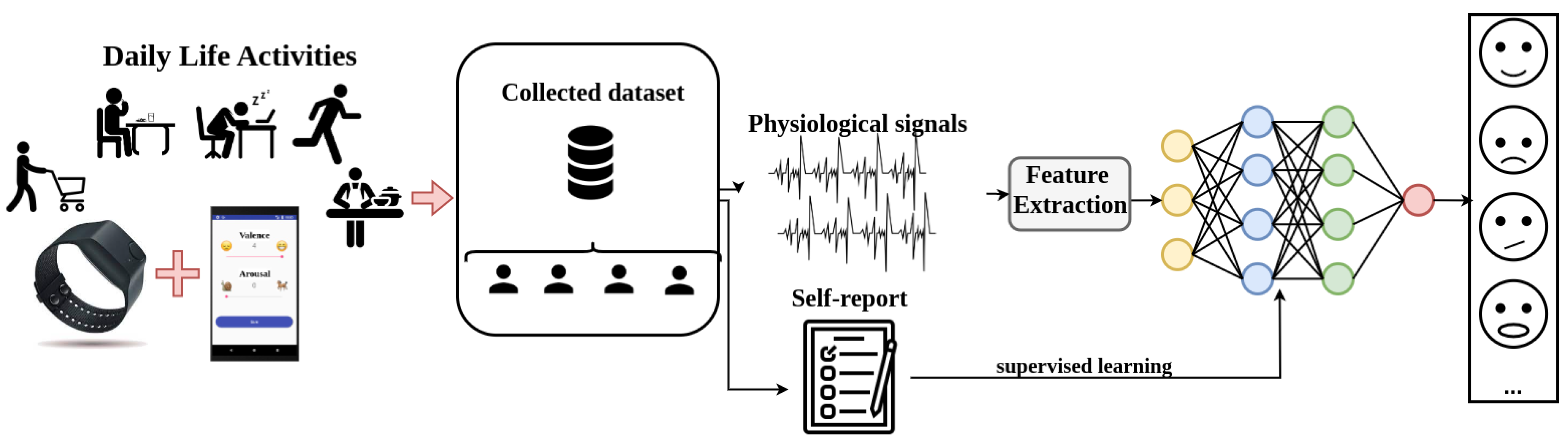
3. Emotional State Monitoring Methodology

3.1. Sensor Description

Physiological data can provide valuable information about subtle changes in the activation of the autonomic nervous system caused by an emotional stimulus [18]. For this reason, we used a medical wearable sensor as described in this section.

We collected physiological data from participants using the wearable device Empatica E4 [12], which is a non-obtrusive medical-certified device in the form of a watch that is worn on the wrist (Figure 2). Empatica E4 provides the following sensors and corresponding signals:

• Photoplethysmogram (PPG) sensor. This sensor measures the blood volume pulse (BVP), i.e., the variation of volume of arterial blood under the skin resulting from the heart cycle, which is sampled at $64\mathrm{Hz}$. This signal is used to derive the heart rate variability (HRV) which is computed by a built-in internal function within the wearable device. The sampling rate corresponding to the HRV signal is 1 $\mathrm{Hz}$.
• Electrodermal activity (EDA) sensor. This sensor measures the variations in electrical conductance of the skin as a response to sweat secretion, which is a potential response of the autonomic nervous system to a stimulus. Data are sampled at a fixed frequency of 4 $\mathrm{Hz}$. This signal is filtered using a 3rd order low-pass Butterworth filter with a cut-off frequency of $1.5$ $\mathrm{Hz}$. In addition, the signal is decomposed into two signals: the skin conductance level (SCL), and the skin conductance response (SCR) [38].
• Infrared thermophile sensor. This sensor measures the peripheral skin temperature variations. Data are sampled at a frequency of 4 $\mathrm{Hz}$.
• 3-axis accelerometer. This sensor records wrist motion data in the carrier’s x, y, and z axes, which are sampled at 32 $\mathrm{Hz}$. Additionally, we calculate the Euclidean norm of the three collected axes. Finally, we apply a Butterworth filter with cut-off frequencies of $0.2$ $\mathrm{Hz}$ and 410 $\mathrm{Hz}$ [39].

Raw signals were anonymously uploaded to a controlled cloud environment by the participants. After the experiment period, they were downloaded for processing, feature extraction, and classification (all data are collected, stored and processed in accordance with the GDPR regulations).

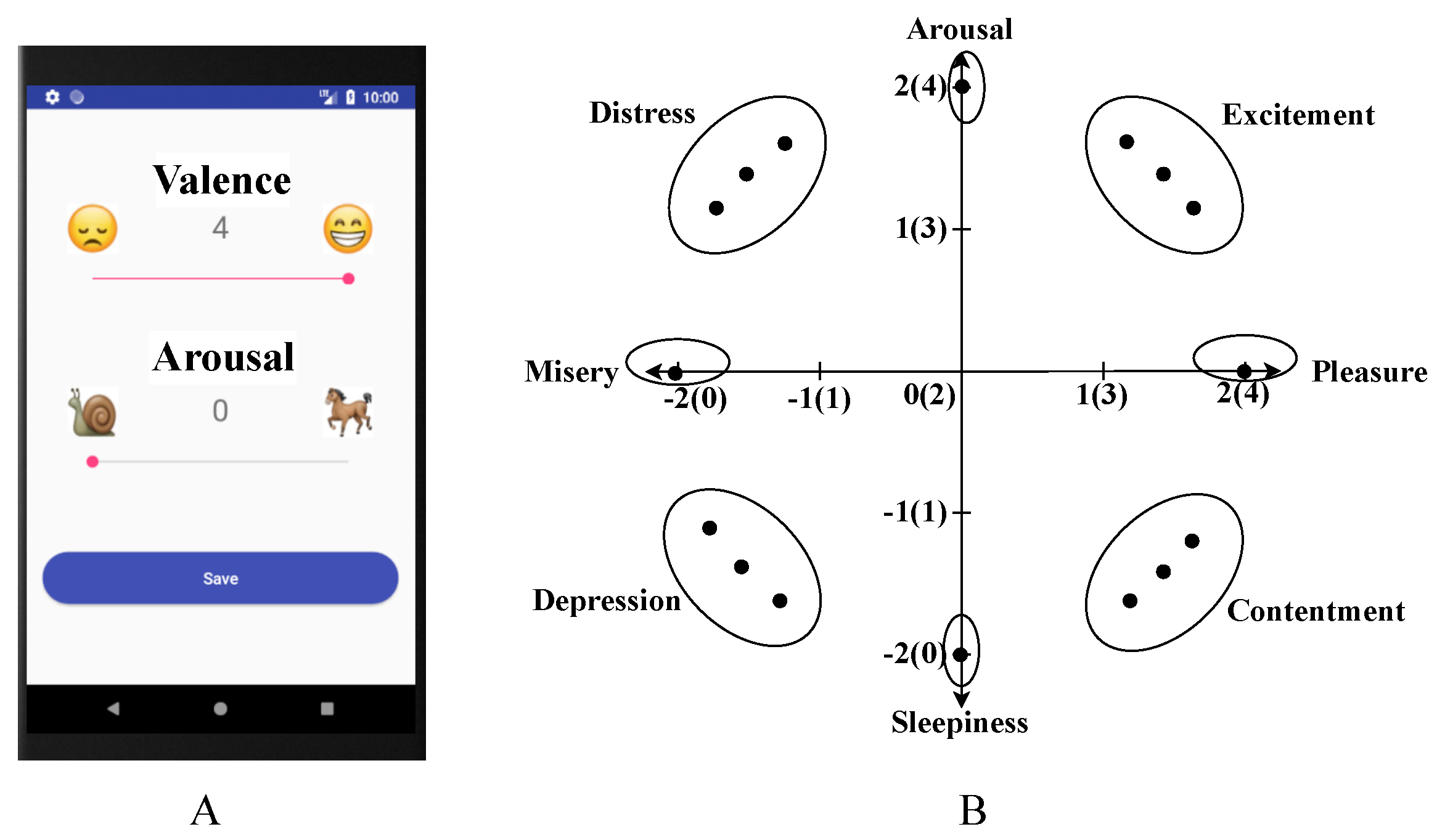
3.2. Data Annotation

In order to train our supervised classifier, we annotated our data with the emotional state of the person at several moments of the day during their daily activities. In clinical psychology, mental assessment relies on retrospective reports, which normally are subject to recall bias. However, as noted by Shiffman et al. [40], this approach limits the ability to precisely characterize, understand, and change the behavior in real-world conditions. In order to minimize the impact of those limits, we used ecological momentary assessment (EMA), in which very short questions are asked to the participant at different times during their daily life activities, as used in [41] to monitor teachers’ emotional states and behaviors over time. This approach aims to study peoples’ affective states in their daily lives by repeatedly gathering data in an individual’s normal environment.

Following previous works [20,42,43], we used the circumplex model of affect introduced by J. A. Russell [13], which describes affective states as a bi-dimensional model guided by two dimensions, valence and arousal, as shown in Figure 3. This model is validated and represents the participant’s emotional self-subjective evaluation. Following the guidelines from [44], we designed an app for the smartphone that used the measurements valence and arousal in a 5-point Likert scale, ranging from 0 to 4. Dimensional affective models, i.e., those which define affective states from different dimensions (valence and arousal), are more reliable than models based on discrete categories, i.e., asking directly affective categories, such as anger and fear, as stated in [45]. For this reason, we calculated the final affective state, which was obtained by interpolating the valence or pleasure and arousal levels as explained in [13]. The app’s interface was kept simple to facilitate usage and to reduce attention theft, i.e., the shift of the user’s attention only to the device rather than the real environment. In order to avoid generating extra anxiety due to a high load of questions [44], users were asked only five times per day about their valence and arousal levels. In addition, participants were free to input their levels at any time.

3.3. Dataset Construction

Data were collected from participants during their daily life activities. The E4 sensor was provided to participants with the instruction to wear it as much as possible during the day. During the night, the device was charged, and data were transferred. Participants had the option to disconnect the wearable device at any time, such as when engaging in highly private activities, when the E4 sensor was inconvenient for the activity being performed, or when there was a risk of damaging the sensor (e.g., during showering).

We collected data from four older adults, focusing on personal models, which prioritized collection time over the quantity of participants. We believe that the number of days designated to collect data is sufficient to capture changes in the participants’ affective states during their daily activities.

Table 1. Summary of participants’ collected data.

	P1	P2	P3	P4
Age	67	55	60	63
Gender	Male	Female	Male	Female
Days	9	15	12	13
Total EMAs	42	57	64	46
Avg. EMAs	4.67	3.80	5.33	3.54

shows details for each participant and the corresponding collected data. The age of participants ranged between 55 and 67 years old. Gender was balanced in the dataset. Initially, we asked the participants to wear the sensor for two weeks; however, different participants wore it for a different number of days due to personal reasons. We can also see in Table 1 that participants answered an average per day of 3.54 to 5.33 times to the EMA questions. They were free to answer more times, and this had the possibility of resulting in an average bigger than 5, as occurred for participant P3.

For each participant, we collected the physiological data and the corresponding EMA inputs, which were aligned using timestamps. Ground truth is composed of the input levels of valence and arousal (levels 0 to 4). From these levels, we extrapolated the emotional state using Russel’s circumplex model [13]. We projected all possible combinations of valence–arousal pairs into the circle (see Figure 3B). As it can be observed in the figure, some valence–arousal projections are significantly close. We grouped them into the following emotional states: (1) pleasure, (2) excitement, (3) arousal, (4) distress, (5) misery, (6) depression, (7) sleepiness, and (8) contentment. These affective states were used in [13] to validate Russell’s affective theory. For this reason, as well as data scarcity, we decided to used them in our experiments.

Different participants reported different numbers of affective or emotional states, and this resulted in an imbalanced distribution of labels per participant among the possible classes. This imbalance is justified due to the nature of the collected data: different people feel different emotional states during their daily life activities. Moreover, we carried out experiments on healthy participants. Therefore, we expected the labels to be imbalanced between positive and negative states, with positive states being more dominant, as our participants demonstrated a healthy condition in the questionnaires administered prior to data collection (see Figure 4). This imbalance affects the generalization capabilities discussed in the following section.

The approach to collect data followed in this work differs from data collected in the lab, in that we did not have full control of the induced emotions or affective states. This dataset aims to collect emotional states in the wild. For this reason, we asked about the levels of arousal and valence since they represent a subjective assessment of the inner affective or emotional state, and it is an effective method when reporting affective states under these conditions [45].

The dataset presented in this work represents the actual challenge of emotional state monitoring, where such states appear in a natural and realistic environment. There is a lack of work under this type of setup as reported in [29]; therefore, we will make our dataset available on the internet for future comparisons and methods. Links to the dataset and the code to process it will be made public after the acceptance decision.

4. Feature Engineering for Affection Recognition

In this work, we opted for a feature-based approach to learn patterns in data that represent emotional or affective states. The amount of data available prohibits the training of deep models as convolutional neural networks or recursive neural networks [46] to extract meaningful feature spaces. This section introduces the feature engineering methodology to process the collected raw bio-signals.

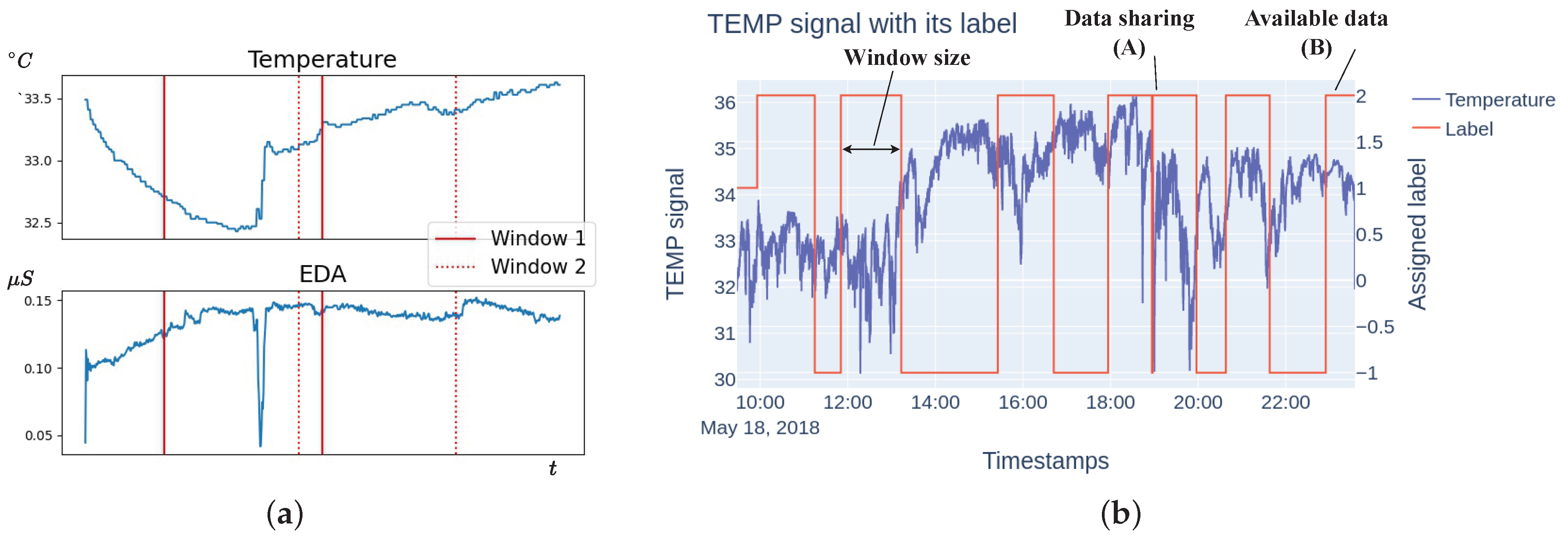
4.1. Feature Extraction and Labeling

In order to train and classify the temporal physiological signals, we first split them using a sliding window approach. The window size is selected to be 60 s since it is the most common size used for physiological signal analysis [47,48,49]. In addition, we set an overlapping of 10% between consecutive windows to reduce the boundary effect that appears when signals are filtered (see Figure 5a). We discard any window that is not fully filled for 60 s.

For each window, we extracted a set of features. Each modality or bio-signal was processed independently. Thus, we computed the features for each modality. Once features were extracted, we concatenated features from all modalities into a single vector. Previous work used specific medical-based features to solve this problem. For example, the authors in [14] extracted dedicated features for each modality, thus requiring expert domain knowledge. This feature set consisted of 203 features, and we used this as the baseline. For more details about this feature set, refer to [14]. In contrast, in this work, we extracted the same feature set per bio-signal. The extracted proposed set contains features used in temporal signal analysis [50]. For each window, we extracted 787 features for each sensor modality. This amount of features was predefined in [33]. We concatenated the extracted features from the 9 temporal signals (x, y, z, $norm$ axes, temperature, heart rate, EDA, SCL, and SCR) into a final feature vector of 7083 features. To extract the general time-based features, we used the tsfresh library [33].

To assign the ground truth label to each feature vector, we needed to align the physiological signals with the EMA input in the app. Each EMA response (valence and arousal levels) represents the emotional state of the participant at one point in time, and thus we obtained the ground truth label only for that specific timestamp. To obtain more labels, we followed [14] and expanded the label through a time window around the answer’s timestamp of 60 min. The latter window duration was supported by [51], where the authors concluded that emotions last between ten minutes and one hour, and the average duration of an emotion is 30 min.

As explained in Section 3.2, we asked participants five times during each day. However, the participants did not always answer on time. This created shifts in the response time. Moreover, participants were also free to provide extra answers anytime. This creates the potential situation of two consecutive EMA answers being closer in time than half the EMA window. In this case, the available data points are shared equally between the two EMA answers. Additionally, for the first and last EMA of the day, which were often answered within the first and last hour of the day, we selected the amount of data available. In Figure 5b we show examples of these situations.

4.2. Feature Selection

The number of features in the final feature vectors for each window is 7083, which is higher than the number of available labeled data available for each of the participants (see Section 4.1). This can cause a dimensionality problem when training our classifiers [52]. For that reason, we propose two features selectors approaches, described below.

4.2.1. Scalable Hypothesis Test Feature Selection

The feature selection based on scalable hypothesis tests [50] consists of applying a singular statistical test to each feature $\{x_1,\dots ,x_{\varphi },\dots ,x_{n_{\varphi }}\}$ to check the following hypothesis:

$$\begin{array}{cc}\hfill & H_0^{\varphi }=x_{\varphi }\mathrm{i}\mathrm{s}\mathrm{i}\mathrm{r}\mathrm{r}\mathrm{e}\mathrm{l}\mathrm{e}\mathrm{v}\mathrm{a}\mathrm{n}\mathrm{t}\mathrm{f}\mathrm{o}\mathrm{r}\mathrm{p}\mathrm{r}\mathrm{e}\mathrm{d}\mathrm{i}\mathrm{c}\mathrm{t}\mathrm{i}\mathrm{n}\mathrm{g}\mathrm{Y},\hfill \\ \hfill & H_1^{\varphi }=x_{\varphi }\mathrm{i}\mathrm{s}\mathrm{r}\mathrm{e}\mathrm{l}\mathrm{e}\mathrm{v}\mathrm{a}\mathrm{n}\mathrm{t}\mathrm{f}\mathrm{o}\mathrm{r}\mathrm{p}\mathrm{r}\mathrm{e}\mathrm{d}\mathrm{i}\mathrm{c}\mathrm{t}\mathrm{i}\mathrm{n}\mathrm{g}\mathrm{Y},\hfill \end{array}$$

(1)

where Y is the EMA label assigned to feature vector $x_{\varphi }$, $\varphi$ being the index of the feature. Basically, this approach consists of treating each extracted feature independently and performing a statistical test on it, which will differ among features depending on whether the targets and features are binary or not. As a result, we obtained a vector with p-values $\{p_1,\dots ,p_{n_{\varphi }}\}$, which was used to select the final features using different testing approaches. In this work, we use the Kolmogorov–Smirnov test [53] for binary extracted features, and the Kendall rank test [54] for non-binary extracted features, as it is detailed in [50]. We used the implementation provided in the tsfresh library [33].

We proposed a feature reduction method based on common features. The selected feature set varies when the selection is made among different features sets. Our intuition is that there should be common features among those different sets when the training data come from the same source, e.g., the same participant. In order to check this idea, we devised a feature selection process in which we divide the training data into different subsets. For each subset, we apply the previous feature selector, obtaining a vector of intermediate selected features corresponding to each subset. Then we locate the common features among those intermediate feature vectors to select the final set of features. The specific steps are as follows:

• The training set $S_{train}$ with feature size 7083, is bagged into Z disjoints subsets $S_{train}=\{S_1,...,S_Z\}$.
• We select features from each subset $S_z$ and obtained Z vectors of selected features $\{{\mathbf{f}}_1,...,{\mathbf{f}}_Z\}$ using the scalable hypothesis method.
• We search for the common features among all ${\mathbf{f}}_z$ vectors obtaining the final feature vector ${\mathbf{f}}_{common}$.

This final feature vector ${\mathbf{f}}_{common}$ is fed to the supervised classifier. We train personal models, and thus this feature vector is different for each participant.

4.2.2. Mutual Information Feature Selection

The feature selection introduced previously evaluates each feature independently. Thus, the selecting is unable to deal with redundant or jointly relevant features. To overcome this problem, we compare to a feature selector based on the idea introduced in [55]. This algorithm uses mutual information (MI) [56] to select non-redundant features for the classification task.

In each round, the MI algorithm selects the feature that best explains the misclassified samples, and adds it to the feature set. This process continues until no further improvement in classification accuracy is achieved for 50 consecutive rounds. Therefore, the features are ranked according to the MI between the samples and labels, and the highest-ranked feature is added to the set of selected features. Then, a classifier is trained based on all samples and the selected features. All correctly classified samples are removed from the MI computation for the following round, and the algorithm repeats. Intuitively speaking, in each round, the algorithm finds the feature that explains the currently wrongly classified samples best, somewhat like the AdaBoost algorithm. In Algorithm 1, we show the pseudo-code of this feature selector. We highlight again that we train personal models, and thus the selected feature set is different among participants.

Algorithm 1 Feature selection based on mutual information

1: Input: X, y [training samples and labels] 2: Output: S, m [selected feature set and trained model] 3: Initialize: $S\leftarrow \varnothing$ 4:             $X^{*},y^{*}\leftarrow X,y$ 5:             $criterion\leftarrow False$ 6: repeat 7:      $F_{max}\leftarrow \underset{F_i}{argmax}MI(X^{*},y^{*})$       ▹ determine feature with highest MI 8:      $S\leftarrow F_{max}$         ▹ add feature in selected feature set S 9:      $x_{cc},y_{cc}\leftarrow cls(X^S,y^S)$  ▹ get correctly classified (cc) samples using S feature set 10:     $X^{*}\leftarrow X^{}\setminus x_{cc}$; $y^{*}\leftarrow y^{}\setminus y_{cc}$         ▹ remove correctly classified samples from set 11:     CheckStopCriteria()          ▹at the end of each round, check stop criteria 12: until  $criterion\leftarrow True$

5. Emotional Predictive Models

5.1. Classification

Due to the complexity of the data, we carried out a thorough evaluation by training a battery of different classic machine learning algorithms. We highlight the following models: support vector machine (SVM) with radial basis function as kernel, random forest (RF), and multilayer perceptron (MLP). We applied grid search to find optimal parameters of each model (see

Table 2. Grid search parameter space for each model.

Model	Parameter Setting
SVM	C:[1,3,5,7,9]; $\gamma$:[1e-2, 1, in steps of 0.1]
RF	n_estimators: [200, 500]; max_features: [’sqrt’]; max_depth: [2, 4, 8]; criterion: [’gini’,’entropy’]
MLP	hidden_layer_sizes: [(250, 150), (150,)]; activation: [’tanh’, ’relu’]; solver: [’adam’]; learning_rate: [’adaptive’]

for a detailed description of the parameter search space). Prior to testing the final model, we validated and fine-tuned the model’s parameters using a stratified 10-fold cross-validation approach. This dataset is clearly imbalanced. However, this is expected, i.e., people tend to stay in neutral or positive affective states more often than in negative ones. To address this, we used the F1-score as a metric to find an optimal combination of parameters for the model.

Since our goal is to obtain a personal model for each participant, we trained a classifier using the data collected from each participant individually. Each individual emotional state model was learned using two different experimental setups. In the first one, we divided the complete set of data into 75% for training and 25% for testing. For the second setup, we applied a leave-one(day)-out strategy, in which we used one full day of data for testing, and trained using data from the rest of the days. We use the first approach as a simple division strategy to evaluate the performance of our method. The second approach is the real challenge to solve since it mimics real life. We emphasize that the second approach did not learn any information from the first one.

Our experiments aim to compare the performance of the selecting methods introduced in the previous section on the proposed time-analysis-based feature set with respect to the medical-based handcrafted features presented in [14]. For better understanding, we remark here the nomenclature followed in the results section. We denote baseline as the medical-based handcrafted feature set [14]. We refer to the time-analysis-based feature set as ours. The feature selectors are denoted in the following way: $f_{common}^n$ for the selector based on common features explained in Section 4.2.1, where n indicates the number of disjoints subsets; and $f_{MI}$ for the selector based on mutual information explained in Section 4.2.2. To indicate that a feature selector was used with any of the feature sets, we use the following form: $f_{common}^3\left(ours\right)$. The latter denotes the use of common features selector using 3 disjoints sets on the feature set we propose.

5.2. Results

In this section, we show the results of applying our method to the problem of emotion detection in the wild using our provided dataset. In the experiments, we used as a baseline the results obtained from the set of features proposed in [14]. We assessed our proposed feature set based on generic time series features by applying the feature selectors explained in Section 3. For the selection based on common features, we used 3 disjoints sets. We remark again that all trained models are bespoke, that is, we used each participant’s data individually to train the classifier.

In the first experiment, we followed a simple strategy to separate train and test sets. We randomly split the data into 75% for training and 25% for testing. This split was performed in a stratified way to keep similar distribution of labels between training and testing sets. For validation, we used 10-fold cross validation as explained in Section 5.1. We repeated this process 10 times for each participant and calculated the average F1-score (expressed in percentage), which combines the precision and recall of a classifier into a simple metric by taking their harmonic mean [57], and is a suitable metric for imbalanced datasets. This experiment was used to do a first evaluation of the proposed feature set and selection methods. In

Table 3. Results for the simple strategy experiment (F1-score expressed in percentage).

SVM					RF				MLP
	$\mathit{baseline}$	${\mathit{f}}_{\mathit{common}}^{\mathit{1}}\left(\mathit{ours}\right)$	${\mathit{f}}_{\mathit{common}}^{\mathit{3}}\left(\mathit{ours}\right)$	${\mathit{f}}_{\mathit{mi}}\left(\mathit{ours}\right)$	$\mathit{baseline}$	${\mathit{f}}_{\mathit{common}}^{\mathit{1}}\left(\mathit{ours}\right)$	${\mathit{f}}_{\mathit{common}}^{\mathit{3}}\left(\mathit{ours}\right)$	${\mathit{f}}_{\mathit{mi}}\left(\mathit{ours}\right)$	$\mathit{baseline}$	${\mathit{f}}_{\mathit{common}}^{\mathit{1}}\left(\mathit{ours}\right)$	${\mathit{f}}_{\mathit{common}}^{\mathit{3}}\left(\mathit{ours}\right)$	${\mathit{f}}_{\mathit{mi}}\left(\mathit{ours}\right)$
P1	$65.00\pm 2.30$	$60.76\pm 17.00$	$72.15\pm 5.89$	$78.42\pm 6.10$	$76.86\pm 1.15$	$77.38\pm 5.08$	$78.18\pm 5.11$	$87.67\pm 1.61$	$69.32\pm 2.45$	$52.43\pm 22.86$	$54.93\pm 32.18$	$83.04\pm 2.08$
P2	$64.36\pm 2.24$	$54.27\pm 21.60$	$73.35\pm 5.62$	$77.25\pm 2.98$	$74.25\pm 2.90$	$78.65\pm 4.91$	$79.02\pm 4.73$	$79.90\pm 1.34$	$67.55\pm 3.34$	$56.51\pm 22.81$	$58.12\pm 22.61$	$75.50\pm 4.61$
P3	$68.27\pm 5.87$	$74.54\pm 6.31$	$75.95\pm 7.33$	$84.16\pm 1.57$	$74.48\pm 2.55$	$80.43\pm 5.99$	$81.61\pm 6.70$	$87.84\pm 2.81$	$66.90\pm 5.81$	$58.80\pm 22.31$	$59.29\pm 21.67$	$88.42\pm 0.56$
P4	$66.97\pm 5.89$	$76.42\pm 7.17$	$76.57\pm 6.88$	$80.14\pm 5.62$	$75.14\pm 2.68$	$81.91\pm 6.47$	$81.60\pm 6.31$	$82.89\pm 3.57$	$69.21\pm 6.52$	$60.32\pm 21.37$	$61.43\pm 21.20$	$85.41\pm 2.57$
Average	$66.90\pm 4.08$	$66.50\pm 13.02$	$74.51\pm 6.43$	$80.00\pm 4.07$	$75.18\pm 2.32$	$79.60\pm 5.61$	$80.10\pm 5.71$	$\mathit{84}.\mathit{58}\pm \mathit{2}.\mathit{33}$	$68.25\pm 4.53$	$57.02\pm 22.34$	$58.44\pm 24.42$	$83.10\pm 2.46$

SVM: Support Vector Machine, RF: Random Forest, MLP: Multilayer Perceptron.

, we show the results for our approach for each classification method. A consistent improvement was observed with respect to the baseline when using the generic time-series features. Moreover, when we applied the feature selector based on mutual information, we obtained better performance with respect to the selection based on common features. These results suggest that our proposed feature set is more suitable for daily emotion monitoring.

In the second experiment, we followed a leave-one(day)-out strategy to learn each personal model. This strategy consisted of using one full day as test and train with the rest of the days. As previously mentioned, we validated and fine-tuned our model’s parameter by using 10-fold cross validation over the train set. For each participant, we repeated this process for all available days, and reported the average F1-score (see

Table 4. Results for the leave-one(day)-out split strategy experiment (F1-score expressed in percentage).

SVM					RF				MLP
	$\mathit{baseline}$	${\mathit{f}}_{\mathit{common}}^{\mathit{1}}\left(\mathit{ours}\right)$	${\mathit{f}}_{\mathit{common}}^{\mathit{3}}\left(\mathit{ours}\right)$	${\mathit{f}}_{\mathit{mi}}\left(\mathit{ours}\right)$	$\mathit{baseline}$	${\mathit{f}}_{\mathit{common}}^{\mathit{1}}\left(\mathit{ours}\right)$	${\mathit{f}}_{\mathit{common}}^{\mathit{3}}\left(\mathit{ours}\right)$	${\mathit{f}}_{\mathit{mi}}\left(\mathit{ours}\right)$	$\mathit{baseline}$	${\mathit{f}}_{\mathit{common}}^{\mathit{1}}\left(\mathit{ours}\right)$	${\mathit{f}}_{\mathit{common}}^{\mathit{3}}\left(\mathit{ours}\right)$	${\mathit{f}}_{\mathit{mi}}\left(\mathit{ours}\right)$
P1	$33.85\pm 16.04$	$36.84\pm 21.40$	$36.95\pm 22.74$	$32.09\pm 28.39$	$35.10\pm 20.83$	$31.30\pm 21.18$	$30.73\pm 21.05$	$28.63\pm 27.64$	$62.80\pm 16.20$	$59.82\pm 22.08$	$58.46\pm 22.73$	$29.34\pm 21.45$
P2	$36.85\pm 15.20$	$33.13\pm 22.91$	$32.16\pm 22.55$	$29.69\pm 16.52$	$36.78\pm 16.82$	$32.77\pm 20.63$	$34.17\pm 20.23$	$39.62\pm 16.67$	$56.10\pm 20.02$	$56.94\pm 22.87$	$55.23\pm 23.34$	$29.39\pm 13.12$
P3	$33.85\pm 18.60$	$33.93\pm 25.13$	$35.32\pm 26.91$	$39.66\pm 34.42$	$27.94\pm 19.50$	$33.53\pm 22.04$	$33.14\pm 23.45$	$22.64\pm 30.02$	$51.83\pm 23.67$	$54.25\pm 24.18$	$53.27\pm 24.72$	$21.68\pm 25.54$
P4	$36.98\pm 18.70$	$32.07\pm 27.46$	$30.27\pm 27.07$	$32.75\pm 13.84$	$32.03\pm 21.37$	$33.55\pm 23.36$	$33.52\pm 23.16$	$34.88\pm 16.55$	$50.20\pm 22.99$	$52.50\pm 24.39$	$51.82\pm 24.07$	$34.93\pm 20.51$
Average	$35.29\pm 17.16$	$33.99\pm 24.23$	$33.68\pm 24.82$	$33.55\pm 23.29$	$32.96\pm 19.63$	$32.79\pm 21.80$	$32.89\pm 21.97$	$31.44\pm 22.77$	$55.23\pm 20.72$	$\mathit{55}.\mathit{88}\pm \mathit{23}.\mathit{38}$	$54.70\pm 23.72$	$28.84\pm 20.16$

SVM: support vector machine; RF: random forest; MLP: multilayer perceptron. Notice an F1 score of 0.222 (equivalent to 22.2% in percentage) for a random classifier.

). This experiment is closer to a real-life situation, in that the user wore the sensor for several days in a row and the collected data were used to learn a personal classifier. After that, new complete unseen days were monitored and classified with the learned model. This experiment is the real challenge to solve. Additionally, we contrast our results with other works, which followed a leave-one(day)-out validation method.

Table 5. Comparison with other state-of-the-art works.

Method	Metric	Labels
[58]	$56.88\pm 9.70$ (accuracy)	Joy, sad, anger. fear
[59]	$74.80$ (precision)	stress vs non-stress
Ours	$\mathbf{55}.\mathbf{88}\pm \mathbf{23}.\mathbf{38}$  (F1-score)	pleasure, excitement, arousal, distress, misery, depression, sleepiness, and contentment

shows the metric reported by different works. It can be observed that the results reported in this work are competitive given the number of labels targeted in each study, despite differences in the experimental setup. For instance, in [58], the authors used the EEG modality in a lab-based scenario to induce four different emotional states, while in [59], the authors measured stress levels in workers from a call center using skin conductivity.

6. Discussion

In this paper, we present a system for monitoring affective states during daily life activities using a medical-certified wearable sensor. However, the cost associated with this device may constrain the scalability of our system, which is considered a limitation. Therefore, future research may consider incorporating and comparing more accessible devices for a wider population.

We evaluated our methods with two experimental setups. Meaningful improvements were reported on both of them compared to previous work conducted on this dataset, thus achieving one of the goals of this study (see Table 3). As expected, the classification results in this second experiment are lower (see Table 4). This is due to two facts: On the one hand, there is an imbalance in the data among the different labels. This imbalance is better addressed in the 75-25 split case due to the stratification strategy chosen for the data, where a similar ratio distribution is ensured for all labels in the dataset among training and testing sets. However, in the leave-one(day)-out case, the distribution of labels in the training and testing sets can be very different due to the nature of the problem. A label can be missing in the training set or in the testing set, independently. The latter supports the idea of collecting longitudinal data to expand the dataset and increase the variability of affective states among the samples. On the other hand, there might be inter-day variability among feature vectors that represent the same emotional state as stated in [10]. That is, features of different emotions collected in the same day are more similar than features of the same emotion collected on different days. However, the performance reported by our methods is higher than the random guess classifier, i.e., an F1-score of 0.222 or $22.2\%$ in percentage. Additionally, we observed significant differences in algorithm performance in our experimental setup. Random forest performed best in the first experiment, while MLP outperformed the other algorithms in the second experiment. We believe that the different train–test sets used in the second experiment played an important role. The test set in the leave-one(day)-out experiment had a different distribution than the train set, which is non-iid. Therefore, deep models, such as MLP, are better at finding meaningful patterns in input features than the other models. Our proposed feature selector, based on mutual information, did not consistently outperform in the second experiment, which we attribute to differences between the train and test sets. However, it consistently outperformed in the first experiment, where data were assumed to be iid (independent and identically distributed). We conclude that deeper models may be better suited to address inter-day variability, reinforcing the need to collect more data. Additionally, we compared our results with similar validation approaches in the literature, which were found to be competitive despite the differences in datasets and classification problems.

The main objective of this work is to improve the performance of a system that monitors affective states via a wearable device during daily life activities. To achieve this, we propose two feature selectors that significantly outperform the baseline. Furthermore, we aim to eliminate the need for domain expert knowledge in the feature extraction block of the proposed system. To this end, we present a feature set of generic time-series features that can identify affective states more accurately than the baseline expert-domain-based feature set. The results suggest that these contributions enhance the detection of affective states compared to previous studies.

7. Conclusions

In this work, we present an AI-based system to monitor the well-being of older adults during their daily life by detecting and classifying reported emotions. Our approach collects physiological data through the Empatica E4 wearable, a certified medical sensor. These bio-signals are processed and converted into features extracted from a pool of generic time-based features. Additionally, we present two different feature selection methods to reduce the dimension of the feature vectors. Ground truth data about the emotional states of the participants are provided by a simple app for the smartphone that provides ecological momentary assessment at different times during the day.

Our findings suggest that the proposed feature set is better suited for predicting affective states. Furthermore, after thorough evaluation, it is determined that deeper models are better equipped to handle intra-day variability of this problem. Lastly, we make our dataset publicly available as a benchmark for future comparisons and methods.

Future research includes the extension of the dataset by including more participants and by extending the time during which participants wear the sensor and collect data since this is also a limitation of the proposed system. This expansion of the dataset may help with the imbalance problem presented in this paper by providing more samples of the minority class. We believe it is important to study the generalization capabilities of the model among participants. In addition, we aim to extend the dataset with other populations with different ages since we think this approach is valid for any person that needs mental support. Additionally, given the improved results of the proposed feature set, we plan to study in depth the latter and obtain information to explain our models, e.g., sensor modality analysis, or the significance of most relative features.Finally, we think that exploring and integrating new data modalities from the participants would greatly improve the monitoring capabilities. Examples include adding data from other home sensors, or integrating personal activity agendas from the participants.

References

1. United Nations. Population Division. Available online: https://www.un.org/development/desa/pd/ (accessed on 14 May 2021).
2. Mozos, O.M.; Galindo, C.; Tapus, A. Guest-Editorial Computer-Based Intelligent Technologies for Improving the Quality of Life. IEEE J. Biomed. Health Inform. (JBHI) 2015, 19, 4–5. [Google Scholar] [CrossRef] [PubMed]
3. EUROSTAT. EUROSTAT Statistics Explained. Available online: https://ec.europa.eu/eurostat/statistics-explained (accessed on 12 May 2021).
4. Pech, H.G.C.; Rena, E.K.C. Depression, self-esteem and anxiety in the elderly: A comparative study. Enseñanza E Investig. En Psicol. 2004, 9, 257–270. [Google Scholar]
5. World Health Organization. Mental Health. Available online: https://www.who.int (accessed on 14 May 2021).
6. Clair, R.; Gordon, M.; Kroon, M.; Reilly, C. The effects of social isolation on well-being and life satisfaction during pandemic. Humanit. Soc. Sci. Commun. 2021, 8, 28. [Google Scholar] [CrossRef]
7. McCollam, A.; O’Sullivan, C.; Mukkala, M.; Stengård, E.; Rowe, P. Mental Health in the EU—Key Facts, Figures, and Activities; European Communities: Brussels, Belgium, 2016. [Google Scholar]
8. Mental Health Europe. Ageing and Mental Health—A Forgotten Matter. Available online: https://www.mhe-sme.org/ageing-and-mental-health-a-forgotten-matter/ (accessed on 14 May 2021).
9. Organisation for Economic Co-Operation and Development. Health Workforce. Available online: https://www.oecd.org/health/health-systems/workforce.htm (accessed on 14 May 2021).
10. Picard, R.; Vyzas, E.; Healey, J. Toward machine emotional intelligence: Analysis of affective physiological state. IEEE Trans. Pattern Anal. Mach. Intell. 2001, 23, 1175–1191. [Google Scholar] [CrossRef]
11. Munezero, M.; Montero, C.S.; Sutinen, E.; Pajunen, J. Are they different? Affect, feeling, emotion, sentiment, and opinion detection in text. IEEE Trans. Affect. Comput. 2014, 5, 101–111. [Google Scholar] [CrossRef]
12. Empatica. Available online: https://www.empatica.com (accessed on 1 March 2022).
13. Russell, J.A. A circumplex model of affect. J. Personal. Soc. Psychol. 1980, 39, 1161. [Google Scholar] [CrossRef]
14. Bautista-Salinas, D.; González, J.R.; Méndez, I.; Mozos, O.M. Monitoring and Prediction of Mood in Elderly People during Daily Life Activities. In Proceedings of the 2019 41st Annual International Conference of the IEEE Engineering in Medicine and Biology Society (EMBC), Berlin, Germany, 23–27 July 2019; pp. 6930–6934. [Google Scholar] [CrossRef]
15. Kosti, R.; Alvarez, J.M.; Recasens, A.; Lapedriza, A. Emotion recognition in context. In Proceedings of the IEEE Conference on Computer Vision and Pattern Recognition, Honolulu, HI, USA, 21–26 July 2017; pp. 1667–1675. [Google Scholar]
16. Badal, V.D.; Graham, S.A.; Depp, C.A.; Shinkawa, K.; Yamada, Y.; Palinkas, L.A.; Kim, H.C.; Jeste, D.V.; Lee, E.E. Prediction of loneliness in older adults using natural language processing: Exploring sex differences in speech. Am. J. Geriatr. Psychiatry 2021, 29, 853–866. [Google Scholar] [CrossRef] [PubMed]
17. Bhakre, S.K.; Bang, A. Emotion recognition on the basis of audio signal using Naive Bayes classifier. In Proceedings of the 2016 International Conference on Advances in Computing, Communications and Informatics (ICACCI), Jaipur, India, 21–24 September 2016; pp. 2363–2367. [Google Scholar] [CrossRef]
18. Zhang, J.; Yin, Z.; Chen, P.; Nichele, S. Emotion recognition using multi-modal data and machine learning techniques: A tutorial and review. Inf. Fusion 2020, 59, 103–126. [Google Scholar] [CrossRef]
19. Shah, R.V.; Grennan, G.; Zafar-Khan, M.; Alim, F.; Dey, S.; Ramanathan, D.; Mishra, J. Personalized machine learning of depressed mood using wearables. Transl. Psychiatry 2021, 11, 338. [Google Scholar] [CrossRef]
20. Domínguez-Jiménez, J.A.; Campo-Landines, K.C.; Martínez-Santos, J.C.; Delahoz, E.J.; Contreras-Ortiz, S.H. A machine learning model for emotion recognition from physiological signals. Biomed. Signal Process. Control 2020, 55, 101646. [Google Scholar] [CrossRef]
21. Shu, L.; Yu, Y.; Chen, W.; Hua, H.; Li, Q.; Jin, J.; Xu, X. Wearable emotion recognition using heart rate data from a smart bracelet. Sensors 2020, 20, 718. [Google Scholar] [CrossRef]
22. Fernández, A.P.; Leenders, C.; Aerts, J.M.; Berckmans, D. Emotional States versus Mental Heart Rate Component Monitored via Wearables. Appl. Sci. 2023, 13, 807. [Google Scholar] [CrossRef]
23. Pollreisz, D.; TaheriNejad, N. A simple algorithm for emotion recognition, using physiological signals of a smart watch. In Proceedings of the 2017 39th Annual International Conference of the IEEE Engineering in Medicine and Biology Society (EMBC), Jeju Island, Republic of Korea, 11–15 July 2017; pp. 2353–2356. [Google Scholar] [CrossRef]
24. Li, R.; Liu, Z. Stress detection using deep neural networks. BMC Med. Inform. Decis. Mak. 2020, 20, 285. [Google Scholar] [CrossRef] [PubMed]
25. Schmidt, P.; Reiss, A.; Duerichen, R.; Marberger, C.; Van Laerhoven, K. Introducing wesad, a multimodal dataset for wearable stress and affect detection. In Proceedings of the 20th ACM International Conference on Multimodal Interaction, Boulder, CO, USA, 16–20 October 2018; pp. 400–408. [Google Scholar]
26. Daher, K.; Fuchs, M.; Mugellini, E.; Lalanne, D.; Abou Khaled, O. Reduce stress through empathic machine to improve HCI. In Proceedings of the International Conference on Human Interaction and Emerging Technologies, Virtual, 27–29 August 2020; Springer: Berlin/Heidelberg, Germany, 2020; pp. 232–237. [Google Scholar]
27. Bulagang, A.F.; Mountstephens, J.; Teo, J. Multiclass emotion prediction using heart rate and virtual reality stimuli. J. Big Data 2021, 8, 12. [Google Scholar] [CrossRef]
28. Zhao, B.; Wang, Z.; Yu, Z.; Guo, B. EmotionSense: Emotion recognition based on wearable wristband. In Proceedings of the 2018 IEEE SmartWorld, Ubiquitous Intelligence & Computing, Advanced & Trusted Computing, Scalable Computing & Communications, Cloud & Big Data Computing, Internet of People and Smart City Innovation (SmartWorld/SCALCOM/UIC/ATC/CBDCom/IOP/SCI), Guangzhou, China, 8–12 October 2018; pp. 346–355. [Google Scholar]
29. Larradet, F.; Niewiadomski, R.; Barresi, G.; Caldwell, D.G.; Mattos, L.S. Toward Emotion Recognition From Physiological Signals in the Wild: Approaching the Methodological Issues in Real-Life Data Collection. Front. Psychol. 2020, 11, 1111. [Google Scholar] [CrossRef]
30. Menghini, L.; Gianfranchi, E.; Cellini, N.; Patron, E.; Tagliabue, M.; Sarlo, M. Stressing the accuracy: Wrist-worn wearable sensor validation over different conditions. Psychophysiology 2019, 56, e13441. [Google Scholar] [CrossRef]
31. Can, Y.S.; Chalabianloo, N.; Ekiz, D.; Fernández-Álvarez, J.; Repetto, C.; Riva, G.; Iles-Smith, H.; Ersoy, C. Real-Life Stress Level Monitoring Using Smart Bands in the Light of Contextual Information. IEEE Sens. J. 2020, 20, 8721–8730. [Google Scholar] [CrossRef]
32. Pedrelli, P.; Fedor, S.; Ghandeharioun, A.; Howe, E.; Ionescu, D.F.; Bhathena, D.; Fisher, L.B.; Cusin, C.; Nyer, M.; Yeung, A.; et al. Monitoring Changes in Depression Severity Using Wearable and Mobile Sensors. Front. Psychiatry 2020, 11, 584711. [Google Scholar] [CrossRef]
33. Christ, M.; Braun, N.; Neuffer, J.; Kempa-Liehr, A.W. Time Series Feature Extraction on basis of Scalable Hypothesis tests (tsfresh—A Python package). Neurocomputing 2018, 307, 72–77. [Google Scholar] [CrossRef]
34. Wu, J.; Zhou, T.; Li, T. Detecting epileptic seizures in EEG signals with complementary ensemble empirical mode decomposition and extreme gradient boosting. Entropy 2020, 22, 140. [Google Scholar] [CrossRef] [PubMed]
35. Geraedts, V.; Koch, M.; Contarino, M.; Middelkoop, H.; Wang, H.; van Hilten, J.; Bäck, T.; Tannemaat, M. Machine learning for automated EEG-based biomarkers of cognitive impairment during Deep Brain Stimulation screening in patients with Parkinson’s Disease. Clin. Neurophysiol. 2021, 132, 1041–1048. [Google Scholar] [CrossRef]
36. Spathis, D.; Servia-Rodriguez, S.; Farrahi, K.; Mascolo, C.; Rentfrow, J. Passive mobile sensing and psychological traits for large scale mood prediction. In Proceedings of the 13th EAI International Conference on Pervasive Computing Technologies for Healthcare, Trento, Italy, 20–23 May 2019; pp. 272–281. [Google Scholar]
37. Bertsimas, D.; Mingardi, L.; Stellato, B. Machine Learning for Real-Time Heart Disease Prediction. IEEE J. Biomed. Health Inform. 2021, 25, 3627–3637. [Google Scholar] [CrossRef]
38. Zangróniz, R.; Martínez-Rodrigo, A.; Pastor, J.M.; López, M.T.; Fernández-Caballero, A. Electrodermal Activity Sensor for Classification of Calm/Distress Condition. Sensors 2017, 17, 2324. [Google Scholar] [CrossRef]
39. Vandecasteele, K.; Lázaro, J.; Cleeren, E.; Claes, K.; Van Paesschen, W.; Van Huffel, S.; Hunyadi, B. Artifact Detection of Wrist Photoplethysmograph Signals. In Proceedings of the BIOSIGNALS, 2018, Funchal, Madeira, Portugal, 19–21 January 2018; pp. 182–189. [Google Scholar]
40. Shiffman, S.; Stone, A.A.; Hufford, M.R. Ecological Momentary Assessment. Annu. Rev. Clin. Psychol. 2008, 4, 1–32. [Google Scholar] [CrossRef]
41. Carson, R.L.; Weiss, H.M.; Templin, T.J. Ecological momentary assessment: A research method for studying the daily lives of teachers. Int. J. Res. Method Educ. 2010, 33, 165–182. [Google Scholar] [CrossRef]
42. Sultana, M.; Al-Jefri, M.; Lee, J. Using machine learning and smartphone and smartwatch data to detect emotional states and transitions: Exploratory study. JMIR MHealth UHealth 2020, 8, e17818. [Google Scholar] [CrossRef] [PubMed]
43. Giannakaki, K.; Giannakakis, G.; Farmaki, C.; Sakkalis, V. Emotional state recognition using advanced machine learning techniques on EEG data. In Proceedings of the 2017 IEEE 30th International Symposium on Computer-Based Medical Systems (CBMS), Thessaloniki, Greece, 22–24 June 2017; pp. 337–342. [Google Scholar]
44. Likamwa, R.; Liu, Y.; Lane, N.D.; Zhong, L. MoodScope: Building a Mood Sensor from Smartphone Usage Patterns. In Proceedings of the 11th Annual International Conference on Mobile Systems, Applications and Services, Taipei, Taiwan, 25–28 June 2013; pp. 257–270. [Google Scholar]
45. Lang, P.J. Cognition in emotion: Concept and action. Emot. Cogn. Behav. 1984, 191, 228. [Google Scholar]
46. Goodfellow, I.; Bengio, Y.; Courville, A. Deep Learning; MIT Press: Cambridge, MA, USA, 2016. [Google Scholar]
47. Plarre, K.; Raij, A.; Hossain, S.M.; Ali, A.A.; Nakajima, M.; Al’Absi, M.; Ertin, E.; Kamarck, T.; Kumar, S.; Scott, M.; et al. Continuous inference of psychological stress from sensory measurements collected in the natural environment. In Proceedings of the 10th ACM/IEEE International Conference on Information Processing in Sensor Networks, Milano, Italy, 4–6 May 2011; pp. 97–108. [Google Scholar]
48. Healey, J.A.; Picard, R.W. Detecting stress during real-world driving tasks using physiological sensors. IEEE Trans. Intell. Transp. Syst. 2005, 6, 156–166. [Google Scholar] [CrossRef]
49. Healey, J.; Nachman, L.; Subramanian, S.; Shahabdeen, J.; Morris, M. Out of the lab and into the fray: Towards modeling emotion in everyday life. In Proceedings of the International Conference on Pervasive Computing, Helsinki, Finland, 17–20 May 2010; Springer: Berlin/Heidelberg, Germany, 2010; pp. 156–173. [Google Scholar]
50. Christ, M.; Kempa-Liehr, A.; Feindt, M. Distributed and parallel time series feature extraction for industrial big data applications. arXiv 2016, arXiv:1610.07717. [Google Scholar]
51. Frijda, N.H.; Mesquita, B.; Sonnemans, J.; Van Goozen, S. The Duration of Affective Phenomena or Emotions, Sentiments and Passions; Wiley: Hoboken, NJ, USA, 1991. [Google Scholar]
52. Stitson, M.; Weston, J.; Gammerman, A.; Vovk, V.; Vapnik, V. Theory of support vector machines. Univ. Lond. 1996, 117, 188–191. [Google Scholar]
53. Massey Jr, F.J. The Kolmogorov-Smirnov test for goodness of fit. J. Am. Stat. Assoc. 1951, 46, 68–78. [Google Scholar] [CrossRef]
54. Kendall, M.G. A new measure of rank correlation. Biometrika 1938, 30, 81–93. [Google Scholar] [CrossRef]
55. Schaffernicht, E.; Gross, H.M. Weighted mutual information for feature selection. In Proceedings of the International Conference on Artificial Neural Networks, Espoo, Finland, 14–17 June 2011; Springer: Berlin/Heidelberg, Germany, 2011; pp. 181–188. [Google Scholar]
56. Kraskov, A.; Stögbauer, H.; Grassberger, P. Estimating mutual information. Phys. Rev. E 2004, 69, 066138. [Google Scholar] [CrossRef] [PubMed]
57. Bishop, C.M.; Nasrabadi, N.M. Pattern Recognition and Machine Learning; Springer: Berlin/Heidelberg, Germany, 2006; Volume 4. [Google Scholar]
58. Bao, G.; Zhuang, N.; Tong, L.; Yan, B.; Shu, J.; Wang, L.; Zeng, Y.; Shen, Z. Two-level domain adaptation neural network for EEG-based emotion recognition. Front. Hum. Neurosci. 2021, 14, 605246. [Google Scholar] [CrossRef] [PubMed]
59. Hernandez, J.; Morris, R.R.; Picard, R.W. Call center stress recognition with person-specific models. In Proceedings of the Affective Computing and Intelligent Interaction: 4th International Conference, ACII 2011, Memphis, TN, USA, 9–12 October 2011; Springer: Berlin/Heidelberg, Germany, 2011; pp. 125–134. [Google Scholar]
Figure 1. Graphical abstract of the proposed system to monitor affective states during daily life activities.
Applsci 13 05637 g001
Figure 2. Empatica E4 medical device. Front and back views.
Applsci 13 05637 g002
Figure 3. (A) Smartphone app with EMA questionnaire. (B) Projection of valence-arousal pair values in the plane. Between brackets we represent the value taken from our app. As an example, (0, 0) values from the app would fall around (−2, −2) in the plane coordinates. Due to data scarcity, we group labels following [13].
Applsci 13 05637 g003
Figure 4. Label distribution for each participant. The problem of data imbalance among the labels is clearly visible. Px is the corresponding participant’s ID.
Applsci 13 05637 g004
Figure 5. Examples of the different windows that were used to extract features and label signals in our study. (a) Example of sliding windows for feature extraction. The first window (continuous line) overlaps with the second window (dotted line) 10% of the window size. (b) Data labeling process for two possible cases: (A) when two EMA answers are answered close to each other so that data points are shared equally; and (B) EMA answer is registered before stopping the gathering of data and only available data points are labeled.
Applsci 13 05637 g005