Abstract
We live in the age of the 4th industrial revolution. The leading technologies of this revolution are Cloud computing, Big Data and the Internet of Things (IoT). The vast majority of IoT technologies are characterized by the fact that we collect data with the help of sensors using the Internet. The project MOVIR also implements such an IoT technology. The main goal of the project was the development of a sensor unit. Such sensor units form a network that protects a specific area. This network forms an autonomous electronic area or space protection system. To create this network, we need to define the place we want to protect and the placement of sensor units within this area. Our work is about the mathematical and digital definition of such an area and the placement of sensor units. One of our articles on air traffic control gave the idea of digital modeling the protected area. Here we define the area of interest using significant points. Points are given using GPS coordinates. With the help of a spatial coordinate system, these significant points and a projection, we define a coordinate system to define and model our protected area and the network of sensor units. Here, a digital raster terrain model where significant points are located is required as input data. The digital model of area is defined using a matrix whose elements indicate the height of points in space. The row and column indices of the matrix determine the details of the area. We can use several height layers to describe different obstacles. The accuracy of this theoretical mathematical terrain model depends on the description and details of the accuracy of the terrain. The mathematical model of the area of interest is a 3D polygon. The network of sensor units model is also a 3D polygon located within the area of interest.
1. Introduction
Solutions for external protection of an object or space are very specific problems. Creating adequate protection is affected by various environmental conditions such as weather, visibility, and the possibility of false detection or failure. Therefore, it is necessary to combine and integrate many various units and methods that would overlap and complement each other and thereby ensure comprehensive protection, which would be resistant to various external perturbation. Various modern technologies used nowadays allow trespassers to intrude into the area of their interest (increasing the probability of success of terrorist attacks, sabotage theft or another type of attacks). The aim of these attacks is destruction or damage to the protected objects or to persons in the objects. Regarding the spread of viral diseases caused by COVID-19, the high dynamics of the spread of the disease and the formation of outbreaks of infection were demonstrated, which may not be identified soon enough. The problem is not just the isolation of one person, but also the isolation of whole communities. Despite the high consciousness of the whole community being affected by the behavior of individuals, crowd psychology and bad affect the influence of the presence of a relatively large commitment to the safety components on the psyche of people.
The idea to create a system of mobile sensory units for electronic area protection to isolate possible infection outbreaks was based on these facts. This type of community isolation is a very complex question. In our article, we have contemplated the solution’s technological and algorithmic elements. These are the basic thoughts of our project called MOVIR. The goal of the project is to create and examine a mobile monitoring system for defending an isolated group of people from spreading viral diseases. Of course, this also applies the other way around, the system is meant to protect the population from an isolated identified group. The system should be independent from the local electrical grid and visually is not meant to harm any of the protected parties.
We can classify our MOVIR system in the wireless sensor network class as an event detection application, see [1,2]. A basic survey of this class of sensor network can be found in the publication [3]. The publication [4] deals with the description of the current, up-to-date research and application areas of sensor networks. A database of technologies similar to ours can be found in the publication [5]. Individual records of the database contain a theoretical description of the application of sensory systems.
Our MOVIR project touches on many areas of science. To model the sensor network, we drew on the following theoretical sources: geographic [6], coordinate systems and projections [7], plane geometry [8], coordinates for geographical information system (GIS) [9], computational geography and astronomy [10], GIS algorithms [11], and finally software computations [12,13].
The results of the project are multidisciplinary by combining knowledge from various fields such as engineering [14], transport systems [15], sensorics [16], modeling and simulations [17], electrical engineering, electronics, engineering, information technologies [18], cloud technologies [19] and communication technologies.
In our work, we did not intend to develop a systematic review of the sensory unit network and compare existing prototypes. This work aims to design and model the area of interest and the network of sensory units. By the network we mean the placement of individual sensor units in physical space. Physical space is a general space that we do not specify more precisely, that is our area of interest. This property enables the results described here to be applied to other sensor units as well. Our sensor units are mobile, but they are not cheap, and they are relatively heavy. Therefore, it does not matter how many units make up the network. The sensor nodes therefore form a ring topology.
We note that the sensor units are usually small in size and not expensive. In our case, the weight of our mobile sensor unit is over 40 kg, and it is not cheap. Therefore, creating a network containing a minimum number of sensor units is necessary.
2. Electronic Area Protection
The main goal of electronic area protection is to catch the trespasser before or directly intruding into the protected area. Secondly to locate and monitor its movement with technical tools to eliminate it or prevent its illegal activity. If we detected the intruder before breaking, or just after breaking into the territory of the interest, the security service would have enough time to react and eliminate the given threat.
Such devices and systems are required problem-free functionality and reliability. The reliability of the system is affected, not just by the quality of components, but by their resistance to the wind and other environmental effects, especially if these devices are located within the reach of people or animals. These conditions could be the source of unforeseen complications. It is important to prevent these types of malfunctions by placing detectors outside the visible perimeter or using the appropriate masking to blend to the surrounding environment. It is important to use high-quality sensors and software, which ensure the correct detection of space violations without false alarms and malfunctions. The external electronic area protection has to be designed and constructed correctly to fulfill its purpose. Technological progress makes it possible to enter protected areas in new ways.
New systems and equipment could easily eliminate security. Staying up-to-date is necessary when researching and developing new systems and sensors for external use. Various intrusion detection systems are used to secure a defined guarded area of interest. According to the principle used to detect intrusion into the protected area, we can operate sensors with infrared detectors, microwave detectors, accelerometers, magnetometers, sound detectors, various hygrometers and thermometers detectors, microwave barriers, ultrasonic sensors and optical laser sensors, FMCW (Frequency Modulated Continuous Wave Radar), radar systems that measure the distance and speed of moving objects and Fence intrusion detection systems which use a various combination of detection sensors.
3. Network of Mobile Sensory Units
3.1. Project Movir-Mobile Sensory System
With the project MOVIR, our goal was to create and test a mobile monitoring system for the defense of an isolated and at-risk group of people. The system is meant to protect against the spreading of viral diseases or conversely, to protect the population from an infected group identified as a source of risk. The proposed solutions will be independent from the local electricity distribution. Also, it will not change visually the sight of the environment, so it will not cause additional psychological burdens for any of the protected groups.
The actuality of this problem is generally known and frequently discussed. It directly affects all inhabitants of our country and neighboring states too. The proposed solution of the monitoring system is to ensure interest areas are original, especially from the point of view of its mobility. The current studies show that localization and subsequent isolation of outbreaks of infection play a key role in the fight against viral diseases. Another aspect is the fact that the current pandemic is particularly dangerous and risky for certain selected groups of the population, especially for seniors, or for people with some serious or chronic diseases. Protection of the risk groups of the population is also one of the reasons proving the topicality of the issue being addressed.
3.2. Mobile (Portable) Sensory Units
Basic units, and mobile sensory units will be implemented in the form of separate free-standing units and portable devices as needed. The devices will have separate hardware equipment, which distribution in space creates a sensory network. Our work aims to model the formation of such a network.
The mobile sensory unit is a modular element of a transportable monitoring system with clear diversity of used sensors. The electrical independence of the system is provided by suitable batteries. Depending on the solar activity the batteries will be charged up by photovoltaic panels, to extend the period of operation of the monitoring system. The mobile sensory units are equipped with a control module to provide collection and preliminary data processing from individual sensors to make ensure autonomous operations.
The mobile sensory unit is designed for continuous monitoring of the surrounding area to inform about possible unauthorized entry into the area of interest or about leaving the monitored area. The obtained data During the monitoring of the area of interest are processed, evaluated and transmitted by the communication module using the low-energy LoRa communication network. The data is sent from the mobile sensory unit to the central sensor station where it is recorded to a storage medium and data backup is realized by forwarding them from the mobile monitoring station to the data server.
Although the mobile sensory unit is fully autonomous during normal operations, its activity can be partially controlled by an operator from a mobile monitoring station. The unit can be placed single, in a group, or combined manner, which defines the perimeter of the area of interest. It is possible to create a sensory communication network with the help of several mobile sensory units. In this case, the task could be to monitor whether there has been a violation of the defined area. All sensory units communicate and are controlled by the central sensor station. This means that in the communication concept, individual sensory units are involved in a communication star topology with a central control unit. In case of malfunction of this central station, it is possible to replace it with another suitable unit. If it is impossible to find this central station, the units can communicate with their neighboring units in an emergency communication topology circle and thus forward important data further. The number and location of these free-standing units are directly dependent on the topography of the country. Depending on the sensor units used, it is necessary to evaluate the appropriate placement according to distance and direct visibility between these free-standing column-shaped units, with a separate power source and a separate set of sensors. Each portable sensor unit has a function of its localization using the global navigation satellite system (GNSS). Here arises the importance of how to deploy individual sensor units in the field so that they can cover the protected perimeter with their range and at the same time be within communication range with the central unit too. It is essential to find an algorithm or method for the automated design of the optimal placement of sensory units in the target area.
One of the other requirements for the features of the scheme was the possibility of displaying the location of the object on the virtual map of the terrain and its 3D display for the needs of the operator. It is ideal to use a digital terrain model (DTM) as background material for the target area, which comprehensively describes the shape of the land surface with elevations. It is also possible to directly insert a vector layer of objects into the given model to display the digital model of the relief. To display these objects in 3D form, it is necessary to list their heights above the ground in the attribute table.
4. Digital Model of the Area of Interest
4.1. Area of Interest-Estimation of the Number of Sensory Units
Our project MOVIR aimed to test mobile sensory units and the network of sensory elements in a small monitored area. A small monitored space means a rectangular area with edges of a few dozen meters. The methodology for testing projects like MOVIR is to test the project in laboratory conditions, then 1/2 size and finally full size. Due to the area’s size, the MOVIR project’s testing is now 1/2 the size. However, the procedures that form the network of sensor units are independent of the size of the area of interest. In this chapter, we define the mathematical and data model of the area of interest.
The basic principle of determining the area of interest is the principle used by Free Route Airspace (FRA) see [17] when defining the horizontal part of the airspace. It is needed to enter special significant points of space which belong to the given area. These points will be given by GPS coordinates. Significant points with coordinates will be divided into three sets. One of the sets will be the internal points (blue color in the Figure 1, obstacles in the terrain can be entered this way). In the second set are possible boundary points of the area (marked with red color), and in the third set are necessary points that must be included into the sensory network units (yellow color). We assume that some boundary points will form a simple closed polygon determined by the system user. It will be the polygon of the area of interest.
The number is the number of significant points and i is the ordinal number of the given significant point (from 0 to n). Unlike FRA, this polygon has three dimensions (FRA points only have GPS coordinates, heights are solved otherwise). We consider the height because of the terrain profile. If we denote the length of the polygon as , the communication range of the signaling sensor with s like and the sensitivity of the sensor element s with , then we can set the maximum distances between signaling sensors as . While parameter can take on values from the interval . The value of means that neighboring sensory units work at a distance of . Using these parameters, we can estimate the number of sensory units needed to create the network of mobile sensory units.
This value is the minimum number of sensory network units. Here we assume that there are used the same length measurement units for the length of the polygon and the range of sensory units. We note that the length of the polygon is the circumference of the area of interest. The number of the nodes of the closed simple polygon P is marked with . Polygon which does not contain any nodes is marked
4.2. Digital Terrain Model
We suppose that input significant points to the area are given. The are GPS coordinates of individual significant points, is their altitude for . By using these points, we will create a 3D model of the terrain in which signaling sensors will be placed. There will be created a network of sensory units. It is also necessary to consider the spatial resolution of the technology that will create the digital model of the terrain. This parameter is denoted as d—detail of terrain modeling. Dimensions of the sensory element (width and depth) are approximately cm so in this case, we can set the detail to by default. This parameter means that a rectangle of size cm can be covered with two frames that have size cm. For the value of d, it is true that . The set contains points on which the sensory units must be placed. The set will mean internal significant points. Therefore, is a set of boundary significant points.
To model the mobile sensory units network in the Euclidean space, we need to define a coordinate system, the center of the coordinate system and -axis. The center of the coordinate system will be the center of the Earth, the x-axis will be vernal equinox in the equator plane, the y-axis will be perpendicular to the x-axis in the equator plane, and the z-axis will be perpendicular to x and y-axes. This coordinate system is called Earth centered inertial. The more general name of this system is the Ecliptic coordinate system. The coordinate system can be implemented in Cartesian and spherical coordinates, see [6,9].
For the sake of simplicity, we move the origin of the coordinate system to a point defined based on entry significant points. Calculation of the origin of the new coordinate system and the digital terrain model contains these steps. Algorithms in article will be entered in the English natural language.
Notes: Different heights can be distinguished by color during the modeling of the terrain (see Figure 1). Height gradient of the terrain will be . For each point it holds that:
Our digital terrain model is raster (grid) and contains a regular distribution of points.
We can see in the Figure 1 the shift of the origin of the coordinate system to the point (steps of the Algorithms 1–3). This shift is necessary to calculate distances easier and locally with the help of the digital terrain model in applications. In the Digital terrain model section, a matrix A is displayed. Significant points are marked as signs: +. Red points can be border and blue points internal significant points of the area () and the significant points marked with yellow must be included in the network of sensory units ().
| Algorithm 1: Creating a digital model of the terrain around the area of interest. |
| input: S, d, output: 1. Declaration of coordinates of S in the Cartesian system: 2. Marking of , , and 3. Let’s mark , a , and point . 4. In this way a Euclidean coordinate system with the origin O will be created, see [7]. Dimensions of the digital terrain model will be . Points of the set , are created based on relation (4). 5. The digital model of the terrain is going to be an matrix of type . The significant points are going to be elements of the matrix A and their values are going to be the height of the terrain |

Figure 1.
Digital terrain model and the origin O.
Figure 1.
Digital terrain model and the origin O.

A digital image of the terrain (matrix A of type in units of d) can be created by using the point , with dimensions . It is necessary to find point in the field too (it is a point with GPS coordinates [min x, min y, ]. It is necessary to digitally scan the terrain so the point will be located in the lower-left corner of the digital model. The x-axis is defined by a straight line between point O and point (this point has GPS coordinates [min x, ] and points form one plane) and y—axis is placed between point O and point (this point has GPS coordinates [, min y] and the points form one plane). The scanned area will be a rectangle of size in d units. The digital terrain model described here can be seen in the Figure 1 image. The points define the x-axis, the points define the y-axis. A Matrix A can be assigned to this coordinate system (see (6)), which defines the height of the terrain points. Different heights in our image are displayed in different colors. The coordinates [, min y] are the coordinates of a significant point, if there are several such points , we choose arbitrarily. The value of min y determines the location of the x-axis. The situation is similar with the y-axis and the point [min x, ]. The resulting two-dimensional coordinate system is necessary for modeling the observed area and the sensor network. Considering the size of the area, we can use a two-dimensional coordinate system.
A digital image of the terrain must be created to obtain a matrix A. In the matrix A it is necessary to mark significant points according to the assignment (5) and significant points that must be included in the area of interests and internal significant points . Conversion of GPS coordinates to the Cartesian system (4) is possible, e.g., in MATLAB using the command:
This command is used to convert geodetic coordinates to the Earth-centred, Earth-fixed coordinate system (ECEF). In this case, the height h is the ellipsoidal height of the point, are the GPS coordinates of the point and the parameter spheroid is a parameter of the MATLAB system, which stands for the fact that we are examining in our considerations globe.
When we have available the ellipsoid heights of the points, we can apply the command (7). Then assignment
Defines the elements of the matrix of type in d units. Matrix A represents the digital model of the terrain. This model using raster data structures.
When the altitude or orthometric height H is available, we need to calculate the ellipsoidal height h. The relation ships between heights are shown in Figure 2. Methods for calculating altitude (orthometric height) can be found in publications such as [9]. Another option is to apply newer versions of the program MATLAB (newer than R2022b), where theoretical calculations are already implemented and there are functions for this calculation [12]. Note that the authors of the article have a university license to use the MATLAB program.
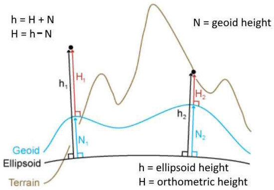
Figure 2.
Above mean sea level (orthometric) height of the point.
Of course, other mathematical systems such as SageMath or Geogebra also enable geographic calculations too. Publication [6] contains the basic mathematical principles of geography. Detailed theoretical information about geodetic coordinate systems can be found in the publication [10], and about plane geometry of the type we use in the design [8].
4.3. Computation of X, Y, and Z Coordinates in the Eci System
The next MATLAB code (version R2022b or higher) calculates coordinates in the Earth-Centred Inertial (ECI) coordinate system (Figure 1). The input data are the GPS coordinates and the altitude (above mean see level height) of the peak of Mount Everest. The outputs are the coordinates of this point in the Euclidean coordinate system with the center at the center of the Earth ((4) point of the algorithm). The calculation requires the Mapping Toolbox of the MATLAB system. This toolbox contains the digital models of the globe (geoid). The results of the computations are given in meters.
This code serves as an example for moving the origin of the coordinate system from the center of the earth to an arbitrary point whose GPS coordinates are known. Here we use the MATLAB command and the digital model of the earth (‘’)) in MATLAB.
- lat = 27.988056;
- lon = 86.925278;
- H = 8848;
- N = egm96geoid(lat,lon);
- h = H + N
- spheroid = referenceEllipsoid(‘GRS 80’);
- [X,Y,Z] = geodetic2ecef(spheroid,lat,lon,h)
- h = 8.8193e+03
- X = 3.0274e+05
- Y = 5.6360e+06
- Z = 2.9795e+06
“Projections for large areas usually use a simple sphere; for smaller areas, where accuracy gains in importance, the projection uses an ellipsoid which locally corresponds to a geoid, the name for the shape with the most accurate correspondence to the actual oblate and irregular shape of the earth at a given time.” [6]. The description of the GRS 80 reference model can be found in the publication [12,13].
4.4. Polygon of the Area of Interest
As stated in the work [17], it is not possible to algorithmically determine a polygon based on significant points of the limited area. Therefore, it is necessary to enter which significant points and in what order will define the polygon that bounds the area of interest. In the mentioned work, it is also stated that a simple polygon can be divided into an upper and a lower part, as we can see in Figure 3. This is the way to obtain the points , which define the polygon of the bounded area.
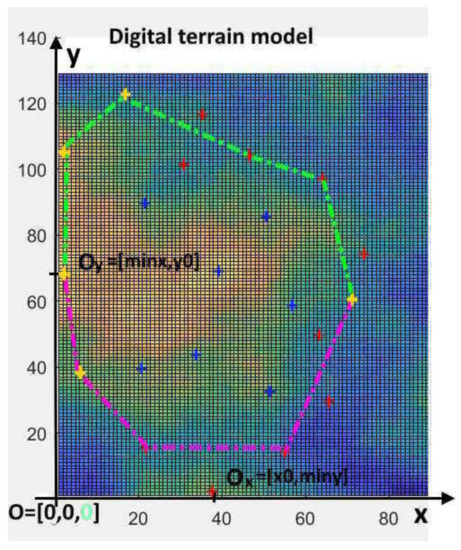
Figure 3.
The area of interest polygon.
Now we need to determine the length of the polygon to be able to estimate the number of sensory units of the network according to relation (2). To calculate the length of the polygon, we need to define the term spatial curve.
Definition 1.
Let be a closed interval. Representation is a spatial curve, is the starting point, is the endpoint of the curve. If then the curve is closed. The curve r is simple, when is a one-to-one correspondence.
The correspondence is one-to-one if each element of the first set is made to correspond with exactly one element of the second set, and vice versa.
Definition 2.
Letbe a spatial curve and is the partition of the interval . The spatial polygon which has vertices , is called an inscribed polygon belonging to partition . The length of the polygon is the sum of the lengths of the edges:
A polygon of an area of interest is a simple, closed spatial curve, which is given by the division of the interval In three-dimensional space, a polygon is given by these points
for Therefore, we can calculate the distances between the points and (see [9,10]) as
The points , from relation (10) define three functions . These functions for our purposes at the moment are not needed, only their functional values in points , so we do not examine the properties of the functions.
4.5. Digital Model of a Area of Interest
We now summarize the procedure for defining a digital model of a area of interest.
The method of defining the area of interest in the terrain model.
| Algorithm 2: Determination of the area of interest in the terrain model. |
|
We note that this method cannot be algorithmized. This is the reason why the application is needed, which with the data inputs and outputs will help solve the area definition problem. When the polygon P is defined, the length of the polygon is calculated based on (9) and according to (2) we can estimate the minimum number of sensory units in the network. The next task will be to create a method to deploy the sensory units on the polygon P.
4.6. Algorithm for Creating a Network of Mobile Sensory Units
Suppose that the polygon P of the area of interest is given. Polygon P contains significant points a . All the necessary significant points that belong to the set are vertices of the polygon P. In a digital model of the terrain is given point . According to this point, the coordinates of the points are given .
| Algorithm 3: Creating a network of sensory units. |
2. , point selection 3. 4. 5. if then (see, point I. on the Figure 4) 6. if then if then (see, point II. on the Figure 4) if then it is possible (there is no obstacle between the points and D) if there is an obstacle between the points and D, then (see, point III. on the Figure 4) 7. if then go to 2 (in this step the polygon with vertices was created) 8. if then , . |
Cases I, II and III from Figure 4 show the procedure for creating a network of sensory units. Coordinates are elements of the matrix A of the digital terrain model (see Figure 3).
Note: Point D lies on the line and at a distance of . Point D is not a significant point.
Brief description of the algorithm: We have a cycle considering the variable j in which we select the vertices of the polygon P. According to points 5–7. we create a polygon . with vertex . Polygons contain a set of necessary significant points and other points where sensory units are located. In point 8, we determine the polygon, which contains the smallest number vertices from that set of polygons .
This method finds a polygon Q such that the length of the polygon is and the number of vertices of Q is less than or equal to the number of vertices of P. The polygon Q is a digital model of the boundary of the area of interest, the vertices of the polygon define the location of the sensor units in the area of interest.

Figure 4.
Selecting the next polygon(network) vertex.
Figure 4.
Selecting the next polygon(network) vertex.

4.7. Data Model of the Network
The coordinate system (coordinate system origin, coordinate system axes), the set of significant points, the polygon of the area of interest and the polygon of the network belong to the mathematical model of the network. We also have other inputs, such as a digital terrain model. This terrain model depends on the detailedness of the terrain d. All these objects need to be defined in the data model of the network.
The raster data model contains the following data structures:
—a table that contains one record in which there are the following items: . The origins of the coordinate system are the actual GPS coordinates, H is its altitude and d is the detailedness of the terrain, which was applied in the creation of a digital terrain model. This information determines the place where the terrain is located in which the network will be set. Values need to be calculated according to relations (4) and (5). Parameters H and d are going to be input parameters. These data define the origin of the coordinate system, it is the reference point of the system and the detailedness of the terrain model, in which resolution we will work.
—table (matrix ) of size —digital terrain model. Digital terrain model can be obtained from existing software such as MATLAB (for detail ) or it is possible to apply special scanners such as LiDAR, where we can achieve a detail of , which means we can divide a 100 cm section into 10 parts, or in other words, the resolution of one table point will be cm.
—a table that contains rows of —set of significant points coordinates in the table , —significant point coding, 1—internal (blue color), 2—necessary boundary (yellow color), 3—borderline (red color in Figure 1 and Figure 3). We note that a suitable choice of significant points helps to define different types of obstacles in the field.
With the help of significant internal points, we can define obstacles as things, events or constructions. Different observation layers can also be created. In that case, matrix A will be three-dimensional. The third dimension can contain layers; for example, the first layer includes the elevation, the second layer structural obstacles and the third layer natural obstacles. In the case of layers, the data complexity of the system grows.
—table (polygon of the area of interest): contains the lines —coordinates of points from the table , which create the polygon of the area of interest.
—table (polygon of the grid): include lines —some coordinates of points and some position data of points.
We can match this basic raster data model to a mathematical model. For completeness, let us note that there may also be a vector data model (see [6]) of the monitored area; but we do not deal with this type of model in this work.
The data model is needed for the next step, for the software implementation of the network modeling application, which can be considered a small geographic information system (GIS). Algorithms applied for GIS systems can be found in the publication [11].
4.8. Steps for Software Implementation
Steps for implementation of the application:
- step of the software implementation is the selection of significant points in the monitored area.
- step is determining the coordinate system (determining the points and ) (with this step, we locate the task).
- step is obtaining a digital terrain model of the monitored area. Determination of input parameters (, , ).This input information is necessary for the application’s software implementation to design the network of sensory units.
- step—the output of the computations are tables of polygons , . is the polygon of the area of interest. is a polygon of sensory units network.
Several solutions are available for the software implementation of a GIS network of sensory elements. One solution is to apply MATLAB v. R2022b and above with the mapping toolbox. This system houses digital models of the globe with functions that enable geographic calculations. Another option is to use the Python programming language. There are extensions for this language, such as ArcGIS, for geographic applications, see [13].
5. Conclusions
The significance of this article is that regardless of the type of sensor units, the proposed methods are applicable to creating a network of sensor units to protect the area of interest. A single input parameter is required for calculation, the communication range of the sensor unit. The practical use of this method will be a program (software implementation of a small geographic information system) with which we can design a network of sensory units. We are currently waiting for the completion and testing of the sensory units. We need primary inputs such as the communication range of the sensory units and determining the terrain of the network location. Our results say that we define the network of sensory units using the polygon of the area of interest. It will also be a polygon, and the vertices of the polygon determine the placement of individual sensory units. These polygons describe a ring topology. In the sensor network, the sensor nodes are the polygon’s vertices.
The work’s main goal was to create a theoretical mathematical and data model of an area of interest and a network of portable sensor units. The considered network of mobile sensor units results from the MOVIR project. In the article, a mathematical model was proposed, which includes the definition of the coordinate system, sets of significant points, and a digital terrain model. With the help of these mathematical objects, we define the model of the area of interest and the network of sensor units, which are a polygon of the area of interest and a sensor unit network polygon. The mathematical model is theoretical, not computational. The data model was designed based on a mathematical model. The model should serve as an input for implementing the geographic information system, a program modeling the area of interest and the digital network of mobile sensory units.
Author Contributions
Conceptualization, P.S. and J.G.; methodology, P.S.; software, J.G. and T.M.; investigation, P.S. and J.G.; resources, J.G.; data collection, T.M.; writing—original draft preparation, P.S. and J.G.; writing—review and editing, P.S.; visualization, P.S. and T.M.; supervision, P.S., J.G. and T.M. All authors have read and agreed to the published version of the manuscript.
Funding
This research was funded by European Regional Development Fund under the Operational Programme Integrated Infrastructure, grant number, ITMS code 313011AUP1.
Institutional Review Board Statement
Not applicable.
Informed Consent Statement
Not applicable.
Data Availability Statement
The data in this work are available from the corresponding authorsupon reasonable request.
Acknowledgments
This work was supported by the project Mobile Monitoring System for the Protection of Isolated and Vulnerable Population Groups against Spread of Viral Diseases, ITMS code 313011AUP1. The authors, gratefully acknowledge European Regional Development Fund under the Operational Programme Integrated Infrastructureand Výskumná agentúra—Research Agency for the technical and financial support.
Conflicts of Interest
The authors declare no conflict of interest.
References
- Buratti, C.; Conti, A.; Dardari, D.; Verdone, R. An Overview on Wireless Sensor Networks Technology and Evolution. Sensors 2009, 9, 6869–6896. [Google Scholar] [CrossRef] [PubMed]
- Stankovic, J.A. Wireless Sensor Networks. Computer 2008, 41, 92–95. [Google Scholar] [CrossRef]
- Yick, J.; Mukherjee, B.; Ghosal, D. Wireless sensor network survey. Comput. Netw. 2008, 52, 2292–2330. [Google Scholar] [CrossRef]
- Kandris, D.; Nakas, C.; Vomvas, D.; Koulouras, G. Applications of Wireless Sensor Networks: An Up-to-Date Survey. Appl. Syst. Innov. 2020, 3, 14. [Google Scholar] [CrossRef]
- Nayak, S.; Zlatanova, S. (Eds.) Remote Sensing and GIS Technologies for Monitoring and Prediction of Disasters; Springer: Berlin/Heidelberg, Germany, 2008. [Google Scholar]
- Harvey, F. A Primer of GIS: Fundamental Geographic and Cartographic Concepts; Guilford Publications: London, UK, 2015. [Google Scholar]
- Maling, D.H. Coordinate Systems and Maps Projections; Pergamon Press: Oxford, UK, 1992. [Google Scholar]
- Chiossi, S.G. Elementary Plane Geometry. In Essential Mathematics for Undergraduates; Springer International Publishing: Berlin/Heidelberg, Germany, 2021; pp. 401–437. [Google Scholar] [CrossRef]
- Sickle, J.V. Basic GIS Coordinates; CRC Press: Boca Raton, FL, USA, 2017. [Google Scholar]
- Lawrence, J.L. Celestial Calculations—A Gentle Introduction to Computational Astronomy; The MIT Press: Cambridge, MA, USA; London, UK, 2018. [Google Scholar]
- Xiao, N. GIS Algorithms; SAGE Publications Ltd.: New Delhi, India, 2015. [Google Scholar]
- Mathworks. Find Ellipsoidal Height from Orthometric Height. Available online: https://www.mathworks.com/help/map/ellipsoid-geoid-and-orthometric-height.html (accessed on 23 April 2023).
- Conley, J. A Geographer’s Guide to Computing Fundamentals; Springer International Publishing: Berlin/Heidelberg, Germany, 2022. [Google Scholar] [CrossRef]
- Kurdel, P.; Češkovič, M.; Gecejová, N.; Labun, J.; Gamec, J. The Method of Evaluation of Radio Altimeter Methodological Error in Laboratory Environment. Sensors 2022, 22, 5394. [Google Scholar] [CrossRef] [PubMed]
- Novotňák, J.; Fiľko, M.; Lipovský, P.; Šmelko, M. Design of the System for Measuring UAV Parameters. Drones 2022, 6, 213. [Google Scholar] [CrossRef]
- Fiľko, M.; Kessler, J.; Semrád, K.; Novotňák, J. Manufacturing of the Positioning Fixtures for the Security Sensors Using 3D Printing. Transp. Res. Procedia 2022, 65, 98–105. [Google Scholar] [CrossRef]
- Szabó, P.; Ferencová, M.; Blišťanová, M. A Spatially Bounded Airspace Axiom. Axioms 2022, 11, 244. [Google Scholar] [CrossRef]
- Kasper, P.; Lipovsky, P.; Smelko, M. Application Software of Modular System for Magnetic Characteristics Measurement. In Proceedings of the 2022 New Trends in Aviation Development (NTAD), Novy Smokovec, Slovakia, 24–25 November 2022. [Google Scholar] [CrossRef]
- Szabó, P.; Ferencová, M.; Železník, V. Cloud Computing in Free Route Airspace Research. Algorithms 2022, 14, 123. [Google Scholar] [CrossRef]


Disclaimer/Publisher’s Note: The statements, opinions and data contained in all publications are solely those of the individual author(s) and contributor(s) and not of MDPI and/or the editor(s). MDPI and/or the editor(s) disclaim responsibility for any injury to people or property resulting from any ideas, methods, instructions or products referred to in the content. |
© 2023 by the authors. Licensee MDPI, Basel, Switzerland. This article is an open access article distributed under the terms and conditions of the Creative Commons Attribution (CC BY) license (https://creativecommons.org/licenses/by/4.0/).