Article

Cloud–Edge Hybrid Computing Architecture for Large-Scale Scientific Facilities Augmented with an Intelligent Scheduling System

1
Shanghai Synchrotron Radiation Facility, Shanghai Advanced Research Institute, Chinese Academy of Sciences, Shanghai 201210, China
2
Shanghai Institute of Applied Physics, Chinese Academy of Sciences, Shanghai 201204, China
3
School of Physical Science and Technology, ShanghaiTech University, Shanghai 201210, China
*
Authors to whom correspondence should be addressed.
Appl. Sci. 2023, 13(9), 5387; https://doi.org/10.3390/app13095387
Submission received: 9 April 2023 / Revised: 24 April 2023 / Accepted: 24 April 2023 / Published: 26 April 2023

Abstract

:
Synchrotron radiation sources are widely used in interdisciplinary research, generating an enormous amount of data while posing serious challenges to the storage, processing, and analysis capabilities of the large-scale scientific facilities worldwide. A flexible and scalable computing architecture, suitable for complex application scenarios, combined with efficient and intelligent scheduling strategies, plays a key role in addressing these issues. In this work, we present a novel cloud–edge hybrid intelligent system (CEHIS), which was architected, developed, and deployed by the Big Data Science Center (BDSC) at the Shanghai Synchrotron Radiation Facility (SSRF) and meets the computational needs of the large-scale scientific facilities. Our methodical simulations demonstrate that the CEHIS is more efficient and performs better than the cloud-based model. Here, we have applied a deep reinforcement learning approach to the task scheduling system, finding that it effectively reduces the total time required for the task completion. Our findings prove that the cloud–edge hybrid intelligent architectures are a viable solution to address the requirements and conditions of the modern synchrotron radiation facilities, further enhancing their data processing and analysis capabilities.

1. Introduction

In recent years, the rapid development of the large-scale synchrotron radiation facilities has brought the electron beam divergence close to the diffraction limit, while steadily increasing both the photon flux and coherence. As the experimental techniques at the new generation light source facilities are evolving in order to match modern users’ needs in terms of high-throughput, multimodal, ultrafast, in situ, and dynamic investigations, this lays the foundation for real-time, multi-functional, and cross-facilities experiments. In addition, the imaging sensors, such as the complementary metal oxide semiconductor (CMOS) and charge-coupled device (CCD), have made remarkable advancements in terms of smaller pixel sizes, larger areas, and faster frame rates, allowing for experimental techniques with a better spatial and temporal resolution. Their widespread usage in beamlines has gradually caused the digital images to become the predominant scientific raw data format in synchrotron radiation facilities [1]. As a result, within the next few years, the resulting exponential increase in terms of data volume will exceed the processing capability of the existing classical methods relying on manned data analysis. This “data deluge” effect [2] has severely challenged all the synchrotron radiation facilities worldwide, particularly in terms of data acquisition, local storage, data migration, data management, data analysis, and interpretation.
For example, the X-ray photon correlation spectroscopy can now generate images with a file size of 2 MB at 3000 Hz with a data generation rate of 6 GB/s [3], which is comparable to the data rate of the Large Hadron Collider. Using the Oryx detector, tomography beamlines can acquire 1500 projections of 9 s each (with each consisting of 2048 × 2448 pixels) at a data rate exceeding 1 GB/s [4]. Using these techniques, it is possible to study time-dependent phenomena for several weeks, accumulating an enormous amount of data. According to the statistics from the National Synchrotron Light Source-II (NSLS-II) [5,6], solely in 2021, over 1 PB of raw data was generated, and the future data volumes are expected to further increase. Furthermore, it is expected that the High Energy Photon Source (HEPS) under development in China will generate, with its 14 beamlines, 24 PB of raw experimental data per month during the initial phase [7].
Therefore, due to the vast amount of data generated during these experiments, novel capabilities in terms of on-site real-time data analysis, processing, and interpretation at the beamlines are a crucial and urgent need for the synchrotron radiation users. Not addressing this issues may then result in a large portion of the users’ data not being effectively analyzed, obscuring any potential scientific discovery hidden within these data [8].

1.1. Classical Approaches at the Synchrotron Radiation Facilites

Synchrotron beamlines typically offer two approaches to provide users with on-site data processing and analysis services to address their computationally intensive needs. The first approach involves uploading data and jobs to a national supercomputer via high-speed scientific network infrastructures. The second approach involves the deployment of on-premises high-performance workstations, or small clusters, dealing with the task involving the data processing jobs.
For example, the Superfacility project [9] at the Lawrence Berkeley National Laboratory (LBNL) links research facilities with the National Energy Research Scientific Computing Center (NERSC)’s high-performance computing (HPC) resources via ESnet [10], allowing for large-scale data analysis with minimal human intervention. This decreases the length of the analysis cycles from days or weeks down to minutes or hours. Users have the possibility of accessing storage, open software, and tools without the need of managing complex architectures or possessing computational competences [11,12,13,14]. The Advanced Light Source (ALS) has launched several projects at the NERSC, including a data portal, a data-sharing service, and an artificial intelligence (AI)/machine learning (ML) collaboration project, streamlining for the users the data ingestion, sharing and labeling processes [15]. This approach adheres to the concept of resource concentration and intensification. However, it is important to note that the resource allocation and scheduling, as well as the queuing time, are beyond the control of the beamline scientists and users, due to the operational regulations of the supercomputer itself. Taking the example of the ALS using the SPOT framework and NERSC to process tomography data, the actual job execution time for computed tomography (CT) reconstructions was less than 10 min, while the queuing time in the NERSC scheduling system was circa 30 min [15].
The TOMCAT beamline, at Swiss Light Source, has instead adopted an on-premises computing system approach, installing the GigaFRoST detector system for quick data acquisition [16] and creating an effective tomographic reconstruction pipeline using high-performance computing to manage and analyze the massive data influx [17,18]. The TomoPy framework [19], developed by the Advanced Photon Source (APS) using Python, represents a highly effective data-intensive strategy. ALS has adopted and further developed the TomoPy framework by implementing a modernized user interface [20], which can considerably increase the CT users’ workflow efficiency. Until 2019, the macromolecular crystallography (MX) beamlines at the SSRF utilized an automated system, Aquarium [21], which employed a local dedicated high-performance computing cluster for large-scale parallel computations. This expedites the data reduction, single-wavelength anomalous diffraction (SAD) phasing, and model construction procedures, which took place within a 5 to 10 min time window. Although local dedicated small-scale computing clusters can ensure real-time job execution through resource exclusivity, they come with the limits of higher economic costs and a lower scalability.
Integrating the two approaches could then result in a more efficient solution that prioritizes the usage of local dedicated infrastructures matching the real-time needs of the users’ experiments, and then allocates computational tasks to large computing centers when higher computational demands arise, all within a framework designed to accommodate the needs of the diverse scientific communities. This hybrid approach will provide substantial benefits but requires close collaboration between the local computing infrastructures at the beamlines and the large computing centers in order to ensure a seamless integration and an efficient data transfer.

1.2. Shanghai Synchrotron Radiation Facility (SSRF)

The SSRF is the first medium-energy, third-generation synchrotron radiation source on the Chinese mainland. It features a 150 MeV linear accelerator, a 3.5 GeV booster, a 3.5 GeV storage ring, 27 operational beamlines, approximately 40 operational experimental endstations, support facilities, and a dedicated data center [22,23,24,25,26,27]. With the ongoing development of the SSRF, and the expansion of its application scope, the amount of data generated exhibits a similar upward trend, including varying computing requirements for various beamlines, as shown in Appendix A Table A1.
In 2019, the SSRF generated over 0.8 PB of unprocessed data and 2.4 PB of processed data. Once the Phase II project is completed, the SSRF is expected to generate approximately 30 PB of raw data and 100 PB of processed data per year. Assuming a dataset size of 10 GB, on average, the SSRF can currently process one dataset every 3 min. If the daily volume of data processed reaches 160 TB and totals 16,384 datasets, it would take 819 h to complete a single day of computing tasks [25].
In this context, the processing and analysis of the data from the large-scale synchrotron radiation sources, as well as the improvement of the computing resource usability and data transfer efficiency, are subject to intensive research. As an emerging computing paradigm, edge computing [28,29] relocates the computing resources and data processing capabilities to the network edge, thereby addressing latency, bandwidth bottlenecks, and other challenges inherent to the conventional computing models. Thus, it has the potential for being an effective data processing and analysis solution for the synchrotron radiation facilities [30,31].
With this article, we propose a cloud–edge hybrid intelligent system design scheme tailored to the SSRF’s specific conditions and requirements, in order to improve the efficacy and reliability of the data processing and analysis.

2. Materials and Methods

As a large-scale scientific facility, the SSRF operates around-the-clock to assist users in undertaking a variety of scientific investigations. Due to the intricacy and time-consuming nature of the experimental designs, the lengthy project application processes, and the high cost of a beam time, it is impractical to test novel computing architectures using real-world experiments. To validate the performance and reliability of the new computational architecture, this study employs a simulation-based experimental methodology, simulating the computational tasks, resources, and scheduling processes of the SSRF. This technique decreases the expense and risk associated with performing experiments in a production environment, laying the theoretical groundwork for the SSRF’s future implementation of cloud–edge hybrid intelligent systems.

2.1. Architecture Design of the Cloud–Edge Hybrid Intelligent System (CEHIS)

2.1.1. Computing Infrastructure

The Big Data Science Center (BDSC) at the SSRF is an important infrastructural project of the SSRF Phase II, which is tasked with centralizing, unifying, managing, curating, and formatting all the data generated by all the SSRF beamlines, while providing real-time data analysis capabilities to the users. As shown in Table 1 and Table 2, the HPC Cluster Computing System I was initially configured in 2019 when the Big Data Science Center started its commissioning and operations, while the HPC Cluster Computing System II was subsequently added to it in 2021, after carefully evaluating its operational status for about one and a half years, in order to expand its resources. In total, the BDSC now has 208 CPU nodes, 9 GPU nodes, 3 fat nodes, nearly 11,000 CPU cores, and 28 GPU cards, with a total theoretical peak computing power of 967.8 TFLOPS.
In 2021, the BDSC expansion project not only increased the computing power of the HPC cluster systems, but also deployed 19 edge systems on-premises at the SSRF beamlines. These edge systems have been flexibly configured in order to meet the asymmetric computing resources and storage requirements. Table 3 provides details on the 19 edge systems.
This has provided the SSRF with an effective computing infrastructure, capable of supporting a modern cloud–edge hybrid computing architecture, as shown in Figure 1.

2.1.2. Modeling

In the simulation experiment, we model a computational node within the CEHIS as a one-dimensional vector [ n o d e _ i d , n o d e _ t y p e , c p u , m e m o r y , s t o r a g e ]. The node_id is the unique identifier for the node. The n o d e _ t y p e denotes the type of node, which is either an edge-based node (edge) or a cloud-based node (cloud). The c p u represents the computational resources allocated to the node, while m e m o r y indicates the memory resources provided to the node, and s t o r a g e signifies the storage resources available to the node. If a task is assigned to an edge node, it can be executed immediately; if it is allocated to a cloud-based node, it requires a certain amount of time before it can be executed, accounting for delay introduced by the transmission time.

2.1.3. Pipelines

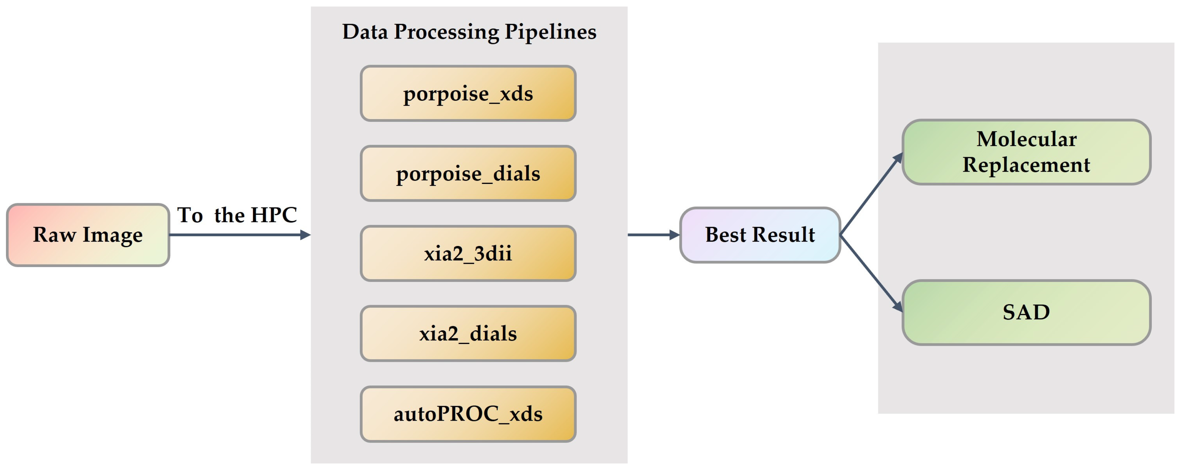
Scientific computation approaches, such as the matrix multiplication and solving systems of linear equations, are essential components of the SSRF’s computational activities. These computations often involve the management of massive amounts of data and rely on parallel and distributed computing in order to enhance the data processing performance. For instance, after acquiring a dataset using the Aquarium system, the automated data analysis system at the SSRF MX beamline launches five HPC parallel pipelines concurrently. These pipelines apply a variety of data reduction techniques, and the best result from the five pipelines is then selected for further processing. Therefore, a single job sent by the Aquarium to the data center consists of five tasks with different degrees of complexity and execution time. The entire data processing workflow of the Aquarium system is illustrated in Figure 2.
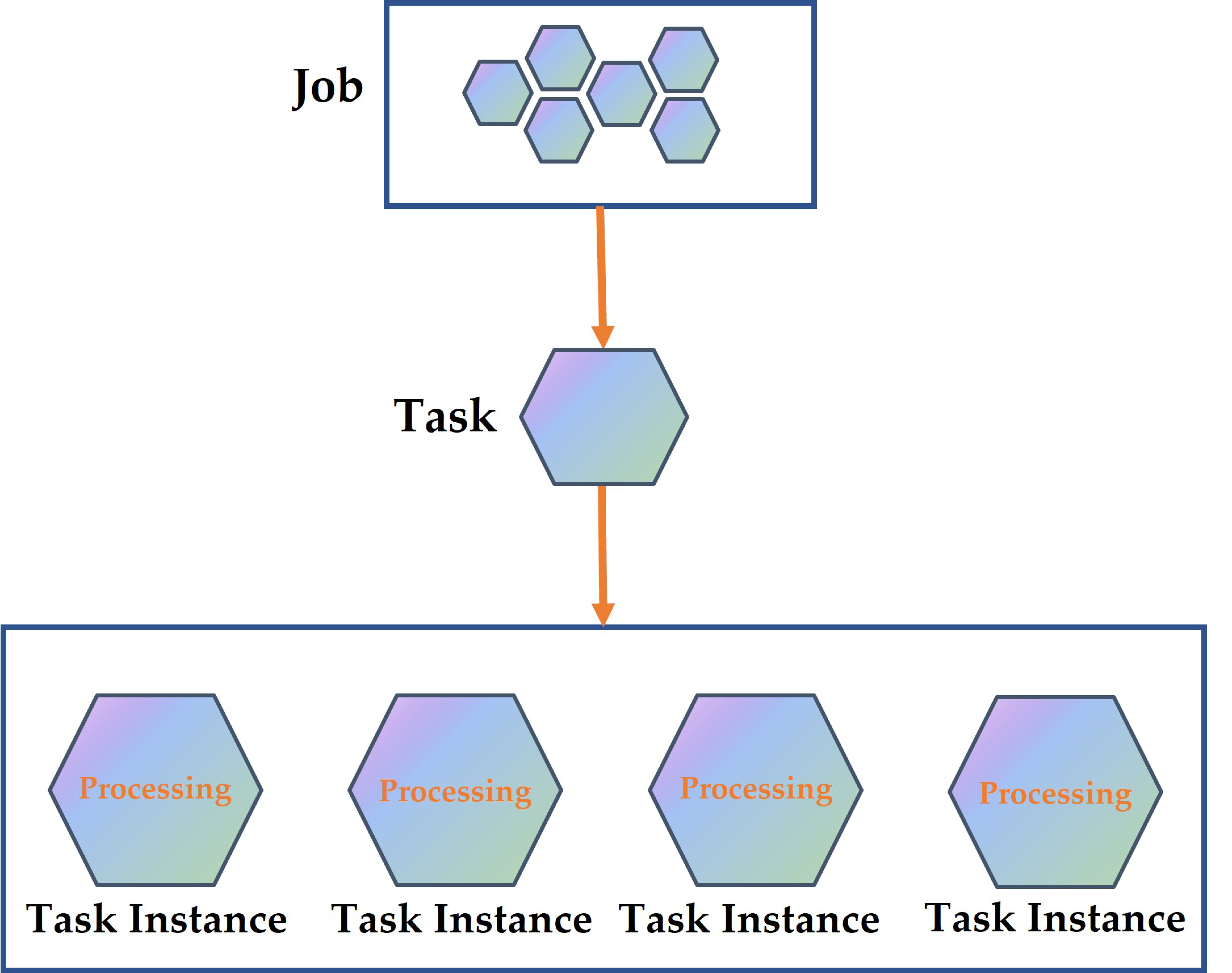
With our study, we have simulated the queuing jobs and tasks generated by the beamlines at the SSRF, where the computational tasks submitted by the users are modeled as jobs, with each job consisting of several tasks and scheduling being performed at the task level. A task is represented by [ s u b m i t _ t i m e , d u r a t i o n , c p u , m e m o r y , j o b _ i d , t a s k _ i d , i n s t a n c e _ n u m ] . The t a s k _ i d is the unique identifier for the task, whereas j o b _ i d identifies the job to which the task belongs. The s u b m i t _ t i m e specifies the time at which the task was submitted, whereas d u r a t i o n indicates the time required to run a single task instance. The c p u represents the computing resources necessary for the task, while m e m o r y signifies the memory resources necessary for the task, and i n s t a n c e _ n u m indicates the number of task instances. A variable number of task instances can be defined for each task, based on the analysis of the SSRF’s computational requirements and task characteristics, as previously described. In contrast, a task instance is an individual execution instance of a task. When a task is repeated several times, either in parallel or with different input parameters, each of these executions is referred to as a task instance. The task instance is effectively a running instance of the task, and it is the task instance that is scheduled and executed on a computing node. A computational job and its structure are shown in Figure 3.

2.1.4. Service Delivery Paradigm

The CEHIS service delivery paradigm is shown in Figure 4. N o d e s = [ C l o u d _ 1 , C l o u d _ 2 , C l o u d _ 3 , , C l o u d _ h , E d g e _ 1 , E d g e _ 2 , E d g e _ 3 , , E d g e _ k ] represents the overall computational resources of the CEHIS, which consist of the cloud-based high-performance computing clusters and edge computing systems. During user experiments, the data acquisition system or users manually submit computational jobs J o b s = [ J _ 1 , J _ 2 , J _ 3 , , J _ m ] to the intelligent scheduling system. After these job tasks enter a queue pool, the scheduler assigns a computational node to each task, based on a predetermined strategy. The assigned computational node could be an edge node “ E d g e _ i ” or a node within the cloud-based high-performance computing cluster “ C l o u d _ j ”. Theoretically, edge nodes are appropriate for real-time computational tasks, whereas cloud nodes are optimal for workloads with large computational demands and no real-time requirements.

2.2. Task Scheduling Algorithm

Task scheduling includes assigning a set of pending tasks to a group of computing nodes in specific accordance with user specifications. The objective of the task scheduling for the CEHIS is to reduce the task completion time as much as possible, hence, enhancing the system performances and resource utilization. Selecting a suitable scheduling algorithm is the key factor in order to achieve the main objective of task scheduling.

2.2.1. Classical Scheduling Algorithms

The random scheduling (RS) method iterates through all the viable task and machine combinations and creates a tuple for each combination. The algorithm then determines, for each possible combination, which combination to select, based on a randomly generated value and a threshold. The combination is selected if the randomly generated value is larger than the threshold; otherwise, the loop continues, and another combination is sought. If there are no possible task and node combinations, the algorithm yields none. The objective of this technique is to schedule tasks efficiently by satisfying node capacities and task requirements while selecting tasks and nodes randomly.
First Fit (FF) is an algorithm designed to assign tasks sequentially to the first available node that fits their requirements. Specifically, at the start of the scheduling procedure, the FF algorithm iterates through all task and node combinations in search of a node that fits the requirements and is available. After locating a suitable node, the algorithm assigns the task to it and removes it from the task list. If there are no available nodes, the task remains in the task list until an appropriate node becomes available.
The Tetris packing algorithm is named after the popular video game Tetris because it places tasks into nodes by stacking blocks in accordance with certain principles. The Tetris algorithm computes the fitness between all the viable nodes and tasks, then selects the node–task combination with the highest fitness. The evaluation criteria for the fitness computation is the product of the resource utilization rates of the node and task; the greater the fitness, the more balanced the resource utilization between the node and task. This method of selection enables the Tetris algorithm to prevent fragmentation of residual capacity to a certain degree, resulting in a higher utilization rate.
Classical scheduling methods, such as the aforementioned RS, FF, and Tetris algorithms, can partially serve the scheduling needs of computational tasks. However, they have two constraints, as listed below:
  • Lack of adaptability. Classical scheduling algorithms are often inflexible, meaning that once a task has been scheduled on a machine, it cannot be rescheduled. In real-world applications, however, task characteristics may change with time and environmental conditions, demanding ongoing modifications and optimizations of the task scheduling systems.
  • Lack of optimization. Traditional scheduling algorithms are frequently dependent on heuristic principles or greedy strategies, making it difficult to identify the globally best solution. In addition, due to the interactions between activities, simple task scheduling is frequently insufficient to address the optimization needs of the system.

2.2.2. Deep Reinforcement Learning

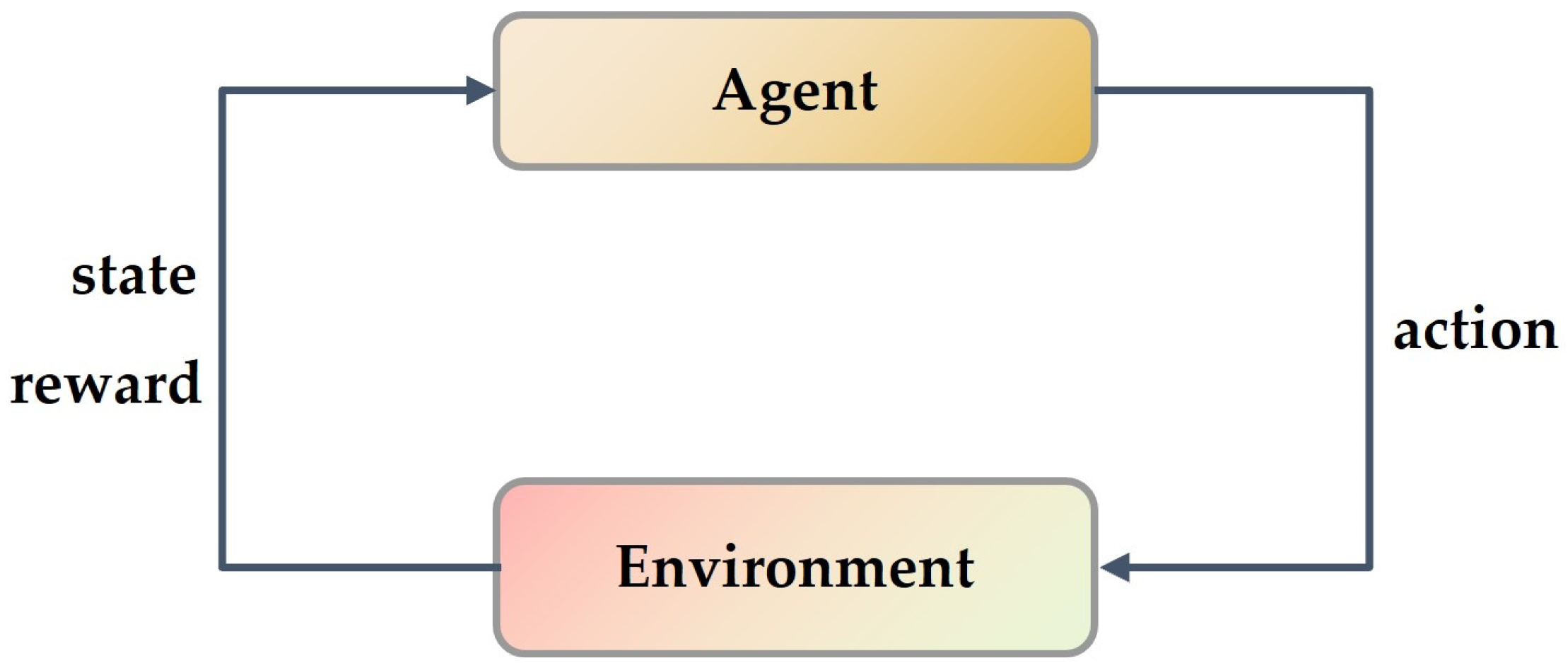
Reinforcement learning (RL) [32], as shown in Figure 5, is a subfield of machine learning that enables intelligent agents to learn the optimal action policy by interacting with their environment. In RL (Figure 5) the agent obtains the state information S t and reward R t from the environment and selects an action A t according to its policy. In response to the agent’s action, the environment offers feedback R t + 1 , which is used to modify the agent’s policy, allowing it to better adapt to the environment. Policy, reward, value, and environment are the four key components that the RL includes. Specifically, the policy describes the agent’s behavior in response to a particular state, the reward defines immediate feedback, and the value defines the long-term gain.
In RL, as opposed to supervised learning, there are no labeled training data. The agent can only acquire knowledge by interacting with the environment. This provides RL with a substantial edge in numerous practical applications, such as autonomous driving, robot control, and game design.
Deep reinforcement learning (DRL) combines RL and deep learning (DL) by employing deep neural networks (such as the convolutional neural networks, CNNs) to estimate the agent’s policy or value functions, hence, allowing the learning of more sophisticated action policies. DRL algorithms can also be used to train agents to learn task scheduling policies, adaptively change the task scheduling strategies, optimize scheduling rewards, and provide a degree of flexibility and real-time responsiveness. Consequently, DRL algorithms are a potentially effective method for task scheduling.

2.3. Policy Gradient-Based Deep Reinforcement Learning

Policy gradient methods are a category of model-free reinforcement learning algorithms that directly optimize the policy parameters, rather than estimating the value functions [33]. The fundamental concept underlying the policy gradient methods is to update the policy along the expected reward gradient about the policy parameters. This gradient-based optimization procedure enables the agent to discover superior policies by utilizing the structure of the problem, while retaining the adaptability to respond to changes occurring within the environments. The CEHIS task scheduling process, with a policy gradient-based DRL algorithm, is shown in Figure 6.

2.3.1. Policy Network

A policy function, frequently symbolized with π , is a central concept in RL that specifies the decision-making strategy of an agent in a given environment. The agent chooses an action for a given state based on the probability distribution described by the policy. Mathematically, a policy can be expressed as a mapping function π : S P ( A ) , where P ( A ) is the probability distribution over the action space A , and S is the state space.
CNNs can be used as function approximators to represent the policy of an agent by mapping the observed state to a probability distribution across actions. The policy network can be expressed as π ( a | s , θ ) , where a denotes an action, s denotes a state, θ denotes trainable neural network parameters, and a A π ( a | s , θ ) = 1 .
As shown in Figure 7, a CNN-based policy extracts features from the raw input, including the status of the pending jobs and available computing resources, using a succession of convolutional layers. Afterwards, the convolutional layers, with typically one or more fully connected layers, are employed to integrate the retrieved features and capture higher-level abstractions, resulting in a dense representation of the input.
The final layer of the CNN-based policy is a softmax activation layer that converts the dense representation into an action space probability distribution. The softmax function guarantees that the output probabilities are non-negative and accumulate to one, allowing them to be interpreted as action probabilities. The agent then samples an action from this distribution to instruct the scheduler on how to choose a node for the waiting tasks.

2.3.2. Policy Gradient

Let us consider a reinforcement learning problem with a policy π ( a | s , θ ) , where π represents a probability distribution over actions a , given state s , and θ denotes the policy parameters. The objective function we aim to maximize is the expected cumulative reward, which can be expressed as follows:
J θ = E t = 0 T γ t R t | π
where γ is the discount factor, R t is the reward at timestep t , and T is the time horizon.
To maximize the J θ , we need to find the gradient of the objective function with respect to the policy parameters θ . Using the likelihood ratio trick, we can rewrite the gradient as follows:
J θ = J θ θ = E t = 0 T l o g π ( a t | s t , θ ) θ γ t R t
The expectation is the above formula that can be estimated using Monte Carlo sampling. By collecting a set of trajectories τ = [ a 0 , s 0 , a 1 , s 1 , , a T , s T ] using the current policy π , we can approximate the expectation as follows:
J θ 1 N i = 1 N t = 0 T l o g π ( a t i | s t i , θ ) θ γ t R t i
where N is the number of trajectories sampled, and ( a t i , s t i , R t i ) represents the state, action, and reward at timestep t in the i -th trajectory.
This approximation is unbiased because the expectation of the Monte Carlo estimate is equal to the true gradient. In other words, as the number of the sampled trajectories N approaches infinity, the estimate converges to the actual policy gradient, as follows:
E J θ θ = J θ θ
In conclusion, the policy gradient method optimizes the policy parameters by computing the gradient of the expected cumulative reward with respect to the policy parameters. Monte Carlo sampling is employed to estimate the gradient, providing an unbiased estimate of the true gradient as the number of sampled trajectories increases.

2.3.3. Advantage Function and Baseline

The advantage function, denoted as A ( s , a ) , is a crucial concept in reinforcement learning that measures the relative value of taking a specific action in a given state compared to the average value of actions in that state. Therefore, the advantage function measures how much better or worse an action is compared to the average action in the same state according to the policy. Mathematically, the advantage function is defined as the difference between the action value function Q ( s , a ) and the state value function V ( s ) , as follows:
A s , a = Q s , a V s
A baseline is introduced to further decrease the variance in the policy gradient estimation without affecting the expected gradient. A baseline is a function, b ( s ) , that estimates the expected value of the advantage function for a given state. In practice, the state value function V ( s ) is often used as a baseline. By subtracting the baseline from the estimated Q-values, the resulting advantage values used in the policy gradient updates have reduced variance. This is because the difference between the Q-value and the baseline captures the relative importance of an action in a particular state, making the gradient estimation more focused on the action preference, rather than the absolute value.
Importantly, introducing a baseline does not affect the expected value of the gradient. Consider the policy gradient theorem, as follows:
J θ = J θ θ = E τ t = 0 T l o g π ( a t | s t , θ ) θ Q π s t , a t
Q π s t , a t = A π s t , a t + V π s
J θ = J θ θ = E τ t = 0 T l o g π ( a t | s t , θ ) θ A π s t , a t + V π s
When a baseline b(s) is subtracted from the Q-value, the new advantage estimate becomes Q ( s , a ) b ( s ) . If b s = V ( s ) , the expected value of the gradient is now given by the following:
E τ t = 0 T l o g π ( a t | s t , θ ) θ A π s t , a t = 0
Therefore, adding or subtracting a baseline does not change the expected gradient, but it significantly reduces the variance, thus, leading to more efficient learning.

2.3.4. Reward-to-Go Method

In the “reward-to-go” policy gradient approach, the concept revolves around the estimation of the Q-values by considering the cumulative rewards starting from the current timestep. The central idea behind this method is to emphasize the contribution of future rewards in the Q-value estimation, thus, allowing the agent to focus on the long-term impact of its actions.
Let Q π ( s t , a t ) represent the expected cumulative reward following the policy π after taking action a t at state s t , as follows:
Q π s t , a t = E t = t T γ t t r ( s t , a t ) | s t , a t , π
where γ is the discount factor, r s t , a t represents the reward at timestep t , and T is the final timestep.
In the “reward-to-go” policy gradient method, we estimate Q π s t , a t using the discounted sum of rewards starting from timestep t, as follows:
Q t = t = t T γ t t r s t , a t
In contrast, the standard policy gradient method typically uses the total discounted reward for the entire trajectory to compute Q-values, which may not fully capture the long-term consequences of individual actions. The “reward-to-go” method offers advantages over conventional policy gradient approaches, encouraging the agent to select actions that not only yield immediate rewards but also maximize long-term gains. Additionally, the “reward-to-go” method is more sensitive to the temporal structure of the problem, potentially leading to faster convergence and better performances.

3. Results

3.1. Computing Architecture

The CEHIS and a cloud computing (CC) system are hereby simulated. The CEHIS comprises cloud nodes and edge nodes, representing the upgraded computing resources of the SSRF. In contrast, the CC system includes only high-performance cloud nodes, representing the computing resources of the SSRF without the edge service system configuration. In order to simulate the SSRF’s computing resources as realistically as possible, we set the computing power of the cloud nodes to be 10 times that of the edge node and the memory of the cloud nodes to be 4 times that of the edge nodes. We use the RS algorithm, FF algorithm, and Tetris algorithm to schedule task sequences of different sizes, and we evaluate the performances using multiple metrics, including the makespan, simulation time (ST), average completion time (ACT), and average slowdown (ASD).
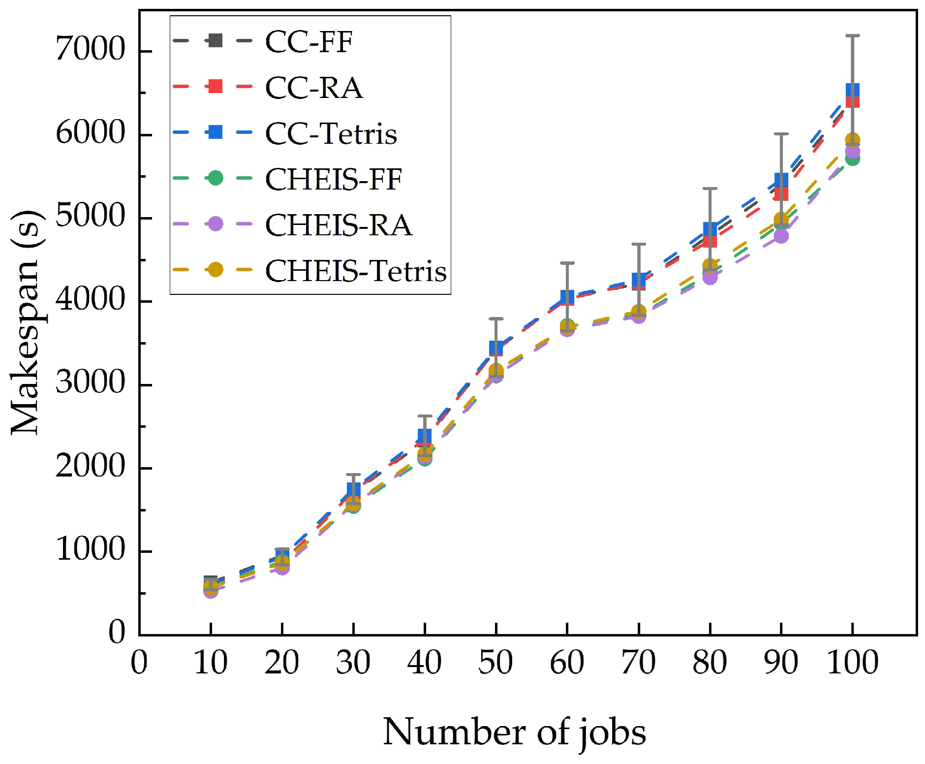
The makespan refers to the time required to accomplish all the tasks, i.e., the duration from the submission of the first task to the completion of the last task. The shorter the makespan of a scheduling algorithm, the more efficient it is. Figure 8 shows that the system architecture has a significant impact on the makespan. The makespan in the CEHIS is much smaller than that in the CC systems. The reason for this is that the CEHIS includes both the edge nodes adjacent to the users, which can reduce transmission time, and the high-performance cloud nodes located further away from the users. Compared to the CC system, the makespan of the CEHIS is reduced by circa 10%.
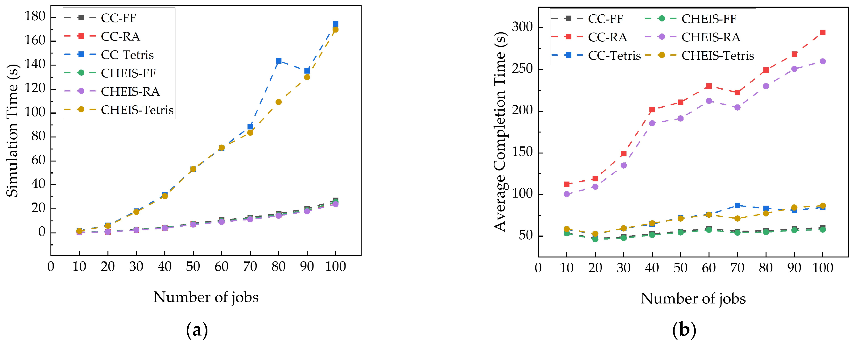
ST is used primarily to measure the time complexity of an algorithm. It tracks the duration from the start of the simulation to the end. Unlike the other three metrics, ST records the computer system time rather than that of the simulation system. Suppose that there are N tasks and M nodes in the system; at each timestep, the RS algorithm must explore all tasks and all nodes to determine if a match is possible. The task–node pair is added to a candidate sequence if a match is discovered. Simultaneously, after each check, a random number is generated, and if the random number is less than a threshold, a random match from the candidate sequence is selected, and the loop is exited. Therefore, the best-case time complexity of the RS algorithm is O ( 1 ) , and the worst-case time complexity is O ( M N ) . The time complexity of the FF algorithm is similar to that of the RS algorithm.
The Tetris algorithm is based on a greedy strategy, requiring the calculation of compatibility between all the tasks and all the nodes, and then sorting all task–node pairs by compatibility, selecting the most compatible match. The time complexity of calculating compatibility is O(NM), sorting is O ( N l o g N ) , and selecting the best match is O ( 1 ) . Thus, Tetris has a temporal complexity of O ( N M + N l o g N ) . As shown in the graph below, the simulation time of the Tetris algorithm is much longer than the other two algorithms.
Let S a T denote the start time of a task and F T denote the finish time of the task. Then, the average completion time of all tasks is as follows:
A C T = 1 N F T i S a T i N
Figure 9 shows that the Tetris algorithm has a much higher simulation time than the RA and FF algorithms due to its high time complexity. On the other hand, the randomness within the RA algorithm may result in the allocation of a task with a small computational requirement to a powerful node, leading to resource wastage and indirectly affecting the overall efficiency of the computing system.
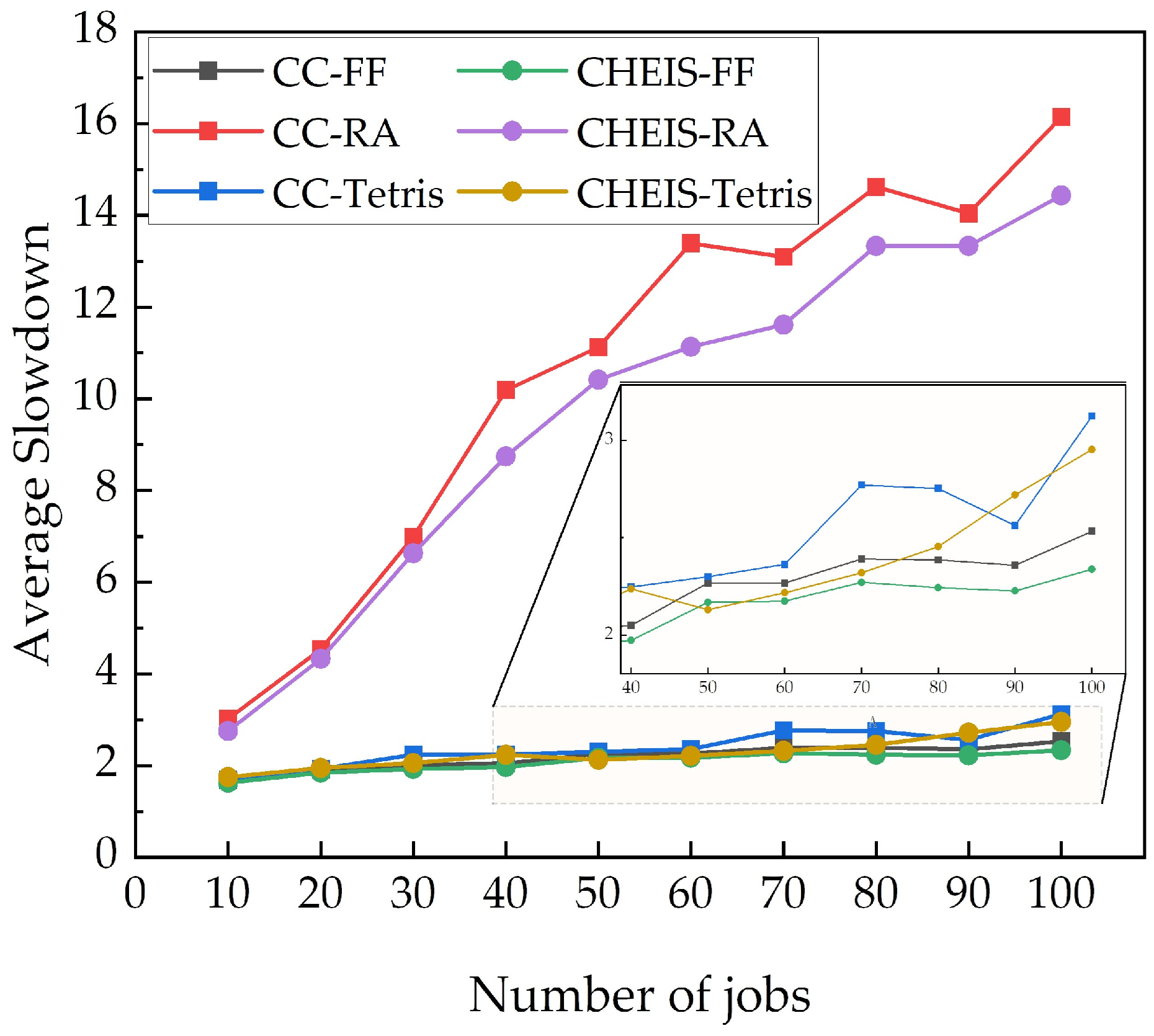
The task slowdown is the ratio of the completion time and the execution duration. The average slowdown of all the tasks is as follows:
A S D = 1 N F T i S a T i d u r a t i o n i N
Figure 10 shows the slowdown of different task scheduling algorithms in the CEHIS and CC systems. A smaller slowdown indicates less time spent in waiting and scheduling processes, resulting in a higher system efficiency. Due to its randomness, the RA algorithm performs poorly on this metric, while the FF algorithm performs the best. Furthermore, we can observe that the slowdown in the CEHIS is generally better than that in the CC system.
This comparison highlights the advantages of utilizing the CEHIS for data processing and analysis in synchrotron radiation facilities, such as the SSRF. The combination of an efficient task scheduling algorithm, such as the FF algorithm, with the CEHIS can lead to an improved system efficiency, while reducing the waiting times, ultimately enabling a more effective use of the computing resources in these facilities.

3.2. Inteligent Task Scheduler

In the experiment, 10 edge nodes and 5 cloud nodes were chosen as computing resources, and their performances were evaluated using 30 and 50 jobs, respectively. To optimize makespan, the policy gradient-based DRL algorithm was compared with the RS, FF, and Tetris algorithms. Table 4 and Table 5 show the results for each metric. By comparing the experimental findings, it was determined that the makespan was lowered by approximately 5% in the case of 30 jobs, and 5% to 12% in the case of 50 jobs. This demonstrates that DRL may optimize makespan and enhance the system efficiency. In addition, the DRL algorithm combines the advantages of the RA, FF, and Tetris algorithms, without compromising the other performance metrics, while optimizing makespan. However, due to the intricacy of the procedure, the computer simulation time is relatively longer.

4. Discussion and Conclusions

In this work, we focused on the key findings and implications of our study on optimizing data processing and analysis for the synchrotron radiation facilities, with a particular emphasis on two critical aspects: the computing architecture and the intelligent task scheduling.
Our proposed CEHIS significantly improves the makespan over the CC approach, resulting in an ideal solution for the large-scale scientific facilities, such as the SSRF. The performances of different scheduling algorithms (RS, FF, and Tetris) highlight the importance of selecting the appropriate algorithms based on the job workload and the computational demands. The policy gradient-based DRL algorithm effectively optimizes the makespan and the system efficiency without compromising other performance metrics. However, its complexity and demanding simulation time require further investigation to broaden its applicability.
In conclusion, the CEHIS, equipped with the intelligent task scheduler, positively impacted the SSRF, and particularly resulted in the following:
  • Improved efficiency. The shorter makespan suggests that the CEHIS can process and analyze data more efficiently, enabling faster completion of the experiments and the analysis tasks.
  • Enhanced resource utilization. The CEHIS allows for more effective allocation and utilization of computing resources, thereby reducing the resource wastage and the overall costs.
  • Better real-time responsiveness. With edge nodes located closer to the data sources, the CEHIS can provide faster response times and lower latency, successfully satisfying the real-time requirements of the SSRF beamlines.
  • Scalability. The CEHIS offers a more scalable solution, as it can flexibly allocate resources between the cloud and edge nodes, making it better suited to handle the future increasing data volumes and computational demands.
  • Encouraging interdisciplinary research. The improved efficiency and responsiveness introduced by the CEHIS can facilitate collaborations across different research fields, fostering innovation and scientific discovery.
Our findings offer vital insights into the optimization of the data processing and analysis infrastructure at the large-scale scientific facilities, laying the groundwork for the development and deployment of the cloud–edge hybrid architectures and intelligent scheduling algorithms.

Author Contributions

Conceptualization, A.S., C.W. and R.T.; methodology, J.Y., C.W. and A.S.; software, J.Y., J.C. and A.S.; validation, R.W., C.W. and X.L.; formal analysis, J.Y. and C.W.; investigation, J.Y. and C.W.; resources, A.S., R.W. and X.L.; data curation, J.C. and R.W.; writing—original draft preparation, J.Y., C.W. and A.S.; writing—review and editing, A.S. and R.T.; visualization, A.S. and R.T.; supervision, A.S., C.W. and R.T.; project administration, A.S. and R.T.; funding acquisition, A.S., C.W. and R.T. All authors have read and agreed to the published version of the manuscript.

Funding

This research was funded by the Photon Science Research Center for Carbon Dioxide, CAS, the Youth Innovation Promotion Association, CAS (Grant no. 2022290), and the Natural Science Foundation of Shanghai (Grant no. 19ZR1463200).

Institutional Review Board Statement

Not applicable.

Informed Consent Statement

Not applicable.

Data Availability Statement

Data is available on request to the authors.

Acknowledgments

We acknowledge support from the Shanghai Synchrotron Radiation Facility (SSRF), Shanghai Advanced Research Institute (SARI), and Chinese Academy of Sciences through the Big Data Science Center (BDSC) project.

Conflicts of Interest

The authors declare no conflict of interest.

Appendix A

Table A1. Data volume of the SSRF Phase Ⅱ Beamlines.
BeamlineArea of ApplicationAverage Output
(Byte/Day)
Max Burst
(Byte/Day)
BL20U1/U2Energy material (E-line)300 MB500 MB
BL11BHard X-ray spectroscopy300 MB500 MB
BL16U1Medium-energy spectroscopy300 MB500 MB
BL07USpatial-resolved and spin-resolved angle resolved photoemission spectroscopy and magnetism (S2-line)300 MB500 MB
Resonant inelastic X-ray scattering300 MB500 MB
BL02U1Membrane protein crystallography12 TB20 TB
BL02U2Surface diffraction12 TB20 TB
BL03SBLaue micro-diffraction7.5 TB15 TB
BL13UHard X-ray nanoprobe5 TB10 TB
BL18B3D nano imaging5 TB10 TB
BL05U
BL06B
Dynamics (D-line)1.5 TB2 TB
BL10U1Time-resolved ultra-small-angle X-ray scattering 5 TB10 TB
BL16U2Fast X-ray imaging60 TB506 TB
BL10U2Biosafety P2 protein crystallography10 TB15 TB
BL13SSWRadioactive materials300 MB500 MB
BL12SWUltra-hard X-ray applications5 TB10 TB
BL03SS(ID)Laser electron gamma source (SLEGS)//
BL09BX-ray test beamline//
Total124 TB616 TB

References

  1. Wang, C.; Ullrich, S.; Alessandro, S. Synchrotron Big Data Science. Small 2018, 14, 1802291. [Google Scholar] [CrossRef] [PubMed]
  2. Bell, G.; Hey, T.; Szalay, A. Beyond the Data Deluge. Science 2009, 323, 1297–1298. [Google Scholar] [CrossRef] [PubMed]
  3. Pralavorio, C. LHC Season 2: CERN Computing Ready for Data Torrent; CERN: Geneva, Switzerland, 2015. [Google Scholar]
  4. FLIR Systems. Available online: https://www.flir.com/products/oryx-10gige (accessed on 1 May 2019).
  5. Campbell, S.I.; Allan, D.B.; Barbour, A.M.; Olds, D.; Rakitin, M.S.; Smith, R.; Wilkins, S.B. Outlook for artificial intelligence and machine learning at the NSLS-II. Mach. Learn. Sci. Technol. 2021, 2, 013001. [Google Scholar] [CrossRef]
  6. Barbour, J.L.; Campbell, S.; Caswell, T.A.; Fukuto, M.; Hanwell, M.D.; Kiss, A.; Konstantinova, T.; Laasch, R.; Maffettone, P.M.; Ravel, B.; et al. Advancing Discovery with Artificial Intelligence and Machine Learning at NSLS-II. Synchrotron Radiat. News 2022, 35, 44–50. [Google Scholar] [CrossRef]
  7. Hu, H. The design of a data management system at HEPS. J. Synchrotron Radiat. 2021, 28, 169–175. [Google Scholar] [CrossRef] [PubMed]
  8. Parkinson, D.Y.; Beattie, K.; Chen, X.; Correa, J.; Dart, E.; Daurer, B.J.; Deslippe, J.R.; Hexemer, A.; Krishnan, H.; MacDowell, A.A.; et al. Real-time data-intensive computing. AIP Conf. Proc. 2016, 1741, 050001. [Google Scholar] [CrossRef]
  9. Bard, D.; Snavely, C.; Gerhardt, L.M.; Lee, J.; Totzke, B.; Antypas, K.; Arndt, W.; Blaschke, J.P.; Byna, S.; Cheema, R.; et al. The LBNL Superfacility Project Report. arXiv 2022, arXiv:2206.11992. [Google Scholar]
  10. Bashor, J. NERSC and ESnet: 25 Years of Leadership; Lawrence Berkeley National Laboratory: Berkeley, CA, USA, 1999.
  11. Blaschke, J.; Brewster, A.S.; Paley, D.W.; Mendez, D.; Sauter, N.K.; Kröger, W.; Shankar, M.; Enders, B.; Bard, D.J. Real-Time XFEL Data Analysis at SLAC and NERSC: A Trial Run of Nascent Exascale Experimental Data Analysis. arXiv 2021, arXiv:2106.11469. [Google Scholar]
  12. Giannakou, A.; Blaschke, J.P.; Bard, D.; Ramakrishnan, L. Experiences with Cross-Facility Real-Time Light Source Data Analysis Workflows. In Proceedings of the 2021 IEEE/ACM HPC for Urgent Decision Making (UrgentHPC), St. Louis, MO, USA, 19 November 2021; pp. 45–53. [Google Scholar]
  13. Vescovi, R.; Chard, R.; Saint, N.; Blaiszik, B.; Pruyne, J.; Bicer, T.; Lavens, A.; Liu, Z.; Papka, M.E.; Narayanan, S.; et al. Linking Scientific Instruments and HPC: Patterns, Technologies, Experiences. arXiv 2022, arXiv:2204.05128. [Google Scholar] [CrossRef]
  14. Enders, B.; Bard, D.; Snavely, C.; Gerhardt, L.M.; Lee, J.R.; Totzke, B.; Antypas, K.; Byna, S.; Cheema, R.; Cholia, S.; et al. Cross-facility Science with the Superfacility Project at LBNL. In Proceedings of the 2020 IEEE/ACM 2nd Annual Workshop on Extreme-Scale Experiment-in-the-Loop Computing (XLOOP), Atlanta, GA, USA, 12 November 2020; pp. 1–7. [Google Scholar]
  15. Deslippe, J.R.; Essiari, A.; Patton, S.J.; Samak, T.; Tull, C.E.; Hexemer, A.; Kumar, D.; Parkinson, D.Y.; Stewart, P. Workflow Management for Real-Time Analysis of Lightsource Experiments. In Proceedings of the 2014 9th Workshop on Workflows in Support of Large-Scale Science, New Orleans, LA, USA, 16 November 2014; pp. 31–40. [Google Scholar]
  16. Mokso, R.; Schlepütz, C.M.; Theidel, G.; Billich, H.; Schmid, E.; Celcer, T.; Mikuljan, G.; Sala, L.; Marone, F.; Schlumpf, N.; et al. GigaFRoST: The gigabit fast readout system for tomography. J. Synchrotron Radiat. 2017, 24, 1250–1259. [Google Scholar] [CrossRef]
  17. Buurlage, J.-W.; Marone, F.; Pelt, D.M.; Palenstijn, W.J.; Stampanoni, M.; Batenburg, K.J.; Schlepütz, C.M. Real-time reconstruction and visualisation towards dynamic feedback control during time-resolved tomography experiments at TOMCAT. Sci. Rep. 2019, 9, 18379. [Google Scholar] [CrossRef] [PubMed]
  18. Marone, F.; Studer, A.; Billich, H.; Sala, L.; Stampanoni, M. Towards on-the-fly data post-processing for real-time tomographic imaging at TOMCAT. Adv. Struct. Chem. Imag. 2017, 3, 1. [Google Scholar] [CrossRef] [PubMed]
  19. Gürsoy, D.; De Carlo, F.; Xiao, X.; Jacobsen, C. TomoPy: A framework for the analysis of synchrotron tomographic data. J. Synchrotron Radiat. 2014, 21, 1188–1193. [Google Scholar] [CrossRef] [PubMed]
  20. Pandolfi, R.J.; Allan, D.; Arenholz, E.A.; Barroso-Luque, L.; Campbell, S.I.; Caswell, T.A.; Blair, A.; De Carlo, F.; Fackler, S.W.; Fournier, A.P.; et al. Xi-cam: A versatile interface for data visualization and analysis. J. Synchrotron Radiat. 2018, 25 Pt 4, 1261–1270. [Google Scholar] [CrossRef]
  21. Yu, F.; Wang, Q.; Li, M.; Zhou, H.; Liu, K.; Zhang, K.; Wang, Z.; Xu, Q.; Xu, C.; Pan, Q.; et al. Aquarium: An automatic data-processing and experiment information management system for biological macromolecular crystallography beamlines. J. Appl. Crystallogr. 2019, 52, 472–477. [Google Scholar] [CrossRef]
  22. Jiang, M.H.; Yang, X.; Xu, H.J.; Ding, Z.H. Shanghai Synchrotron Radiation Facility. Chin. Sci. Bull. 2009, 54, 4171–4181. [Google Scholar] [CrossRef]
  23. He, J.; Zhao, Z. Shanghai synchrotron radiation facility. Natl. Sci. Rev. 2014, 1, 171–172. [Google Scholar] [CrossRef]
  24. Yin, L.; Tai, R.; Wang, D.; Zhao, Z. Progress and Future of Shanghai Synchrotron Radiation Facility. J. Vac. Soc. Jpn. 2016, 59, 198–204. [Google Scholar] [CrossRef]
  25. Wang, C.; Yu, F.; Liu, Y.; Li, X.; Chen, J.; Thiyagalingam, J.; Sepe, A. Deploying the Big Data Science Center at the Shanghai Synchrotron Radiation Facility: The first superfacility platform in China. Mach. Learn. Sci. Technol. 2021, 2, 035003. [Google Scholar] [CrossRef]
  26. Sun, B.; Wang, Y.; Liu, K.; Wang, Q.; He, J. Design of new sub-micron protein crystallography beamline at SSRF. In Proceedings of the 13th International Conference on Synchrotron Radiation Instrumentation, Taipei, Taiwan, 11–15 June 2018. [Google Scholar]
  27. Li, Z.; Fan, Y.; Xue, L.; Zhang, Z.; Wang, J. The design of the test beamline at SSRF. In Proceedings of the 13th International Conference on Synchrotron Radiation Instrumentation, Taipei, Taiwan, 11–15 June 2018. [Google Scholar]
  28. Shi, W.; Jie, C.; Quan, Z.; Li, Y.; Xu, L. Edge Computing: Vision and Challenges. Internet Things J. IEEE 2016, 3, 637–646. [Google Scholar] [CrossRef]
  29. Ning, H.; Li, Y.; Shi, F.; Yang, L.T. Heterogeneous edge computing open platforms and tools for internet of things. Future Gener. Comput. Syst. 2020, 106, 67–76. [Google Scholar] [CrossRef]
  30. Yin, J.; Zhang, G.; Cao, H.; Dash, S.; Chakoumakos, B.C.; Wang, F. Toward an Autonomous Workflow for Single Crystal Neutron Diffraction. In Proceedings of the IEEE International Conference on Systems, Man and Cybernetics, Virtual Event, 23–25 August 2022. [Google Scholar]
  31. Hirschman, J.; Kamalov, A.; Obaid, R.; O’Shea, F.H.; Coffee, R.N. At-the-Edge Data Processing for Low Latency High Throughput Machine Learning Algorithms. In Proceedings of the IEEE International Conference on Systems, Man and Cybernetics, Virtual Event, 23–25 August 2022. [Google Scholar]
  32. Sutton, R.S.; Barto, A.G. Reinforcement Learning: An Introduction. IEEE Trans. Neural Netw. 2005, 16, 285–286. [Google Scholar] [CrossRef]
  33. Sinaei, K.; Yazdi, M.R.S. PID Controller Tuning with Deep Reinforcement Learning Policy Gradient Methods. In Proceedings of the 29th Intermational Conference of Iranian Society of Mechanical Engineers & 8th Conference on Thermal Power Plants, Tehran, Iran, 25–27 May 2021. [Google Scholar]
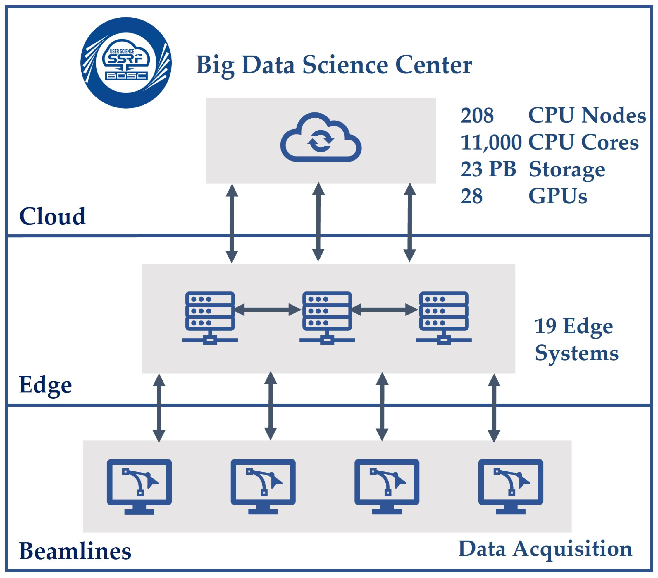
Figure 1. Hardware architecture of the CEHIS at the SSRF.
Applsci 13 05387 g001
Figure 2. Data processing workflow of the SSRF MX beamline.
Applsci 13 05387 g002
Figure 3. A computational job and tasks, including the task instances that compose it.
Applsci 13 05387 g003
Figure 4. Service delivery paradigm of the CEHIS.
Applsci 13 05387 g004
Figure 5. Reinforcement learning.
Applsci 13 05387 g005
Figure 6. Implementation of the task scheduling with a policy gradient-based DRL algorithm in the CEHIS.
Applsci 13 05387 g006
Figure 7. Policy network.
Applsci 13 05387 g007
Figure 8. Makespan of the CHEIS and CC systems using different task scheduling algorithms.
Applsci 13 05387 g008
Figure 9. (a) Simulation time of the CEHIS and CC systems using different task scheduling algorithms; (b) average completion time of the CEHIS and CC systems using different task scheduling algorithms.
Applsci 13 05387 g009
Figure 10. Average slowdown of the CEHIS and CC systems using different task scheduling algorithms.
Applsci 13 05387 g010
Table 1. HPC Cluster Computing System I at the SSRF.
NodesNumberConfiguration
CPU Node48Intel Xeon Gold 6104
(2.3 GHz, 18 Core) × 2
16 GB DDR4 Memory × 8
Fat Node1Intel Xeon E7-8860v4
(2.2 GHz, 18 Core) × 16
16 GB DDR4 Memory × 128
PCle GPU Node4Intel Xeon 5118 (2.3 GHz, 12 Core) × 2
NVIDIA Tesla P100 GPU Card × 2
16 GB DDR4 Memory × 8
NVLINK GPU Node1Intel Xeon Gold 6132
(2.6 GHz, 14 Core) × 4
NVIDIA Tesla P100 GPU Card × 4
32 GB DDR4 Memory × 32
Table 2. HPC Cluster Computing System Ⅱ at the SSRF.
NodesNumberConfiguration
CPU Node160Intel Xeon Gold 5320
(2.2 GHz, 26 Core) × 2
32 GB DDR4 Memory × 8
Fat Node2Intel Xeon 8260
(2.4 GHz, 24 Core) × 8
16 GB DDR4 Memory × 64
GPU Node4Intel Xeon 6226R
(2.3 GHz, 18 Core) × 2
NVIDIA A100 GPU Card × 4
16 GB DDR4 Memory × 12
Table 3. Edge computing system at the SSRF.
CPUMemoryStorageGPUApplicationBeamline
x86 × 2
2.0 GHz
64 cores
512 GB184.32 TB
Intel S4510
SSD × 24
Big metadata
Real-time pipelines
BL02U1
BL10U2
x86 × 2
2.9 GHz
16 cores
192 GB184.32 TB
Intel S4510
SSD × 24
RTX5000 × 23D data pipelinesBL12SW
BL13U
x86 × 2
2.9 GHz
16 cores
192 GB192 TB
7200 RPM × 12
Big metadataBL16U2
x86 × 2
2.0 GHz
64 cores
512 GB96 TB
7200 RPM × 6
Big metadataBL03SB
BL13SSW
x86 × 2
2.9 GHz
16 cores
192 GB48 TB
7200 RPM × 3
RTX3080TI3D data pipelines
Big metadata
Real-time pipelines
BL17M
BL18B
x86 × 2
2.9 GHz
16 cores
192 GB184.32 TB
Intel S4510
SSD × 24
RTX5000 × 23D data pipelinesBL12SW
BL13U
etc.
Table 4. Performance evaluation based on 30 jobs scheduled with the DRL.
RAFFTetrisDRL
Makespan666673666632
ST1.672.073.7786.13
ACT39.4238.0138.7538.82
AS1.211.191.171.17
Table 5. Performance evaluation based on 50 jobs scheduled with the DRL.
RAFFTetrisDRL
Makespan1316133114331251.41
ST6.266.3618.56223.19
ACT54.5242.9745.8248.84
AS2.031.591.321.32
Disclaimer/Publisher’s Note: The statements, opinions and data contained in all publications are solely those of the individual author(s) and contributor(s) and not of MDPI and/or the editor(s). MDPI and/or the editor(s) disclaim responsibility for any injury to people or property resulting from any ideas, methods, instructions or products referred to in the content.