
Multi-Output Based Hybrid Integrated Models for Student Performance Prediction


Abstract
:1. Introduction
2. Related Work
3. Materials and Methods
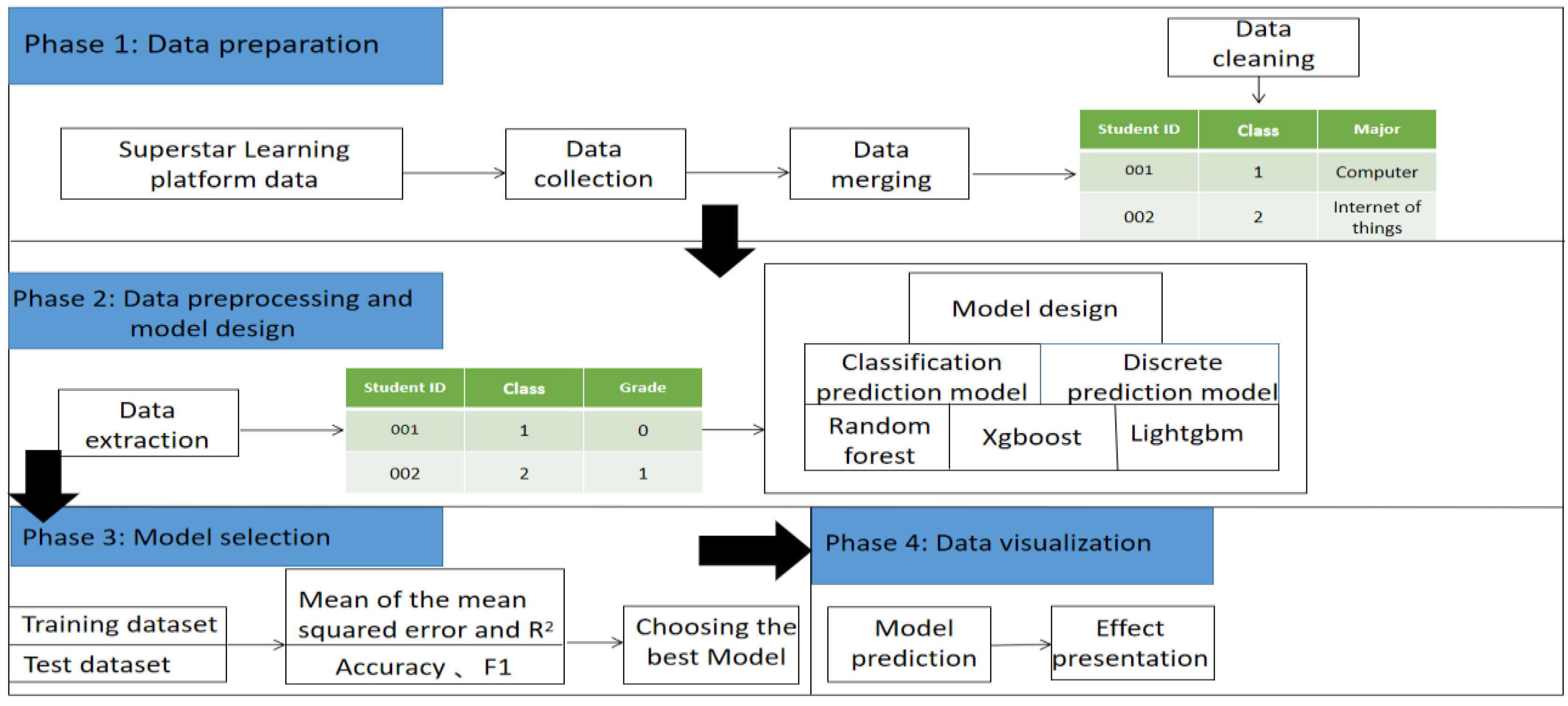
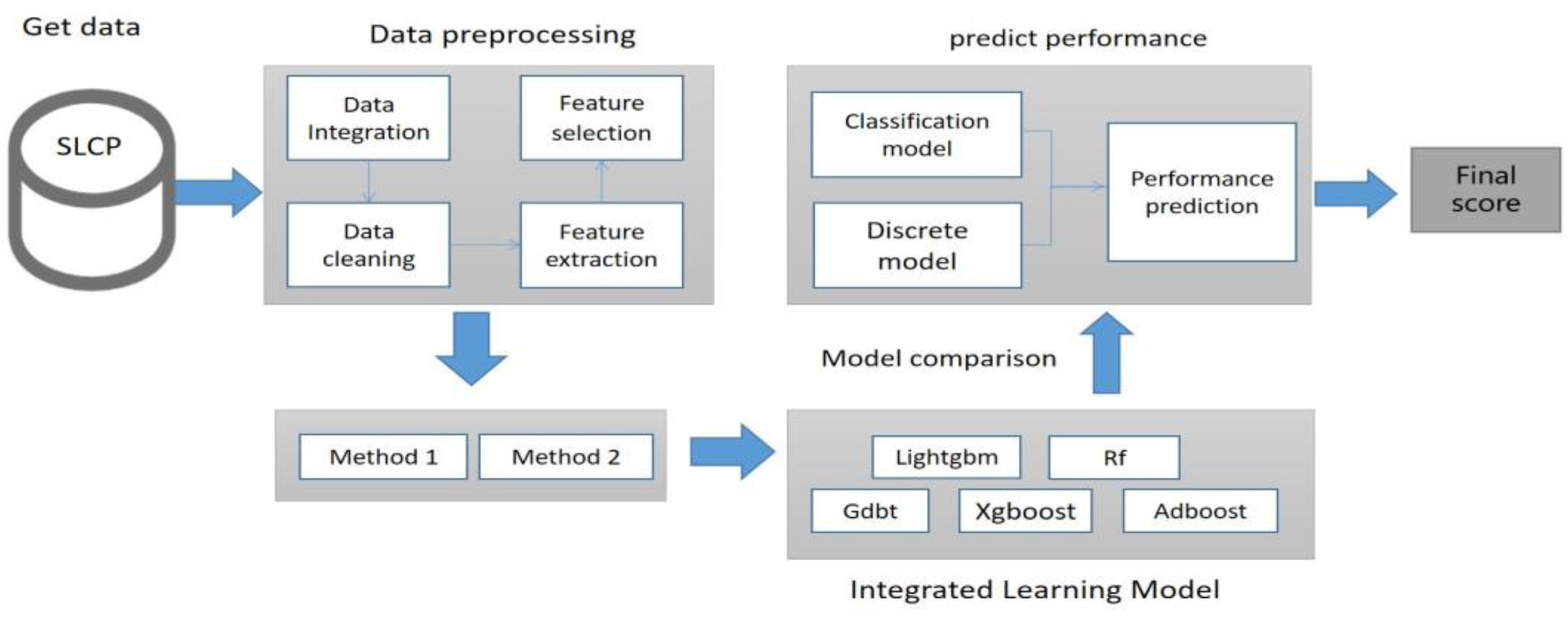
3.1. Multi-Output Prediction Model Framework
3.2. Data Set
3.3. Data Preprocessing
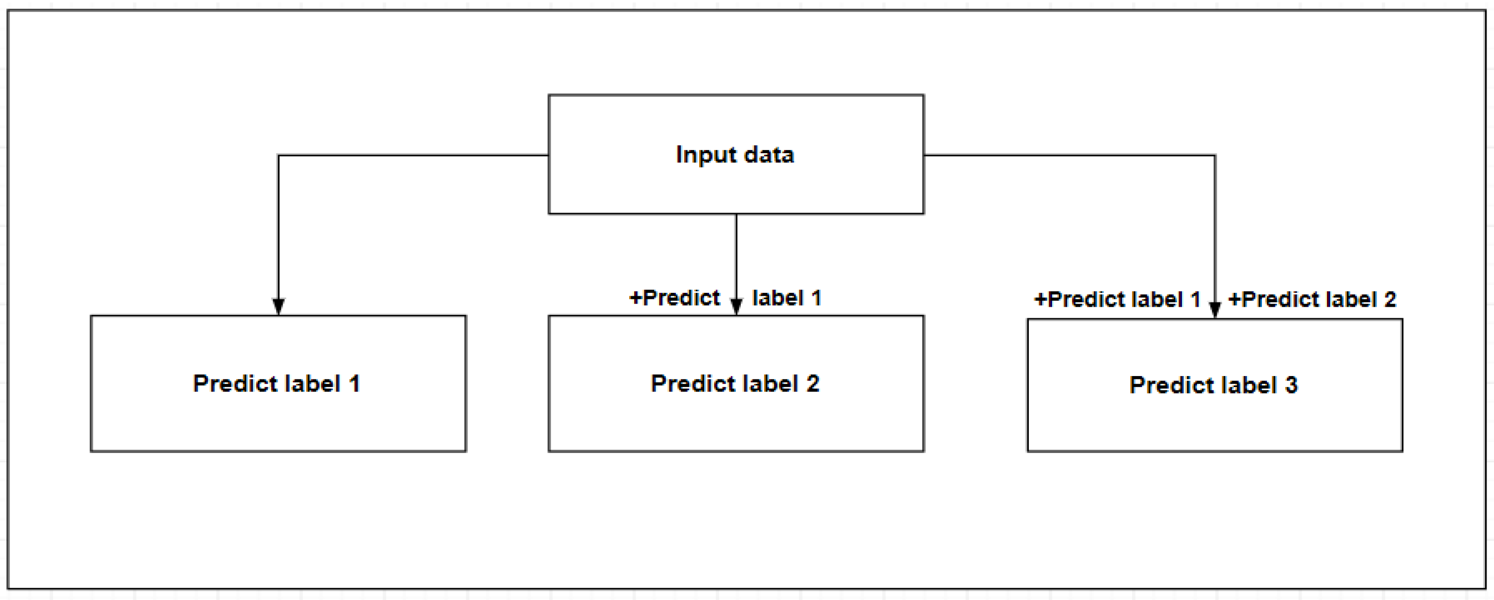
3.4. Model Design
| Algorithm 1: Multi-output model under different methods |
| Input: training data |
| Output: mid-term grade, homework grade, experiment grade, final grade |
| 1 Start |
| 2 Import necessary packages and read data |
| 3 Perform data preprocessing |
| 3.1 Feature attribute extraction |
| 3.2 Missing value padding |
| 3.3 Text data conversion |
| 4 Use classifier/regression to predict |
| 4.1 Use method 1 to predict different models |
| 4.2 Use method 2 to predict different models |
| 4.2 Select model parameters according to the evaluation index using tenfold cross validation |
| 5 Compare the effects of different models according to evaluation indicators |
| 6 Combine the most appropriate model for prediction |
| 7 End |
3.5. Model Evaluation
3.6. Model Parameter Configuration
3.7. Model Comparison
3.7.1. Comparison of Classification Models
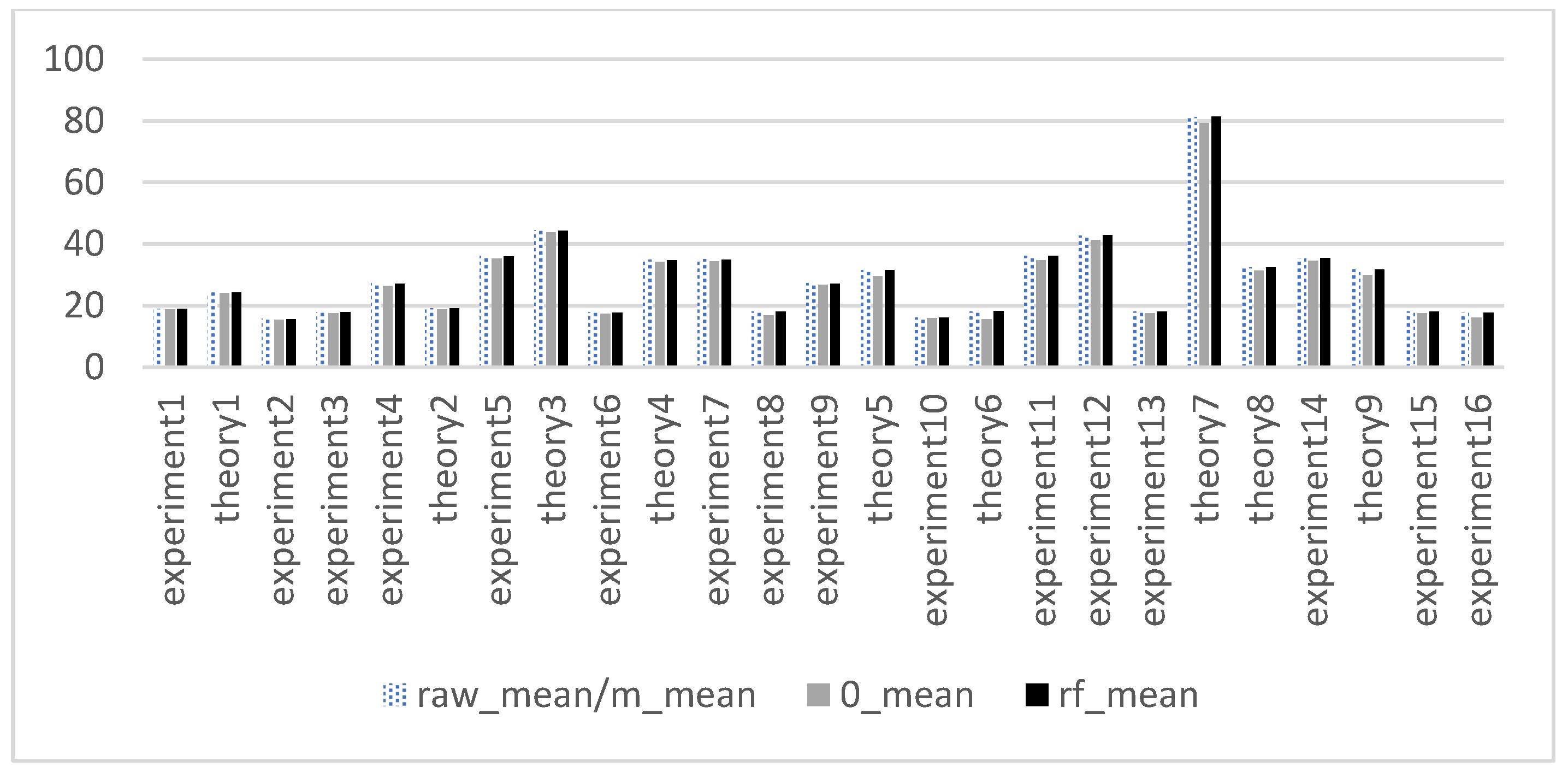
3.7.2. Comparison of Discrete Models
3.8. Model Determination
4. Experimental Setup
5. Experimental Results and Discussion
6. Conclusions
Author Contributions
Funding
Institutional Review Board Statement
Informed Consent Statement
Data Availability Statement
Conflicts of Interest
References
- Xiao, R.; Qu, J.; Wang, H.; Wang, M. Research on Clustering, Causes and Countermeasures of College Students’ Online Learning Behavior. Softw. Guide. 2022, 6, 230–235. [Google Scholar]
- Yağcı, M. Educational data mining: Prediction of students’ academic performance using machine learning algorithms. Smart Learn. Environ. 2022, 9, 1–19. [Google Scholar] [CrossRef]
- Xu, H. Prediction of Students’ Performance Based on the Hybrid IDA-SVR Model. Complexity 2022, 2022, 1845571. [Google Scholar] [CrossRef]
- Roslan, M.H.B.; Chen, C.J. Predicting students’ performance in English and Mathematics using data mining techniques. Educ. Inf. Technol. 2022, 28, 1427–1453. [Google Scholar] [CrossRef] [PubMed]
- Li, X.; Zhang, Y.; Cheng, H. Student achievement prediction using deep neural network from multi-source campus data. Complex Intell. Syst. 2022, 8, 5143–5156. [Google Scholar] [CrossRef]
- Luo, Y.; Han, X. Exploring the interpretability of the mixed curriculum student achievement prediction model. China Distance Education. 2022, 6, 46–55. [Google Scholar]
- Kukkar, A.; Mohana, R.; Sharma, A.; Nayyar, A. Prediction of student academic performance based on their emotional wellbeing and interaction on various e-learning platforms. Educ. Inf. Technol. 2023, 1–30. [Google Scholar] [CrossRef]
- Ban, W.; Jiang, Q.; Zhao, W. Research on accurate prediction of online learning performance based on multi algorithm fusion. Modern Distance Education. 2022, 3, 37–45. [Google Scholar]
- Ortiz-Vilchis, P.; Ramirez-Arellano, A. Learning Pathways and Students Performance: A Dynamic Complex System. Entropy 2023, 25, 291. [Google Scholar] [CrossRef] [PubMed]
- Ma, Y.; Cui, C.; Yu, J. Multi-task MIML learning for pre-course student performance prediction. Front. Comput. Sci. 2020, 14, 1–10. [Google Scholar] [CrossRef]
- Shen, G.; Yang, S.; Huang, Z.; Yu, Y.; Li, X. The prediction of programming performance using student profiles. Educ. Inf. Technol. 2022, 28, 725–740. [Google Scholar] [CrossRef]
- Yekun, E.A.; Haile, A.T. Student performance prediction with optimum multilabel ensemble model. J. Intell. Syst. 2021, 30, 511–523. [Google Scholar] [CrossRef]
- Kumar, A. Introduction and Practice of Integrated Learning: Principles, Algorithms and Applications. Beijing:Chem. Ind. Press. 2022, 2, 9–11. [Google Scholar]
- Wang, H.; Wang, G. Improving random forest algorithm by Lasso method. J. Stat. Comput. Simul. 2021, 91, 353–367. [Google Scholar] [CrossRef]
- Ma, M.; Zhao, G.; He, B. XGBoost-based method for flash flood risk assessment. J. Hydrol. 2021, 598, 126382. [Google Scholar] [CrossRef]
- Wang, Y.; Wang, T. Application of improved LightGBM model in blood glucose prediction. Appl. Sci. 2020, 10, 3227. [Google Scholar] [CrossRef]
- Heo, J.; Yang, J.Y. AdaBoost based bankruptcy forecasting of Korean construction companies. Appl. Soft Comput. 2014, 24, 494–499. [Google Scholar] [CrossRef]
- Zhang, C.; Zhang, Y.; Shi, X. On incremental learning for gradient boosting decision trees. Neural Process. Lett. 2019, 50, 957–987. [Google Scholar] [CrossRef]
- Zhou, Z. Machine Learning; Tsinghua University Press: Beijing, China, 2016; pp. 28–32. [Google Scholar]


| Serial Number | Characteristic Name | Data Type | Characteristic Meaning |
|---|---|---|---|
| 1 | name | varchar | name |
| 2 | student ID | varchar | student number |
| 3 | class | varchar | class |
| 4 | major | varchar | major |
| 5 | faculty | varchar | department |
| Serial Number | Characteristic Name | Data Type | Characteristic Meaning | Time |
|---|---|---|---|---|
| 1 | task_click | int | number of tasks completed | |
| 2 | view_time | double | video viewing duration | |
| 3 | discuss_count | int | number of discussions | |
| 4 | study_count | int | learning times | |
| 5 | sign | int | sign-in times | |
| 6 | experiment1 | double | experiment result 1 | 1 March 2022 |
| 7 | theory1 | double | theoretical score 1 | 6 March 2022 |
| 8 | experiment2 | double | experiment result 2 | 11 March 2022 |
| 9 | experiment3 | double | experiment result 3 | 16 March 2022 |
| 10 | experiment4 | double | experiment result 4 | 21 March 2022 |
| 11 | theory2 | double | theoretical score 2 | 26 March 2022 |
| …… | …… | …… | …… | …… |
| 32 | end_score | double | final exam | 1 July 2022 |
| Major | Qualified in the Interim | Intermediate Unqualified | Qualified at the End of the Period | Unqualified at the End of the Period | Total |
|---|---|---|---|---|---|
| Computer Science and Technology | 29 | 15 | 16 | 28 | 44 |
| Software engineering | 30 | 9 | 29 | 10 | 39 |
| Intelligent science and technology | 20 | 17 | 9 | 28 | 37 |
| Other | 0 | 2 | 0 | 2 | 2 |
| Total | 79 | 43 | 54 | 68 | 122 |
| Percentage | 64.75% | 35.25% | 44.26% | 55.74% |
| True Value | ||||
|---|---|---|---|---|
| Estimate | p | n | Total | |
| P’ | True positive (TP) | False positive (FP) | P’ | |
| n’ | False negative (FN) | True negative (TN) | N’ | |
| Total | P | N | ||
| Model | Parameter Settings | Accuracy/MSE_a |
|---|---|---|
| m_xgboost(midterm exam) | learning_rate=0.1,max_depth=2, n_estimators=100,max_delta_step=0.2 | 0.7837 |
| 0_xgboost(midterm exam) | learning_rate=0.9,n_estimators=50, min_child_weight=2,max_depth=2 | 0.7567 |
| 0_gdbt(midterm exam) | random_state=40,learning_rate=0.55,n_estimators=100 | 0.7567 |
| m_xgboost(final exam) | max_depth=3,learning_rate=0.19,n_estimators=100, min_child_weight=1,max_delta_step=0.4 | 0.7837 |
| r_xgboost(final exam) | learning_rate=0.70,n_estimators=100, min_child_weight=1,max_delta_step=0.2 | 0.7567 |
| 0_xgboost(final exam) | learning_rate=0.90,max_depth=8, min_child_weight=1,max_delta_step=0.5 | 0.7297 |
| m_gdbt(process grade) | random_state=40,learning_rate=0.01,subsample=0.2 | 16.7699 |
| m_randomforests(process grade) | random_state=40,max_depth=2,min_samples_leaf=10 | 17.1784 |
| r_gdbt(process grade) | random_state=40,learning_rate=0.01,subsample=0.2 | 17.7929 |
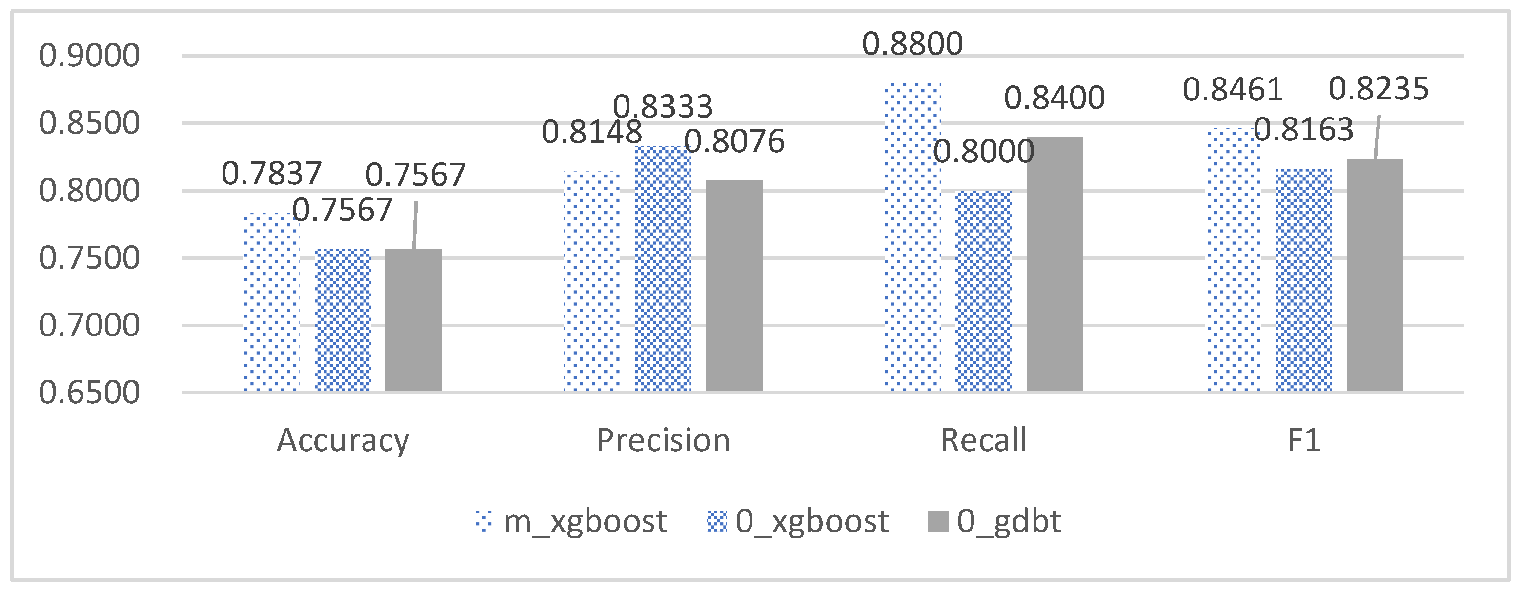
| Model | Accuracy | Precision | Recall | F1 |
|---|---|---|---|---|
| m_xgboost | 0.7837 | 0.8148 | 0.88 | 0.8461 |
| 0_xgboost | 0.7567 | 0.8333 | 0.8 | 0.8163 |
| 0_gdbt | 0.7567 | 0.8076 | 0.84 | 0.8235 |
| m_lgb | 0.7567 | 0.8333 | 0.8 | 0.8163 |
| m_gdbt | 0.7567 | 0.8076 | 0.84 | 0.8235 |
| r_lgb | 0.7567 | 0.8333 | 0.8 | 0.8163 |
| r_gdbt | 0.7567 | 0.8333 | 0.8 | 0.8163 |
| 0_lgb | 0.7297 | 0.8 | 0.8 | 0.8 |
| m_randomforests | 0.7297 | 0.7586 | 0.88 | 0.8148 |
| r_randomforests | 0.7297 | 0.7586 | 0.88 | 0.8148 |
| 0_randomforests | 0.7027 | 0.7333 | 0.88 | 0.8 |
| 0_adboost | 0.7027 | 0.7692 | 0.8 | 0.7843 |
| m_adboost | 0.7027 | 0.7692 | 0.8 | 0.7843 |
| r_xgboost | 0.7027 | 0.7916 | 0.76 | 0.7755 |
| r_adboost | 0.7027 | 0.75 | 0.84 | 0.7924 |
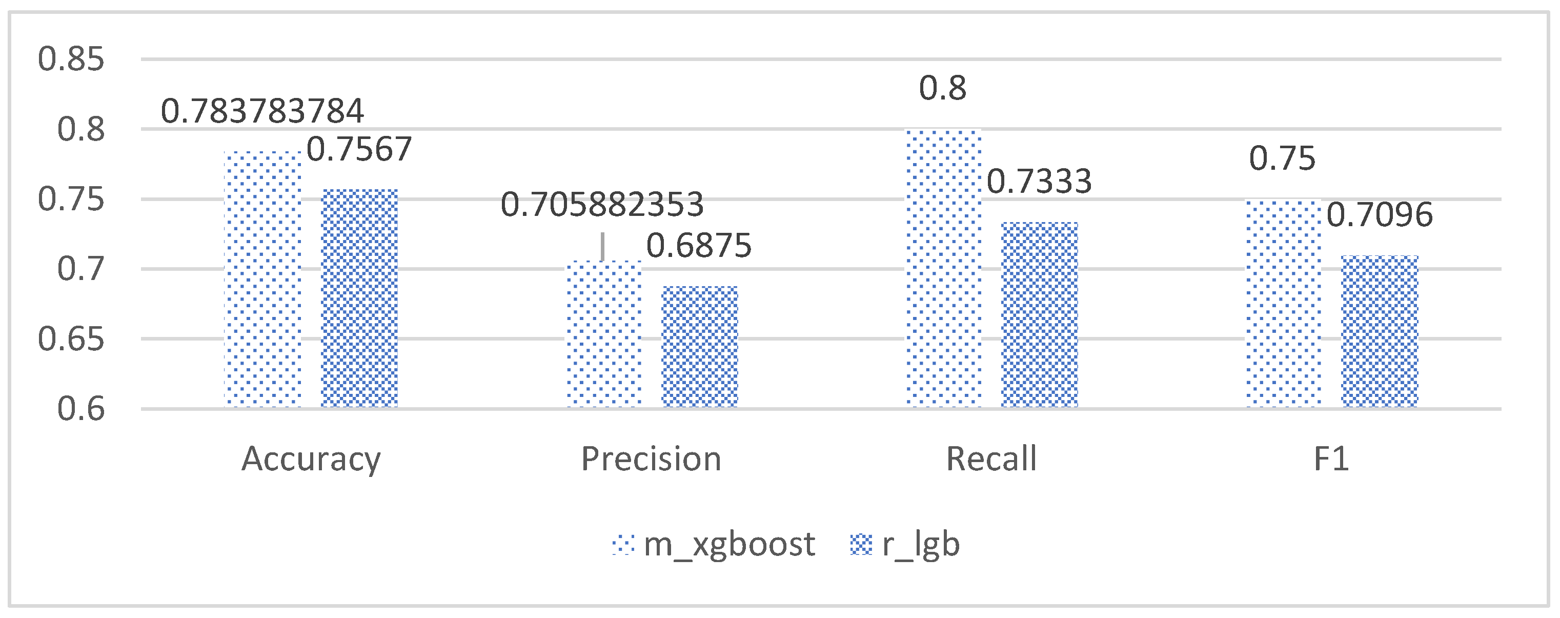
| Model | Accuracy | Precision | Recall | F1 |
|---|---|---|---|---|
| r_lgb | 0.7567 | 0.6875 | 0.7333 | 0.7096 |
| r_gdbt | 0.7567 | 0.7142 | 0.6666 | 0.6896 |
| r_adboost | 0.7567 | 0.7142 | 0.6666 | 0.6896 |
| m_xgboost | 0.7297 | 0.6470 | 0.7333 | 0.6875 |
| m_gdbt | 0.7297 | 0.6666 | 0.6666 | 0.6666 |
| r_xgboost | 0.7297 | 0.6923 | 0.6 | 0.6428 |
| 0_xgboost | 0.7027 | 0.6428 | 0.6 | 0.6206 |
| 0_gdbt | 0.7027 | 0.6666 | 0.5333 | 0.5925 |
| m_randomforests | 0.7027 | 0.6428 | 0.6 | 0.6206 |
| m_lgb | 0.7027 | 0.6111 | 0.7333 | 0.6666 |
| m_adboost | 0.7027 | 0.6428 | 0.6 | 0.6206 |
| 0_randomforests | 0.6756 | 0.6 | 0.6 | 0.6 |
| 0_lgb | 0.6756 | 0.6 | 0.6 | 0.6 |
| r_randomforests | 0.6756 | 0.6 | 0.6 | 0.6 |
| 0_adboost | 0.6486 | 0.5625 | 0.6 | 0.5806 |
| Model | Accuracy | Precision | Recall | F1 |
|---|---|---|---|---|
| m_xgboost | 0.7837 | 0.7058 | 0.8 | 0.75 |
| r_xgboost | 0.7567 | 0.7142 | 0.6666 | 0.6896 |
| 0_xgboost | 0.7297 | 0.6666 | 0.6666 | 0.6666 |
| 0_gdbt | 0.7297 | 0.6666 | 0.6666 | 0.6666 |
| m_gdbt | 0.7297 | 0.6666 | 0.6666 | 0.6666 |
| m_adboost | 0.7297 | 0.6666 | 0.6666 | 0.6666 |
| 0_lgb | 0.7027 | 0.6111 | 0.7333 | 0.6666 |
| 0_adboost | 0.7027 | 0.6 | 0.8 | 0.6857 |
| m_lgb | 0.7027 | 0.6111 | 0.7333 | 0.6666 |
| r_lgb | 0.7027 | 0.625 | 0.6666 | 0.6451 |
| r_gdbt | 0.7027 | 0.625 | 0.6666 | 0.6451 |
| r_adboost | 0.7027 | 0.625 | 0.6666 | 0.6451 |
| 0_randomforests | 0.6756 | 0.6 | 0.6 | 0.6 |
| m_randomforests | 0.6756 | 0.5882 | 0.6666 | 0.625 |
| r_randomforests | 0.6756 | 0.6 | 0.6 | 0.6 |
| Model | Process Performance Prediction (Method 1) | Process Performance Prediction (method 2) | ||||
|---|---|---|---|---|---|---|
| MSE_a | MAE_a | R2_a | MSE_a | MAE_a | R2_a | |
| m_gdbt | 17.737 | 2.8383 | 0.0167 | 16.769 | 2.7417 | 0.0375 |
| m_randomforests | 17.674 | 2.8063 | −0.001 | 17.178 | 2.8562 | 0.0052 |
| r_gdbt | 18.086 | 2.9610 | −0.005 | 17.792 | 2.8889 | 0.0050 |
| m_lgb | 18.132 | 2.8617 | 0.0058 | 18.037 | 2.8769 | 0.0057 |
| m_adboost | 18.944 | 2.9401 | −0.106 | 18.259 | 2.8527 | −0.073 |
| r_randomforests | 18.478 | 2.9623 | −0.011 | 18.489 | 2.9722 | −0.006 |
| r_lgb | 18.903 | 2.9905 | −0.004 | 18.794 | 2.9871 | −0.000 |
| r_adboost | 20.139 | 3.1394 | −0.124 | 19.707 | 2.9475 | −0.161 |
| m_xgboost | 24.787 | 3.3564 | −0.472 | 22.362 | 3.1556 | −0.348 |
| r_xgboost | 24.290 | 3.3235 | −0.393 | 23.006 | 3.3048 | −0.407 |
| 0_xgboost | 48.162 | 4.3520 | 0.4434 | 37.588 | 4.0346 | 0.4600 |
| 0_adboost | 47.694 | 3.6535 | 0.4937 | 43.786 | 3.5881 | 0.4735 |
| 0_gdbt | 48.850 | 4.3454 | 0.3914 | 47.318 | 4.1756 | 0.4171 |
| 0_randomforests | 56.879 | 4.3626 | 0.3538 | 49.833 | 4.0620 | 0.4664 |
| 0_lgb | 79.682 | 5.2129 | 0.1041 | 76.234 | 4.8797 | 0.1409 |
Disclaimer/Publisher’s Note: The statements, opinions and data contained in all publications are solely those of the individual author(s) and contributor(s) and not of MDPI and/or the editor(s). MDPI and/or the editor(s) disclaim responsibility for any injury to people or property resulting from any ideas, methods, instructions or products referred to in the content. |
© 2023 by the authors. Licensee MDPI, Basel, Switzerland. This article is an open access article distributed under the terms and conditions of the Creative Commons Attribution (CC BY) license (https://creativecommons.org/licenses/by/4.0/).
Share and Cite
Xue, H.; Niu, Y. Multi-Output Based Hybrid Integrated Models for Student Performance Prediction. Appl. Sci. 2023, 13, 5384. https://doi.org/10.3390/app13095384
Xue H, Niu Y. Multi-Output Based Hybrid Integrated Models for Student Performance Prediction. Applied Sciences. 2023; 13(9):5384. https://doi.org/10.3390/app13095384
Chicago/Turabian StyleXue, Han, and Yanmin Niu. 2023. "Multi-Output Based Hybrid Integrated Models for Student Performance Prediction" Applied Sciences 13, no. 9: 5384. https://doi.org/10.3390/app13095384
APA StyleXue, H., & Niu, Y. (2023). Multi-Output Based Hybrid Integrated Models for Student Performance Prediction. Applied Sciences, 13(9), 5384. https://doi.org/10.3390/app13095384