Integrated Path Tracking Controller of Underground Articulated Vehicle Based on Nonlinear Model Predictive Control

Abstract

This paper proposes an integrated path tracking controller for articulated vehicles. A nonlinear model-predictive control (NMPC)-based reference state tracker is designed as an upper-level controller to solve the vehicle’s longitudinal velocity and steering rate. A terminal cost is introduced into the NMPC to improve the controller’s stability. A lower-level controller is developed to translate upper-level solutions into vehicle actuators’ signals, including steering and driving controllers. The steering controller translates the steering rate into the linear velocity of the cylinder to calculate the required fluid volume and ultimately into the rotation speed of the steering motor. The neural network method is applied in the driving controller to ensure accuracy under different loadings. In order to investigate the effects of the path tracking controller, an articulated dump truck is adapted for the field tests by adding the steering-by-wire system and driving-by-wire system, respectively. Experimental verifications of the lower-level controller are performed. The results show that the controller can accurately satisfy the demand. Finally, the tracking performance of the integrated path tracking controller is analyzed experimentally under different reference velocities. The results indicate that tracking accuracy can be guaranteed.

1. Introduction

Articulated vehicles are widely used in underground mining environments since an articulated vehicle’s steering radius is smaller than a same-scale nonarticulated vehicle [1]. This maneuverability advantage is provided by the articulated vehicle’s steering approach: the vehicle’s hydraulic steering cylinders push or pull the front and rear body, making them rotate relative to each other and steer [2].

With the increasing demand for mineral resources, nearly 50 metal mines have been constructed at depths of more than 1000 m in China. Within the next ten to fifteen years, one-third of underground metal mines will enter 1000 m of mining depth [3]. Deep mining means more significant challenges, such as increased technical difficulty, harsh environments, and high safety risks [4]. As a result, the deep mining environment is unsuitable for long-term human operations. In this situation, developing autonomous mining technology is the inevitable option and necessary approach for deep resource extraction.

Autonomous driving is a precondition for autonomous mining. It mainly contains three major systems: sensing and perception, path planning, and path tracking [5]. Among them, path tracking control is a critical technology to realizing autonomous driving [6]. The path tracking control aims to ensure that the vehicle tracks the planned reference trajectory accurately, stably, and robustly [7]. In recent years, a large number of path tracking algorithms have been proposed, such as pure pursuit control, Stanley tracking algorithm, proportional–integral–derivative (PID) control, sliding mode control, adaptive control, $H_{\infty }$ control, linear quadratic regulator (LQR) control, and model-predictive control (MPC) [6,8,9]. MPC is increasingly used in current autonomous driving path tracking programs [10] because of its ability to handle multiple inputs and outputs and the advantage of considering system constraints [11,12,13]. Meanwhile, NMPC is increasingly used due to the improvement of the computational power of the controller and the update of the solution algorithm [14,15].

Compared to passenger vehicles, there are a few studies on MPC path tracking for articulated vehicles. Nayl presented a switching model-predictive control scheme for an articulated vehicle under varying slip angles [16,17,18]. Dou designed a dynamic error model-based MPC controller for steering control of an articulated vehicle [18]. Bai proposed NMPC path tracking controllers for articulated vehicles. By comparing with switching model-predictive control, NMPC can be used to improve the path tracking control accuracy [19]. Gao presented a novel model-based steering control for an articulated vehicle [20]. However, most of the papers mentioned above are based on simulation studies [16,17,18,19]. Only [20] contains an experimental investigation but solely includes steering control. More importantly, the parameters are fixed in these MPC controllers. However, due to the nature of the work of underground articulated mining vehicles, their loads change frequently. Therefore, a specific set of controller parameters does not allow the vehicle to maintain a good tracking accuracy throughout the entire work cycle.

Furthermore, the abovementioned path tracking controllers are insufficient to perform tracking experiments. Chassis controllers are needed to implement the control requirements of the path tracking controller; however, there are few descriptions of the chassis wire control system for underground articulated mining vehicles.

In addition, control-by-wire modifications are a prerequisite for realizing chassis control since most of the current articulated vehicles are designed to be driven manually. It is supposed to include steering-by-wire, driving-by-wire (acceleration, braking), and other actuators-by-wire systems (e.g., shoveling system, dump unloading system). For the steering-by-wire system, Rowduru proposes four kinds of solutions [2], including:

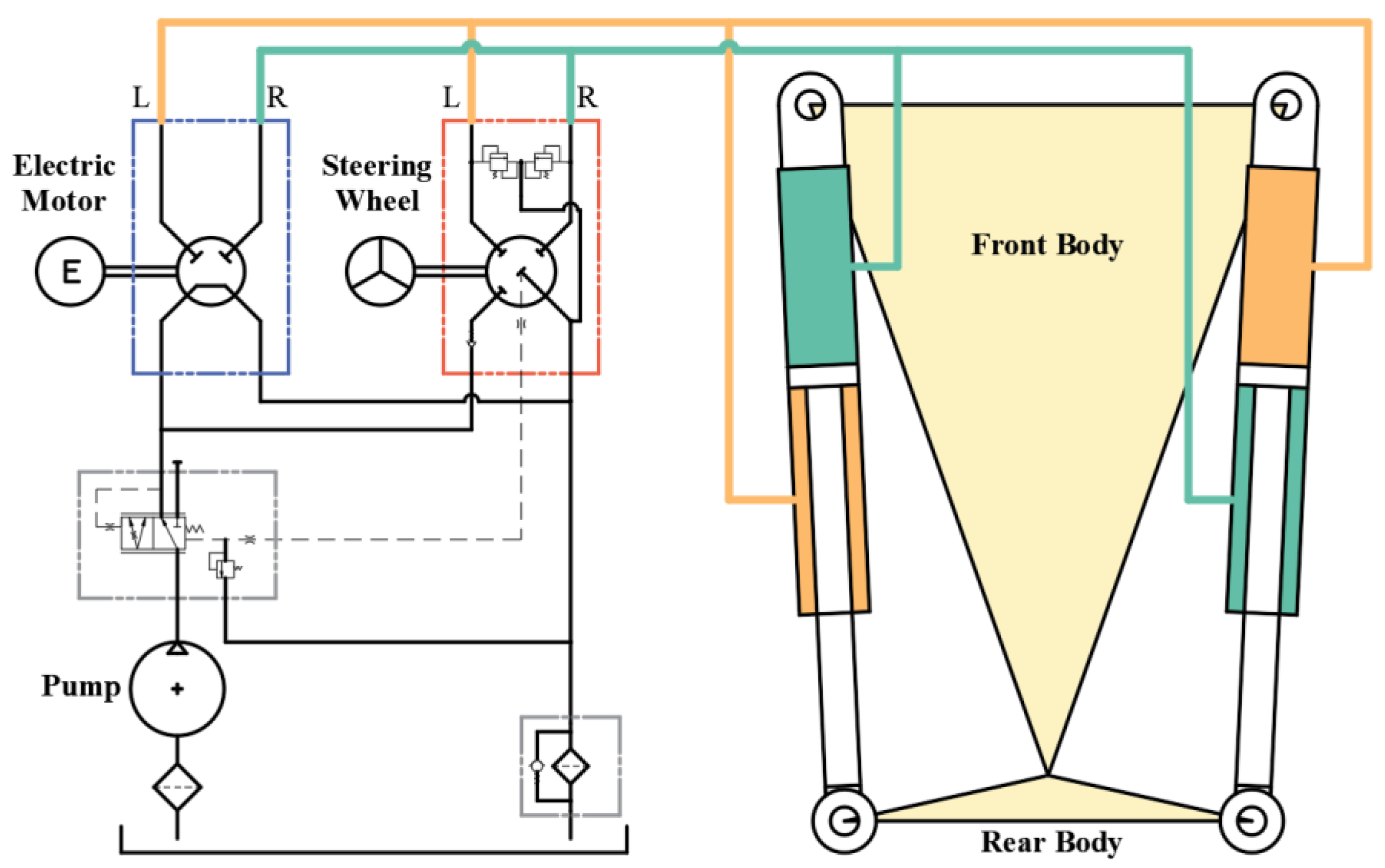
• A stepper motor provides torque to drive a hydraulic steering valve and control the articulated angle or angular speed [21];
• A proportional directional control valve (DCV) controls flow into the steering cylinder so that controls the articulated angular speed [22]. However, the proportional DCV usually has a dead zone [20], resulting in small articulated angular speeds not being achieved. Furthermore, when the oil pump is powered by the engine, the engine speed and the opening of the valve port will jointly affect the articulated angular speed, increasing the control difficulty;
• A motor controls the variable displacement pump (VDP) to manage the flow into the steering cylinder, so that controls the articulated angular speed. Compared to the DCV-controlled system, the response time of the pump-controlled actuation system is slower [23];
• Based on solution 3, a variable frequency drive (VFD) is applied to control the speed of an electric motor. Therefore, the flow entering into cylinders can be directly controlled either by the pump’s displacement or by the motor’s variable speed [24].

For the driving-by-wire system, there are different driving methods for different articulated vehicles, for instance, engine drive, motor drive, and hybrid drive. Different drive methods have different driving control methods. Therefore, the discussion will not be expanded here.

This paper presents an integrated path tracking controller for underground articulated mining vehicles. The controller includes an upper-level controller and a lower-level controller. The upper-level controller is an NMPC state tracker responsible for reducing errors between the vehicle and the reference path. The lower-level controller is a chassis controller accountable for meeting the control demands from the upper-level control. The lower-level controller includes a steering controller and a driving controller. A step motor is used to control the steering rate for the steering controller. It enables minor steering speeds, unlike other steering control methods with dead zones. A neural network control method is introduced for the driving controller to solve the complex driving relationships in articulated vehicles and to ensure the vehicle can cope with different load conditions. To implement the controller, a proposed solution is developed for the wire control modification of the articulated vehicle’s steering and driving systems. Based on this, this paper conducts an experimental study on the integrated path tracking controller. It verifies the controller’s accuracy, stability, and time performance during the experiment.

This paper is organized as follows. Section 2 elaborates on the design of an NMPC state tracker controller with terminal cost. Section 3 describes the design of a lower-level controller. Section 4 presents an overview of the articulated vehicle used for the experiments and the wire control adaptions. Section 5 presents the lower-level experimental verification and shows the integrated path tracking controller’s experimental results at different reference velocities. Finally, Section 6 concludes this paper.

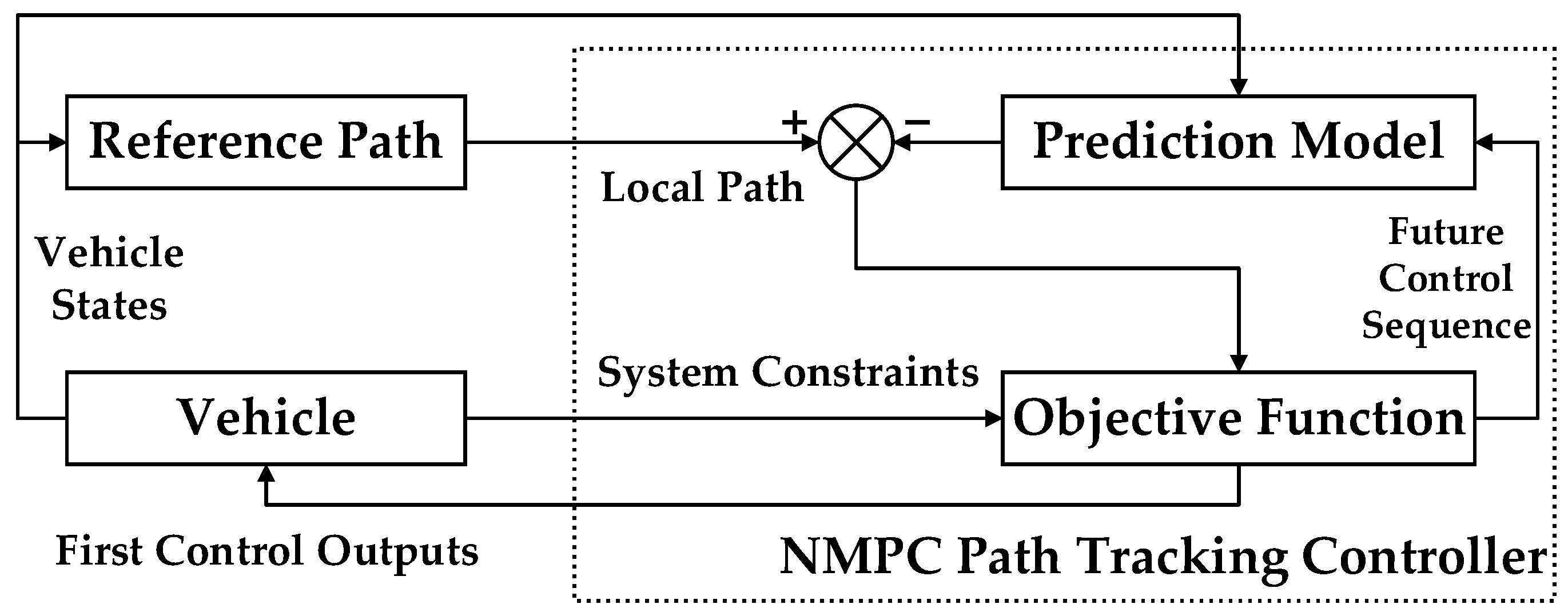
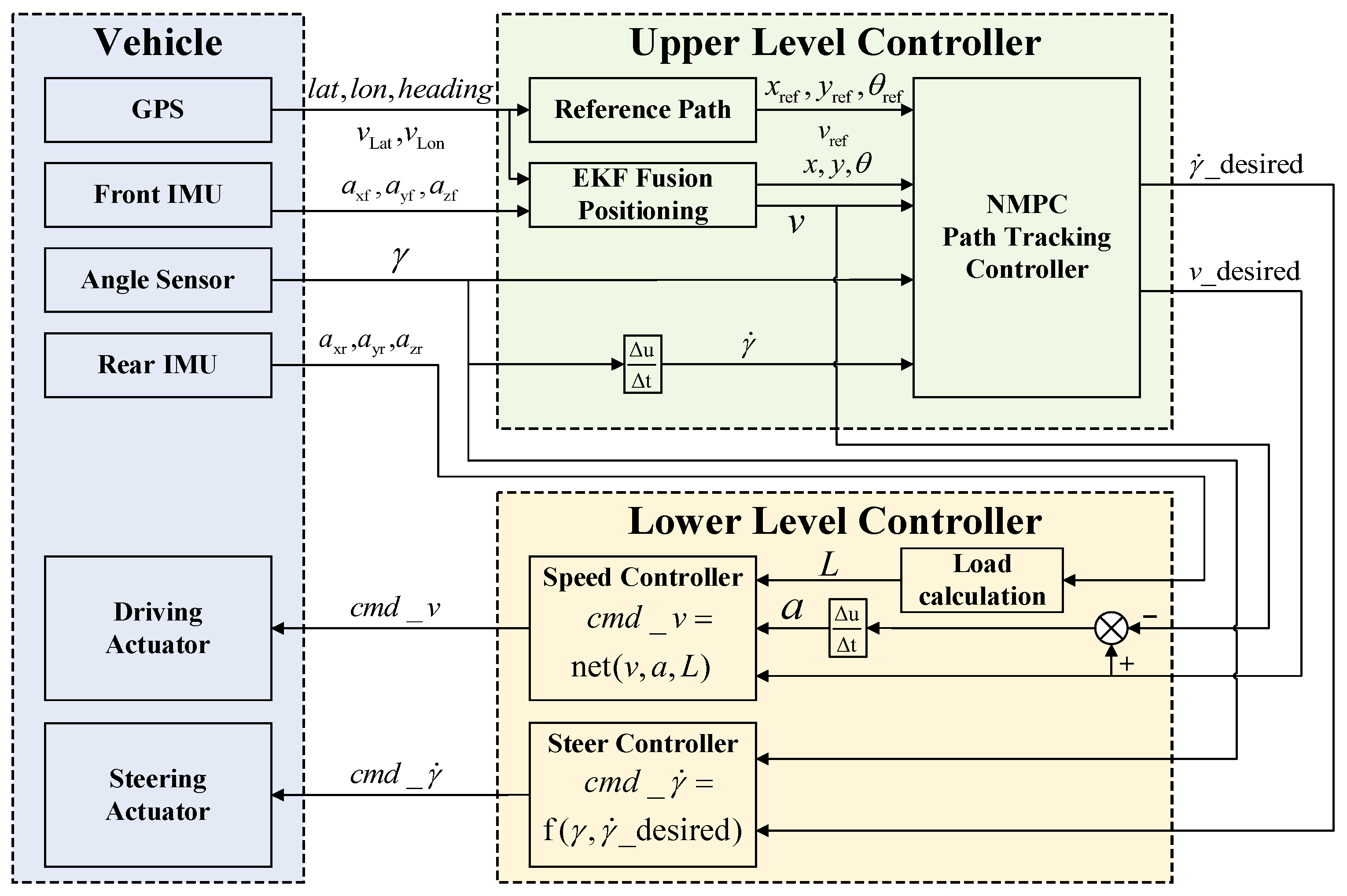
2. Upper-Level Controller

In this section, the NMPC controller design is discussed, and the mathematical formulation of the articulated vehicle model used in this work is explained.

2.1. Nonlinear Model-Predictive Control

NMPC can handle constraints explicitly, which comes from its model-based prediction of the future dynamic behavior of the system, by adding constraints to future inputs, outputs, or state variables, which can be represented explicitly in a nonlinear programming problem solved online. The NMPC closed-loop procedure is shown in Figure 1. The NMPC controller obtains the vehicle states and positioning by fusing the vehicle’s sensor information. At the same time, a path planning module gives a reference path based on the same information. The controller predicts the future state and calculates the error against the reference path. The controller obtains a group of control outputs by solving optimally under the constraints. The first group of control outputs is employed in the vehicle. After that, new states are obtained, and the subsequent control is performed.

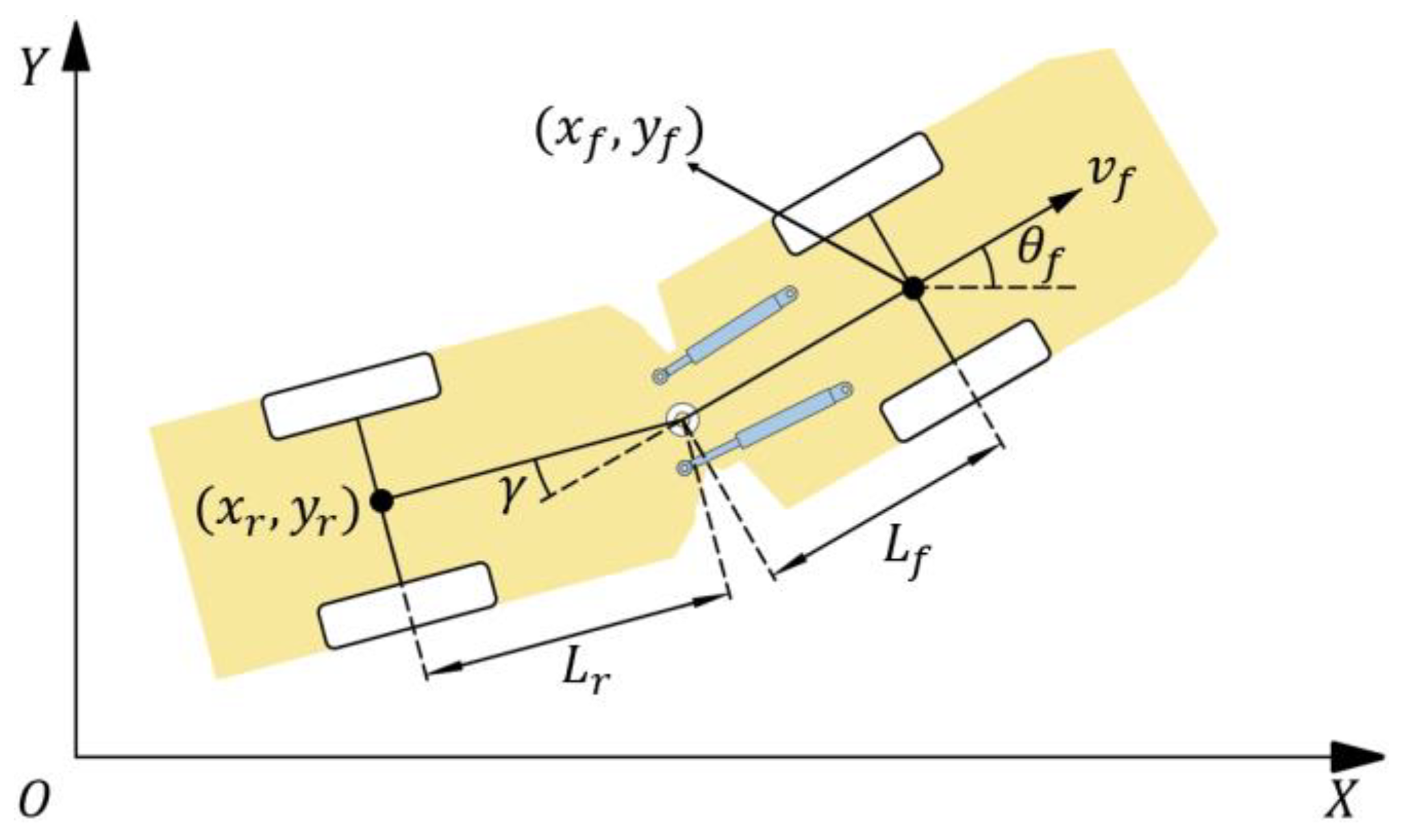
2.2. Predictive Model

A central part of model-predictive control is to have an accurate as well as computationally efficient system model. Therefore, the choice of using a kinematic model versus a dynamic model must take into account the desired balance between prediction accuracy and computational efficiency. When used as a prediction model, a kinematic model can calculate future states at a faster speed, which can improve the overall computation efficiency of the controller. However, when the vehicle speed is high, the prediction results may be inaccurate. On the other hand, a dynamic model used as a prediction model can produce more accurate prediction results. However, this would increase the computation time of the controller, and require additional input parameters, such as the vehicle’s acceleration and slip angle. These parameters are crucial in vehicle path tracking, but some of them cannot be directly measured by sensors, such as the slip angle. For example, Liu proposed a novel kinematic-model-based method for estimating vehicle slip angle (VSA) by combining information from GNSS and IMU to reduce the computation time and error of slip angle [25]. All these factors need to be considered when selecting a prediction model.

For underground mining operations, due to the width of the tunnel, road conditions, and safety reasons, vehicles are operated at low speeds, generally not more than 5 m/s. In this speed range, the kinematic model of the articulated vehicle can predict the future state with relative accuracy while ensuring real-time computational speed. Therefore, the nonlinear kinematic model of the articulated vehicle is used as the prediction model.

The kinematic model is depicted in the global coordinate $\mathrm{G}\left(X, Y\right),$ as shown in Figure 2. The front axle center is chosen as the vehicle state reference point. The derivation of the kinematic model of the articulated vehicle is given in the [19,26]. The vehicle’s nonlinear state-space system can be expressed as a matrix form:

$$\left[\begin{array}{c}\dot{x}\\ \dot{y}\\ \begin{array}{c}\dot{\theta }\\ \dot{\gamma }\end{array}\end{array}\right]=\left[\begin{array}{cc}\cos \theta & 0\\ \begin{array}{c}\sin \theta \\ \frac{\sin \gamma }{L_{\mathrm{f}}\cos \gamma +L_{\mathrm{r}}}\\ 0\end{array}& \begin{array}{c}0\\ \frac{L_{\mathrm{r}}}{L_{\mathrm{f}}\cos \gamma +L_{\mathrm{r}}}\\ 1\end{array}\end{array}\right]\left[\begin{array}{c}v\\ \mathsf{\omega }\end{array}\right]$$

(1)

where ${\left[\begin{array}{cccc}x& y& \theta & \gamma \end{array}\right]}^T$ represents the vehicle’s state, x and $y$ are the vehicle’s coordinate position, $\theta$ represents the heading angle, $\gamma$ is the articulated angle between the front and rear bodies, ${\left[\begin{array}{cc}v& \omega \end{array}\right]}^T$ represent vehicle’s control inputs, $v$ is the longitudinal speed, $\omega$ is the steering rate between two bodies, and $L_{\mathrm{f}}$ and $L_{\mathrm{r}}$ represent distances from the front and rear axle centers to the articulation point, respectively.

Assuming $\chi ={\left[\begin{array}{cccc}x& y& \theta & \gamma \end{array}\right]}^T$ and $u={\left[\begin{array}{cc}v& \omega \end{array}\right]}^T$, the system kinematics can be simply expressed as

$$\dot{\chi }=\mathrm{f}\left(\chi ,u\right)$$

(2)

In order to achieve the implementation of NMPC on a computer, the continuous nonlinear system is discretized using the Euler integrator:

$$\chi \left(k+1\right)=\chi \left(k\right)+T\mathrm{f}\left(\chi \left(k\right),\mathsf{\Delta }u\left(k\right)\right)$$

(3)

$$u\left(k\right)=u\left(k-1\right)+\mathsf{\Delta }u\left(k\right)$$

(4)

where T is the time step of the discretization. Δu(k) is control inputs’ increment. Its introduction ensures that it remains within constraints during the solving process.

2.3. Controller Design

The NMPC controller aims to ensure that the vehicle can accurately follow the desired trajectory. Hence, the error between the predicted states and the reference path is as tiny as possible. In addition, smooth control also needs to be guaranteed, which means that changes in the control inputs should be minimized. Consequently, the cost function of the NMPC controller can be expressed as

$$J\left(\chi \left(t\right),\mathsf{\Delta }{\mathcal{U}}_{\mathrm{t}}\right)={\displaystyle \sum }_{k=1}^{N_{\mathrm{p}}}\Vert \widehat{\chi }\left(t+k|t\right)-{\chi }_{\mathrm{ref}}{\left(t+k|t\right)\Vert }_{\mathrm{Q}}^2+{\displaystyle \sum }_{k=0}^{N_{\mathrm{c}}}\Vert \mathsf{\Delta }u{\left(t+k|t\right)\Vert }_{\mathrm{R}}^2$$

(5)

where $\widehat{\chi }\left(t+k|t\right)$ represents the predicted state of the vehicle based on the current measured state, ${\chi }_{\mathrm{ref}}\left(t+k|t\right)=$ ${\left[\begin{array}{cccc}{x}_{\mathrm{ref}}\left(t+k|t\right)& y_{\mathrm{ref}}\left(t+k|t\right)& {\theta }_{\mathrm{ref}}\left(t+k|t\right)& 0\end{array}\right]}^T$ is the status information of the reference path, $N_p$ is the predictive time domain, and $N_c$ is the control time domain. $Q$ is the weight matrix for tracking error, $R$ is the weight matrix for control inputs’ increment, and both are the positive define matrices.

In order to achieve higher tracking accuracy and improve the stability of the closed-loop system [27], a terminal cost is proposed based on the above NMPC controller as follows:

$$\mathcal{Z}\left(\chi \left(t\right)\right)=\Vert \widehat{\chi }\left(t+N_{\mathrm{p}}|t\right)-{\chi }_{\mathrm{ref}}{\left(t+N_{\mathrm{p}}|t\right)\Vert }_{\mathrm{P}}^2$$

(6)

where $P$ is the weight matrix for terminal cost.

In summary, the path tracking problem can be transformed into the MPC program presented in the following optimization problem:

$$\begin{array}{cc}\underset{\mathsf{\Delta }{\mathcal{U}}^{*}\left(t\right)}{\min }J\left(\chi \left(t\right),\mathsf{\Delta }\mathcal{U}\left(t\right)\right)& \\ \hfill =& \Vert \widehat{\chi }\left(t+N_{\mathrm{p}}|t\right)-{\chi }_{\mathrm{ref}}{\left(t+N_{\mathrm{p}}|t\right)\Vert }_{\mathrm{P}}^2+{\displaystyle {\displaystyle \sum }_{k=1}^{N_{\mathrm{p}}}}\Vert \widehat{\chi }\left(t+k|t\right)-{\chi }_{\mathrm{ref}}{\left(t+k|t\right)\Vert }_{\mathrm{Q}}^2\hfill \\ \hfill +& {\displaystyle {\displaystyle \sum }_{k=0}^{N_{\mathrm{c}}}}\Vert \mathsf{\Delta }u{\left(t+k|t\right)\Vert }_{\mathrm{R}}^2\hfill \end{array}$$

(7)

s.t.

$$\widehat{\chi }\left(0|0\right)=\chi \left(0\right)$$

$$\widehat{\chi }\left(t+1|t\right)=\widehat{\chi }(t|t)+T\mathrm{f}(\widehat{\chi }(t|t),\mathsf{\Delta }u(t|t))$$

(8)

$$u\left(t|t\right)=u\left(t-1|t\right)+\mathsf{\Delta }u\left(t|t\right)$$

(9)

$${\gamma }_{\min }\le \gamma \left(t+k|t\right)\le {\gamma }_{\max }, k=1, 2, 3,\dots ,N_{\mathrm{p}}$$

(10)

$$v_{\min }\le v\left(t+k|t\right)\le v_{\max }, k=1, 2, 3,\dots ,N_{\mathrm{c}}$$

(11)

$${\omega }_{\min }\le v\left(t+k|t\right)\le {\omega }_{\max }, k=1, 2, 3,\dots ,N_{\mathrm{c}}$$

(12)

$$\mathsf{\Delta }{v}_{\min }\le \mathsf{\Delta }v\left(t+k|t\right)\le \mathsf{\Delta }{v}_{\max }, k=0, 1, 2, 3,\dots ,N_{\mathrm{c}}$$

(13)

$$\mathsf{\Delta }{\omega }_{\min }\le \mathsf{\Delta }\omega \left(t+k|t\right)\le \mathsf{\Delta }{\omega }_{\max }, k=0, 1, 2, 3,\dots ,N_{\mathrm{c}}$$

(14)

where ${\gamma }_{\min }$ and ${\gamma }_{\max }$ are the articulated angle physical limits, $v_{\min }$ and $v_{\max }$ are longitudinal velocity limits, ${\omega }_{\min }$ and ${\omega }_{\max }$ are the steering rate limits, $\mathsf{\Delta }{v}_{\min }$ and $\mathsf{\Delta }{v}_{\max }$ are longitudinal acceleration limits, and $\mathsf{\Delta }{\omega }_{\min }$ and $\mathsf{\Delta }{\omega }_{\max }$ are steering acceleration limits.

After the optimal solution, a sequence of control outputs can be obtained as follows:

$$\mathsf{\Delta }{\mathcal{U}}^{*}\left(\mathrm{t}\right)={\left[\mathsf{\Delta }{u}^{*}\left(t|t\right),\mathsf{\Delta }{u}^{*}\left(t+1|t\right),\cdots ,\mathsf{\Delta }{u}^{*}\left(t+N_{\mathrm{c}}|t\right)\right]}^{\mathrm{T}}$$

(15)

The first group of the solution is applied to the vehicle, which can be expressed as

$$u\left(t\right)=\mathsf{\Delta }{u}^{*}\left(t|t\right)+u\left(t-1\right)$$

(16)

After applying the control inputs, the vehicle feeds back the current states again to correct states in the controller. NMPC performs a new round of predictive control based on the new reference path and the new states of the vehicle.

3. Lower-Level Controller

The control inputs from the upper-level controller are vehicle speed and steering rate, which are not the same as the vehicle’s actuation signals (engine throttle opening, brake command, and steering motor controller’s frequency). Hence, a lower-level controller is needed to convert the control information into actuator control signals.

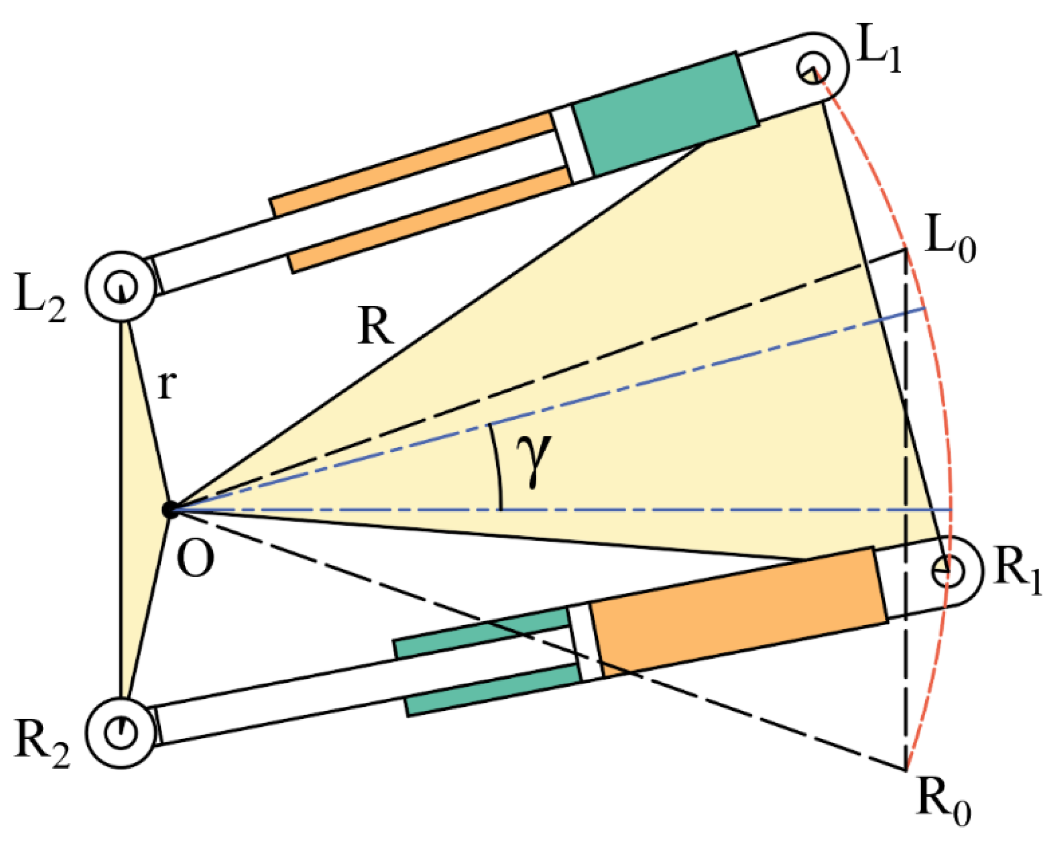
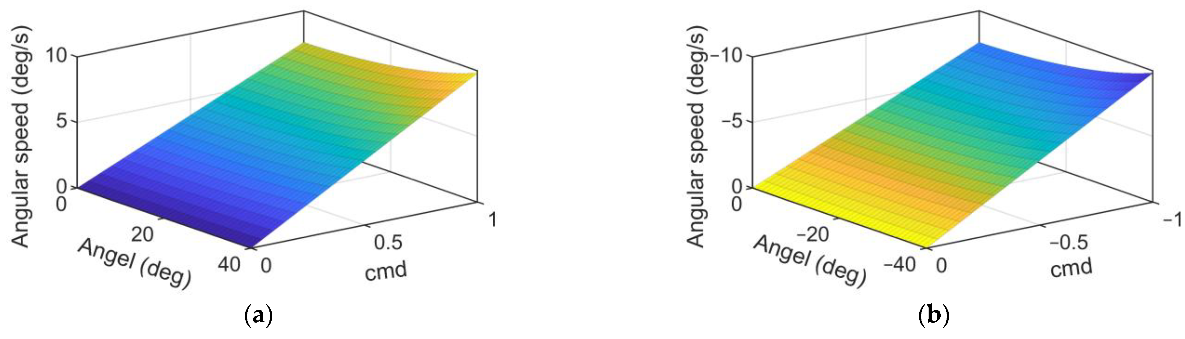
3.1. Steering Controller

Controller Design

Figure 3 shows a schematic diagram of the articulated steering structure’s movement. Since the steering hydraulic cylinders are fixed on the front and rear body, respectively, the articulated angular speed can be calculated from the linear speed of the piston push rod in the hydraulic steering cylinder. Based on this, the hydraulic fluid flow into the hydraulic cylinder can be controlled to determine the articulated angular speed, which is the steering speed of the vehicle.

The lengths of the hydraulic steering cylinder on the left and right sides are

$$\begin{array}{c}{L}_1{L}_2=\sqrt{r^2+R^2-2rR\cos ({\mathsf{\Omega }}_0+\gamma )}\\ R_1{R}_2=\sqrt{r^2+R^2-2rR\cos ({\mathsf{\Omega }}_0-\gamma )}\end{array}$$

(17)

where $R=O{R}_1$, $r=O{R}_2$, ${\mathsf{\Omega }}_0=\angle L_{0}O{L}_2=\angle R_{0}O{R}_2$.

The force arm corresponding to the pushing force of the hydraulic cylinder is

$$h_{\mathrm{L}1}=\frac{Rr\sin ({\mathsf{\Omega }}_0+\gamma )}{L_1{L}_2}, h_{\mathrm{L}2}=\frac{Rr\sin ({\mathsf{\Omega }}_0-\gamma )}{R_1{R}_2}$$

(18)

The expression for the relative linear velocity between the piston push rod in the cylinder and the piston cylinder is

$$\frac{\mathrm{d}{X}_L}{\mathrm{d}t}=h_{\mathrm{L}1}\dot{\gamma }, \frac{\mathrm{d}{X}_R}{\mathrm{d}t}=h_{\mathrm{L}2}\dot{\gamma }$$

(19)

where $X_{\mathrm{L}}$ and $X_{\mathrm{R}}$ are the corresponding displacements of the piston rods in the left and right hydraulic cylinders, respectively.

The flow rates in the hydraulic cylinders on the left and right sides are

$$Q_{\mathrm{L}}=A_{\mathrm{r}}\frac{\mathrm{d}{X}_{\mathrm{L}}}{\mathrm{d}t}, Q_{\mathrm{R}}=A_{\mathrm{P}}\frac{\mathrm{d}{X}_{\mathrm{R}}}{\mathrm{d}t}$$

(20)

where $A_{\mathrm{p}}$ and $A_{\mathrm{r}}$ are the practical cross-sectional areas of the rodless and rod chambers of the steering cylinder, respectively. As a result, the total flow provided by the steering valve should be

$$Q=Q_{\mathrm{L}}+Q_{\mathrm{R}}$$

(21)

From this, the frequency required for the steering motor controller can be calculated by

$$pulse=\frac{360\ast Q\ast s}{1.8\ast \eta \ast d}$$

(22)

where $s$ is the motor subdivision (20 in this paper), $\eta$ is the system efficiency (0.765, after experimental determination), and $d$ is the steering valve displacement ($500 \mathrm{mL}/\mathrm{r}$). We set $2000 \mathrm{Hz}$ as the maximum control command to obtain the normalized steering control command.

$$cmd=pulse/2000$$

(23)

Based on this, the angular speeds at different articulated angles and control commands are shown in Figure 4, with the left turn on the left figure and the right turn on the right figure.

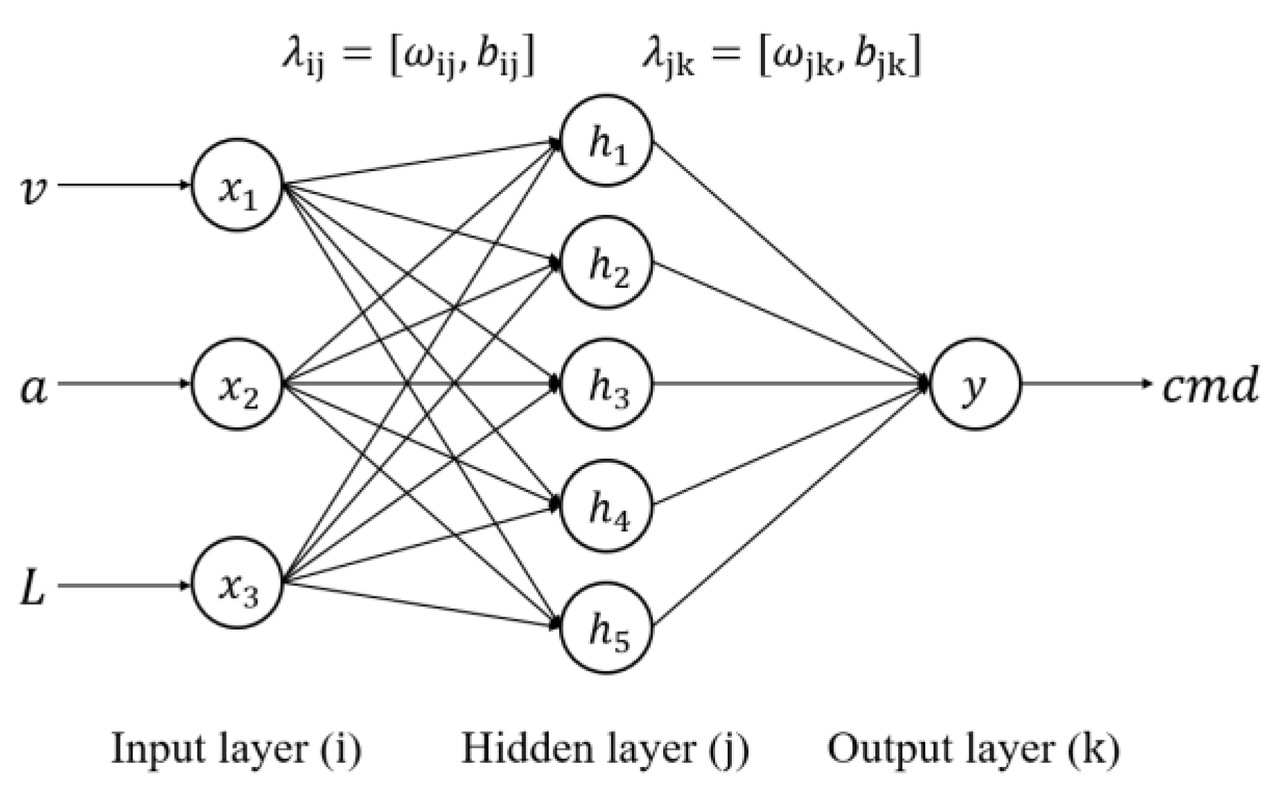
3.2. Driving Controller

3.2.1. Controller Design

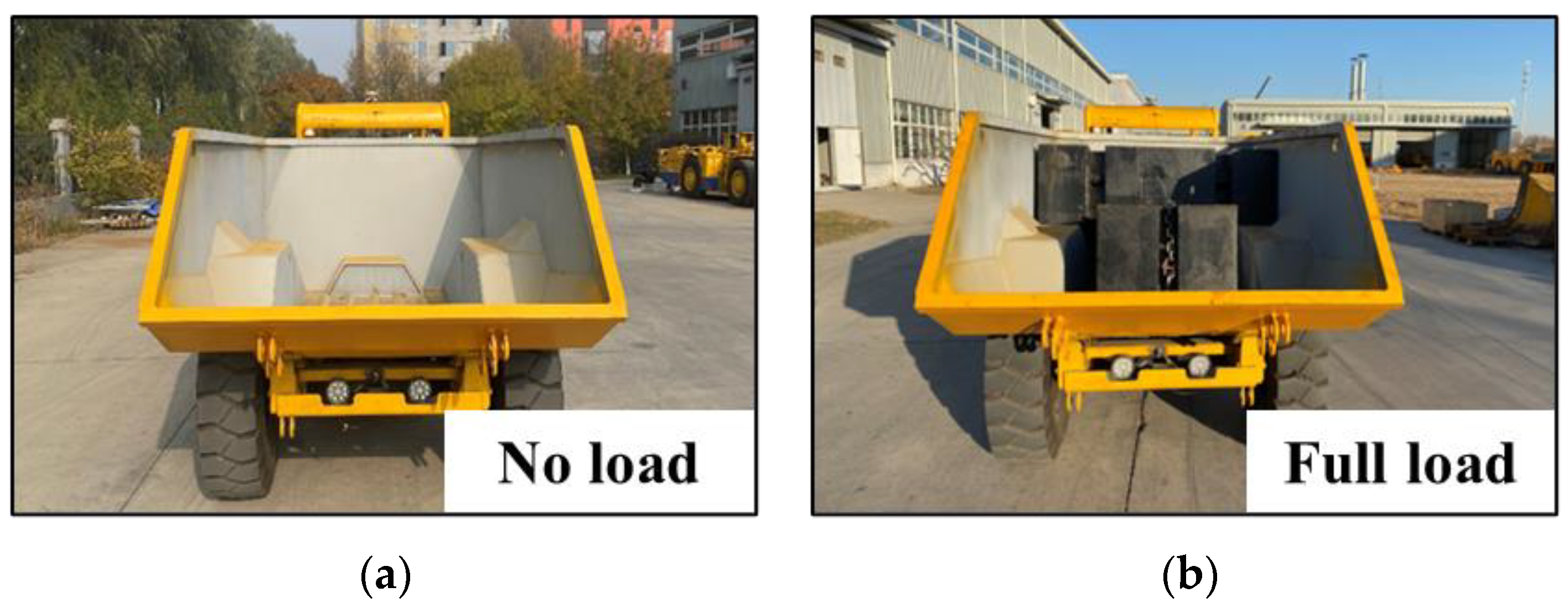
Underground mining articulated vehicles have a multivariable coupling relationship between engine throttle opening and vehicle speed due to the presence of torque converters and frequent load changes in the daily duty cycle. Conventional control algorithms, such as the look-up table or PID control, cannot effectively cover all situations. Therefore, this experimental vehicle chooses the backpropagation (BP) neural network approach as the solution for vehicle speed control. As shown in Figure 5, the BP neural network contains three layers: the input layer, the hidden layer, and the output layer. In the preliminary experiments, a fact is found that the vehicle’s speed control is mainly influenced by three factors: the present speed of the vehicle, the engine throttle opening, and the load.

Consequently, the input layer contains the current vehicle speed, desired acceleration, and load weight. The output layer is the control command (engine throttle opening). The current speed is obtained by Global Positioning System (GPS). The desired acceleration is calculated from the current and desired speeds obtained from NMPC, as shown in Equation (24).

$$a=\frac{v_{\mathrm{desired}}-v_{\mathrm{current}}}{T}$$

(24)

The load weight is calculated by the inertial measurement unit (IMU) data mounted on the vehicle’s rear body. The hidden layer uses five neurons, according to [28,29].

To obtain a sufficient neural network training dataset, the vehicle speed and acceleration are collected under different load cases with fixed and variable throttle input, as shown in Figure 6. The detailed conditions are as follows:

• Load: no-load ($0\mathrm{t}$), half-load ($3.5\mathrm{t}$), full-load ($7\mathrm{t}$).
• Throttle commands:

  a.

  Fixed: $10\%,20\%,30\%,40\%,50\%,60\%,70\%,80\%,90\%,100\%$;

  b.

  Varying (5 seconds step): $25\%\to 50\%\to 75\%\to 100\%$, $30\%\to 60\%\to 90\%$.

Data are collected five times for each condition. Thus, there are 180 sets of data.

3.2.2. Data Preprocessing

In the data preprocessing process, the rolling average filtering method is applied to remove the noise. The filter moves a window along the data and calculates the average of the data contained in each window. The following difference equation defines the moving average filter for vector $x$.

$${\overline{x}}_{\mathrm{i}}\left(n\right)=\frac{x_{\mathrm{i}}\left(n\right)+x_{\mathrm{i}}\left(n-1\right)+\dots +x_{\mathrm{i}}\left(n-\left(ws-1\right)\right)}{ws}$$

(25)

where $ws$ is the window size of the rolling window. In this paper, the window size is chosen to be $100$ because the velocity and acceleration data are acquired at a frequency of $100 \mathrm{Hz}$. Further, the data used for training is normalized to eliminate the effect of the difference in magnitude, as shown in Equation (26).

$${\overline{x}}_i{}^{\text{’}}\left(n\right)=\frac{{\overline{x}}_i\left(n\right)-{\overline{x}}_i{}_{\min }}{{\overline{x}}_i{}_{\max }-{\overline{x}}_i{}_{\min }}$$

(26)

where ${\overline{x}}^{’}\left(n\right)$ is the normalization result, ${\overline{x}}_{\max }$ is the maximum value in the sample, and ${\overline{x}}_{\min }$ is the minimum value in the sample.

3.2.3. Training

The activation function is chosen as a sigmoid function, as shown in Equation (27).

$$sigmoid\left(z\right)=\frac{1}{1+e^{-z}}$$

(27)

The mean square error (MSE) is chosen for the cost function in the training of the neural network, which can be expressed as

$$E=\frac{1}{M}{\displaystyle \sum }_{m=1}^M{(y\left(m\right)-\widehat{y}\left(m\right))}^2$$

(28)

where M is the size of the sample data, and $y_k$ and ${\widehat{y}}_k$ are the target value vector and the predicted value vector, respectively.

The stochastic gradient descent method is chosen for the training of the parameters.

The training process is shown in Algorithms 1 as follows.

Algorithms 1: The neural network training process.

Input: training set (control command: engine throttle opening) Input: training set (speed, acceleration) Input: parameters $\lambda$, the learning rate $\eta$, the number of iterations $S$

1: for $i=0$ to $S$ do

2: calculate $E$ for a small batch (number of samples $B” M$)

3: calculate $\frac{\partial E}{\partial \lambda }$ by back-propagation

4: $\mathsf{\Delta }\lambda \left(i+1\right)=\mathsf{\Delta }\lambda \left(i\right)-\eta \frac{\partial E}{\partial \lambda }$

5: $\lambda \left(i+1\right)=\lambda \left(i\right)+\mathsf{\Delta }\lambda \left(i+1\right)$ update the parameters

6: end for

7: Return $\lambda$; return the trained parameters

After training, the neural network can be represented as

$$Net:v,a,L\to cmd$$

(29)

where $Net$ refers to the neural network.

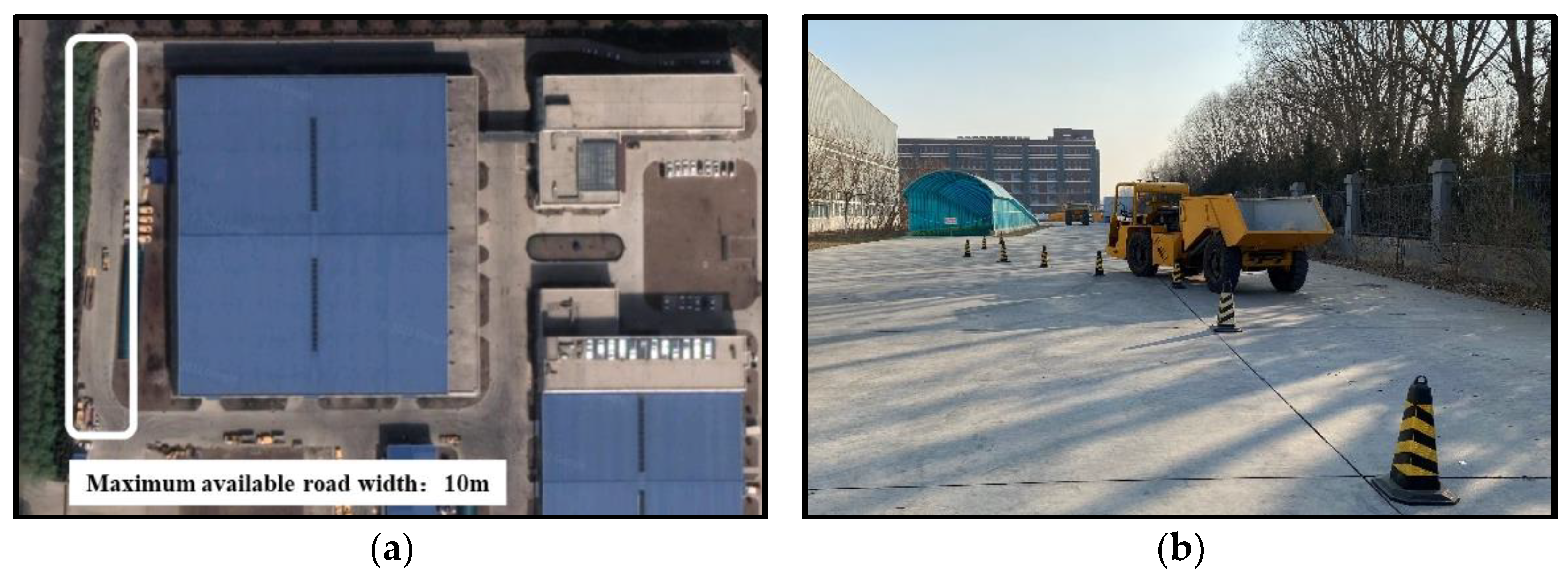
4. Experimental Vehicle

Three types of articulated vehicles are commonly used in underground metal mining: articulated rock drills for rock mining, load haul dump for shoveling, and articulated dump trucks for transporting rock in the tunnels.

In this article, the experimental vehicle is an AJK207 articulated dump truck manufactured by Beijing Anchises Technologies Co., Ltd. (Beijing, China). The vehicle configuration is shown in Figure 7. The vehicle’s cab, engine, and transmission are mounted on the front body and transmit drive to the front and rear axles. The cargo box is mounted on the rear body and has a maximum load capacity of seven tons. The vehicle is steered by two hydraulic cylinders mounted at the left and right of the articulated center, thus allowing the vehicle to have a small turning radius and increasing the passage efficiency in underground tunnels. The specific parameters of the vehicle are shown in

Table 1. Major parameters of the articulated dump truck.

Major Parameters	Unit	Value
Overall vehicle mass	Kg	7400
Maximum load capacity	Kg	7000
Maximum folding angle	deg	±42
Length from front axle to articulated center	mm	1620
Length from rear axle to articulated center	mm	1923
Inside steering radius	mm	3955
Outer steering radius	mm	5850
Tire rolling radius	mm	519
Wheelbase	mm	1322
Engine	DEUTZ-F6L914
Integrated torque converter transmission:	DANA-1201FT20000

.

This articulated dump truck is designed for manual driving. Therefore, the wire control function is equipped before achieving autonomous driving, including steering-by-wire system and driving-by-wire system.

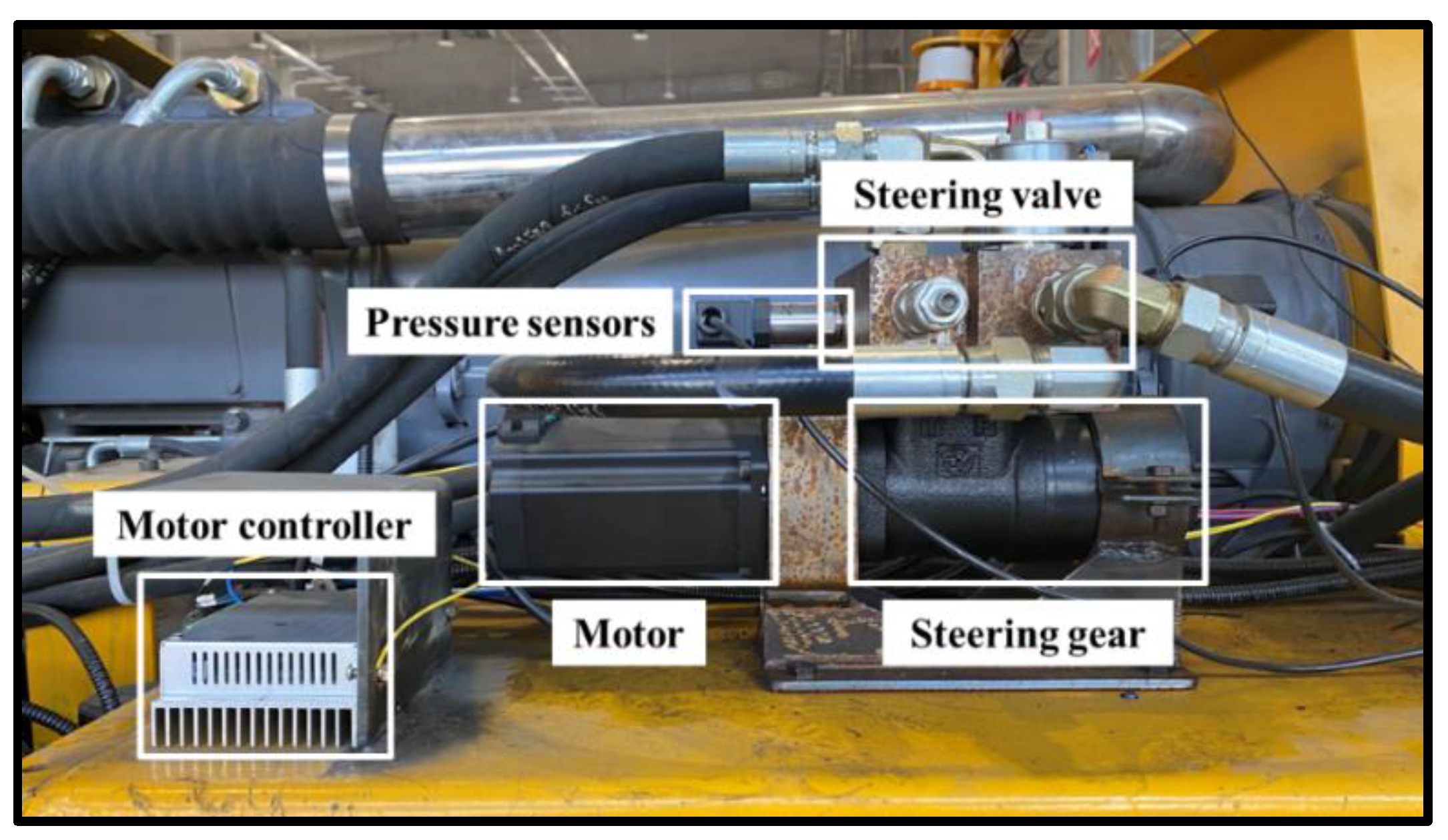
4.1. Steering-by-Wire System

As shown in Figure 8, the original steering method is to manually turn the steering wheel to drive the hydraulic steering valve mounted under the steering wheel (as shown in the orange box in Figure 8) to deliver hydraulic oil to the rod chamber of the left cylinder and the rodless chamber of the right cylinder to achieve left turn. The right turn supplies oil to the left cylinder’s rodless chamber and the right cylinder’s rod chamber. The vehicle’s oil pump is capable of pumping significantly more oil than the steering load, ensuring that the vehicle can be steered flexibly, which means that the vehicle can be steered by applying a small torque to the steering wheel. Based on this, the vehicle steering speed is determined only by the steering wheel rotation speed and current articulated angle.

In this paper, a stepper motor is used instead of human action. The stepper motor can control the angle and speed of its own rotation. The stepper motor is connected to a hydraulic steering valve identical to the original one (in the blue box in Figure 8). Similar to the steering wheel, when the motor rotates clockwise, the steering gear supplies oil to the left cylinder’s rod chamber and the right cylinder’s rodless chamber to achieve a left turn. In contrast, for a right turn, the motor rotates counterclockwise and supplies oil to the left cylinder’s rodless chamber and the right cylinder’s rod chamber.

The new steering valve is connected in parallel with the original one through a hydraulic valve block to ensure both the autonomous driving controller and the manual control. The actual vehicle installation of the newly equipped steering-by-wire system for is shown in Figure 9. The system includes a motor with a controller, a hydraulic steering valve, a parallel hydraulic valve block, and four pressure sensors.

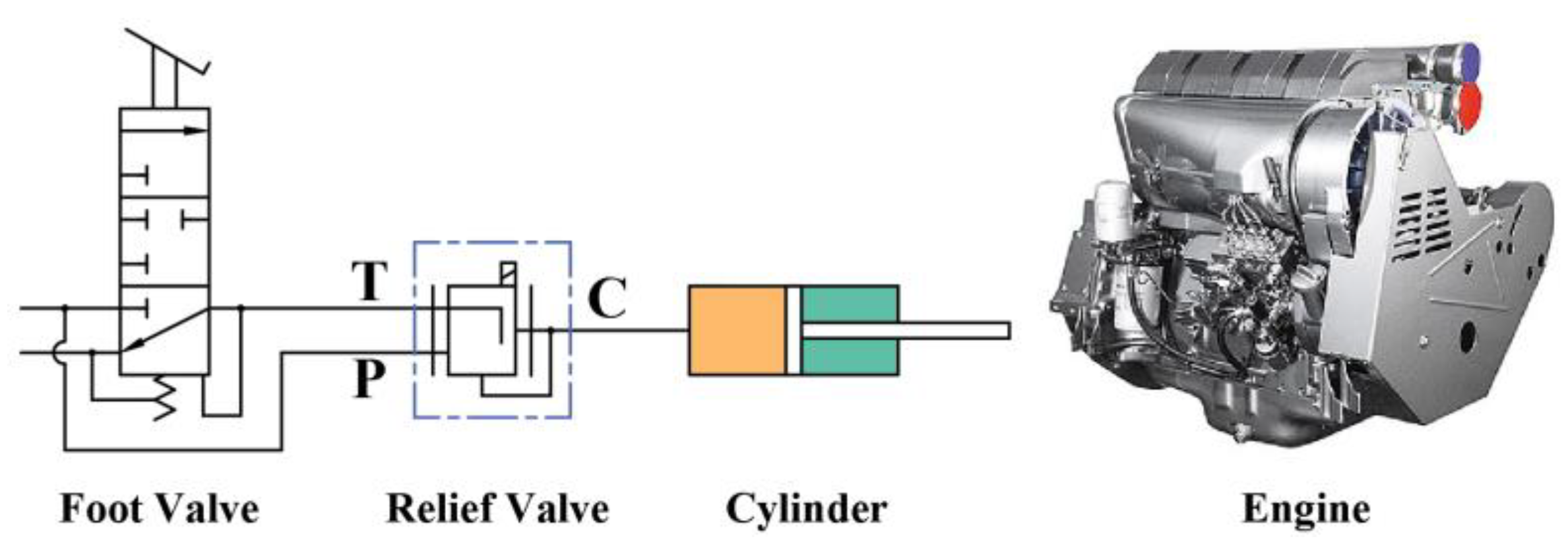
4.2. Driving-by-Wire System

The original throttle system is controlled by a hydraulic cylinder through a foot valve, which pushes a lever on the engine to control the throttle opening. An electronically controlled relief valve is equipped between the foot valve and the hydraulic cylinder for autonomous driving, as shown in Figure 10.

The original braking system already contains solenoid valves, which control the valves’ opening to achieve different braking efforts. Therefore, the vehicle’s braking can be controlled electronically by connecting the solenoid valve to the autonomous driving controller.

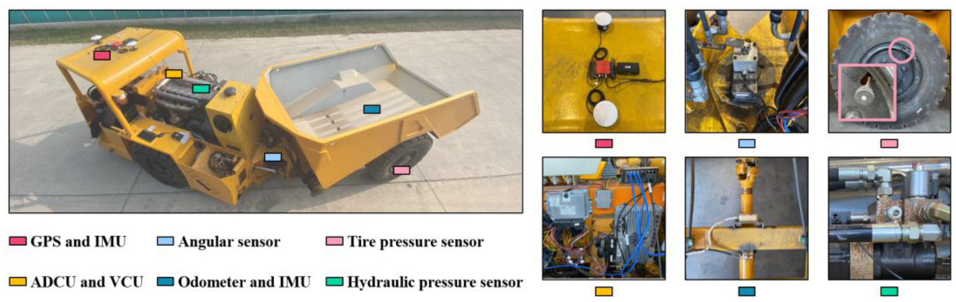
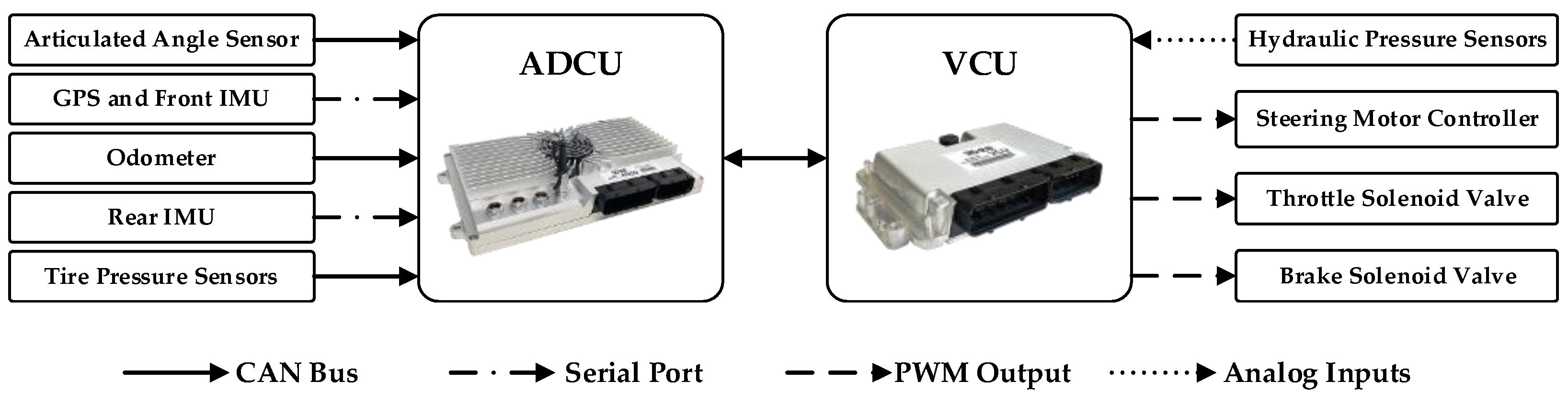
4.3. Sensors and Controllers

Figure 11 shows the installation layout of vehicle sensors and controllers in the actual vehicle test. An IMU and GPS fusion sensor, IFS2000, is equipped above the cab of the vehicle’s front body with an RTK positioning accuracy of 10 mm. The abovementioned steering-by-wire system is mounted on the right frame of the front body. KTGJ-CAN-S, the angle sensor, is mounted on the articulated center and used to measure the angle between the front and rear car body at 1000 Hz. On the rear body frame are SC12-20K gear speed sensor and XW-IMU5251F02 IMU, which measure the rear axle rotation speed and rear body acceleration, respectively. In addition, tire pressure sensors are installed on each wheel.

For controllers, an automated driving control unit (ADCU), EAXVA04, serves as an intelligent computing platform to receive and compute-intensive sensor data and perform fusion work, in which the path planning controller and path tracking controller are also integrated. The vehicle control unit (VCU), model EV2274A, acts as a controller to receive control outputs from the ADCU and convert them into control signals for each actuator.

The hardware architecture and communication between sensors, controllers, and actuators are shown in Figure 12. The GPS and IMU of front and rear vehicles input information to ADCU through the RS232 serial port. The ADCU receives information from the angle sensor, odometer, and tire pressure sensor through the CAN bus. The ADCU and VCU communicate with each other through the CAN bus. The VCU receives analog signals from the hydraulic pressure sensors. In addition, the VCU sends PWM waves to the steering motor controller, throttle actuator, brake actuator, and other actuators (e.g., dumping system and parking system).

5. Field Testing

5.1. Lower-Level Controller Verification

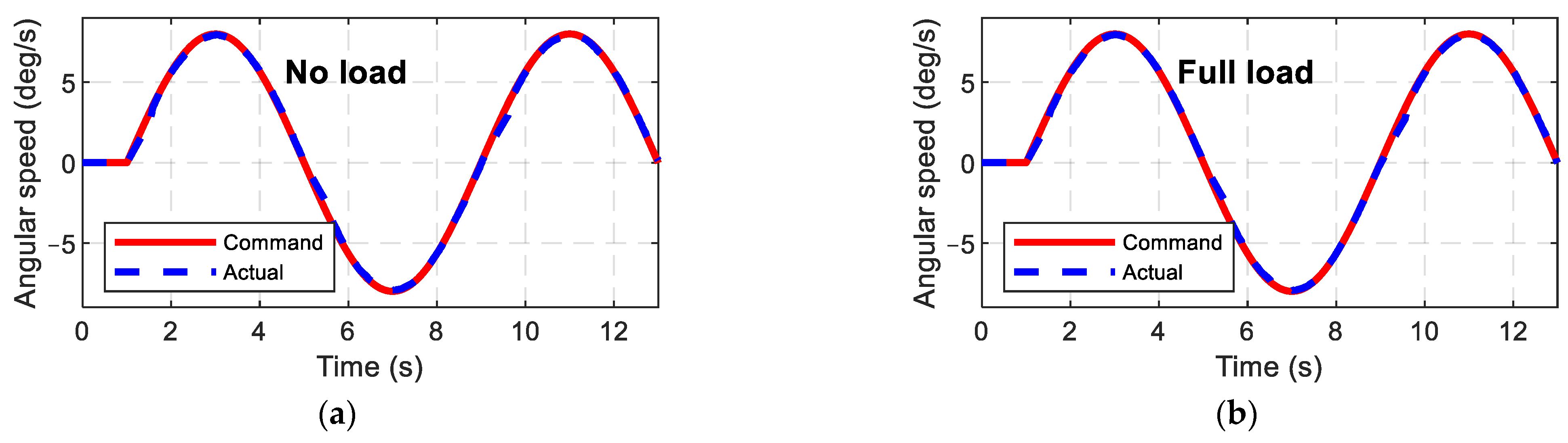
5.1.1. Steering Controller Verification

The articulated angular speed tracking experiments are performed under no-load and full-load conditions to verify the proposed steering controller. The reference articulated angular speed is a sinusoidal curve with a period of $T=8 \mathrm{s}$ and an amplitude of $8 \mathrm{degrees}$. The result indicates that the steering controller enables the vehicle to accurately track the desired articulated angular speed, as shown in Figure 13.

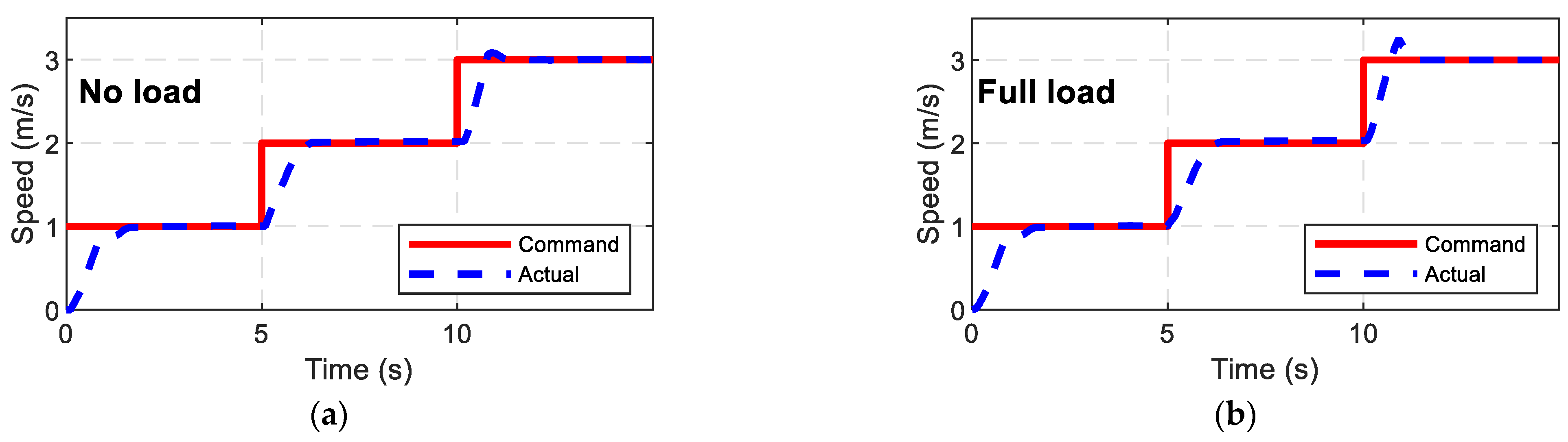
5.1.2. Driving Controller Verification

To validate the trained neural network, the speed tracking experiments are carried out under no-load and full-load conditions, respectively. In the experiments, the step desired speeds of $1 \mathrm{m}/\mathrm{s}$, $2 \mathrm{m}/\mathrm{s}$, and $3 \mathrm{m}/\mathrm{s}$ are given every five seconds. The experimental results are shown in Figure 14, where the vehicle tracks at the desired speed in a shorter time and maintains it afterward. In addition, it should be noted that the controller has undershoot performance at a desired speed of 1 m/s and some overshoot performance at a desired speed of 3 m/s. This is due to the fact that the entire drive system (including the extended engine, torque converter, and transmission) is a nonlinear system.

5.2. Integrated Path Tracking Controller Testing

In order to investigate the performance of the NMPC path tracking controller, the path tracking experiment of the articulated dump truck on a paved road is performed. As shown in Figure 15, the path tracking control system can be divided into three major subsystems: the vehicle (including sensors and actuators), the upper-level controller containing an extended Kalman filter (EKF) fusion positioning module and an NMPC path tracking controller, and the lower-level controller including load calculation module, the driving controller, and steering controller.

During the experiment, the vehicle’s GPS and front IMU provide the vehicle’s latitude, longitude, and heading in the geodetic coordinate system to the reference path module in the upper-level controller. The module outputs the local reference path for the NMPC path tracking controller. Meanwhile, the EKF module fuses the GPS and IMU data to calculate and output the vehicle status (the coordinates in the vehicle body coordinate system, the heading angle, and the current speed of the vehicle). The NMPC path tracking controller collects the data and computes the vehicle’s following control outputs (desired speed and desired steering rate). The upper-level controller broadcasts the outputs to the lower-level controller via the CAN bus. The load calculation module in the lower-level controller calculates the vehicle load based on the data from the IMU on the rear body and transmits the data to the driving controller. The driving and steering controllers in the lower-level control calculate the corresponding control commands and forward them to the vehicle’s actuators, respectively. After implying the commands, the sensors collect new information and perform the next tracking cycle.

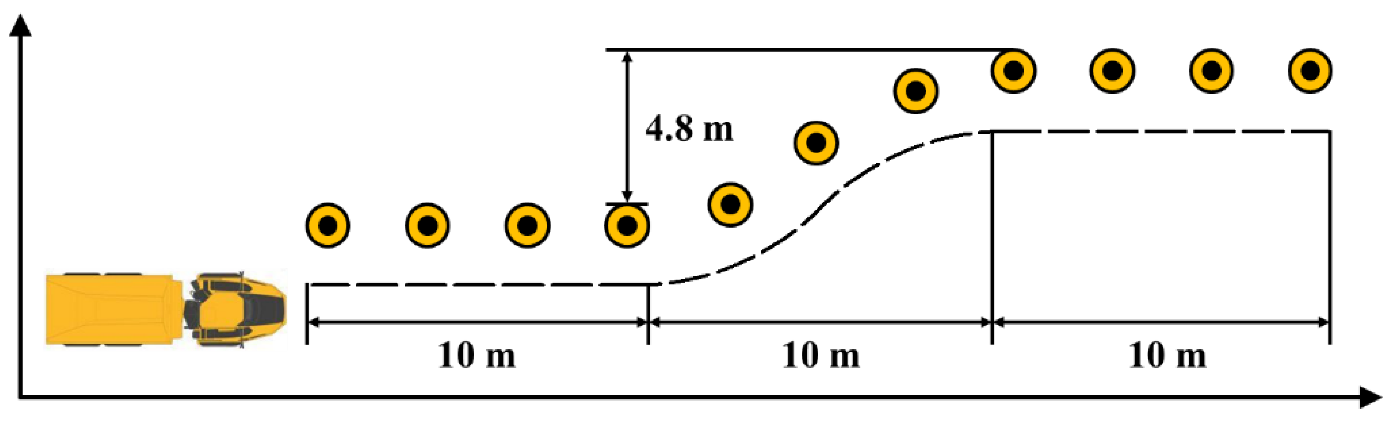
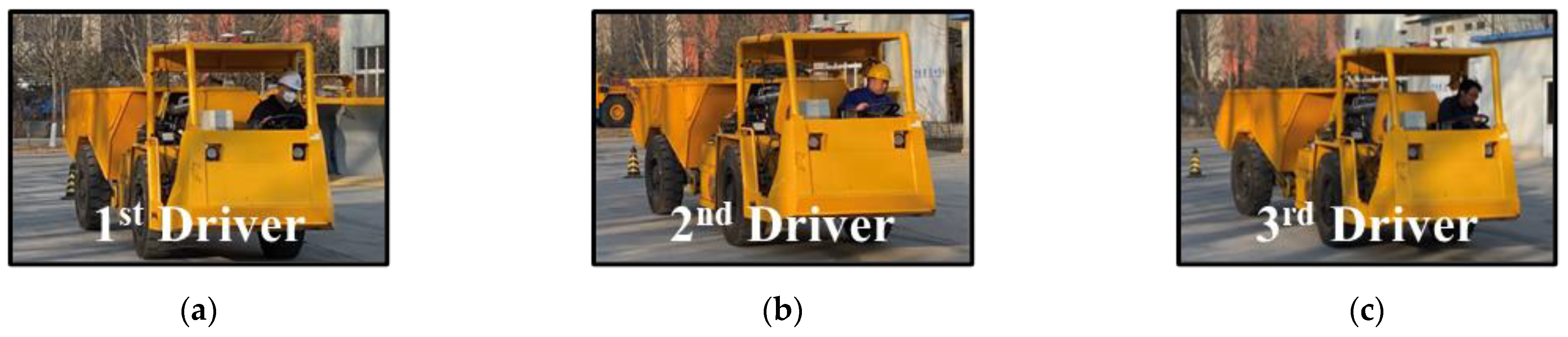
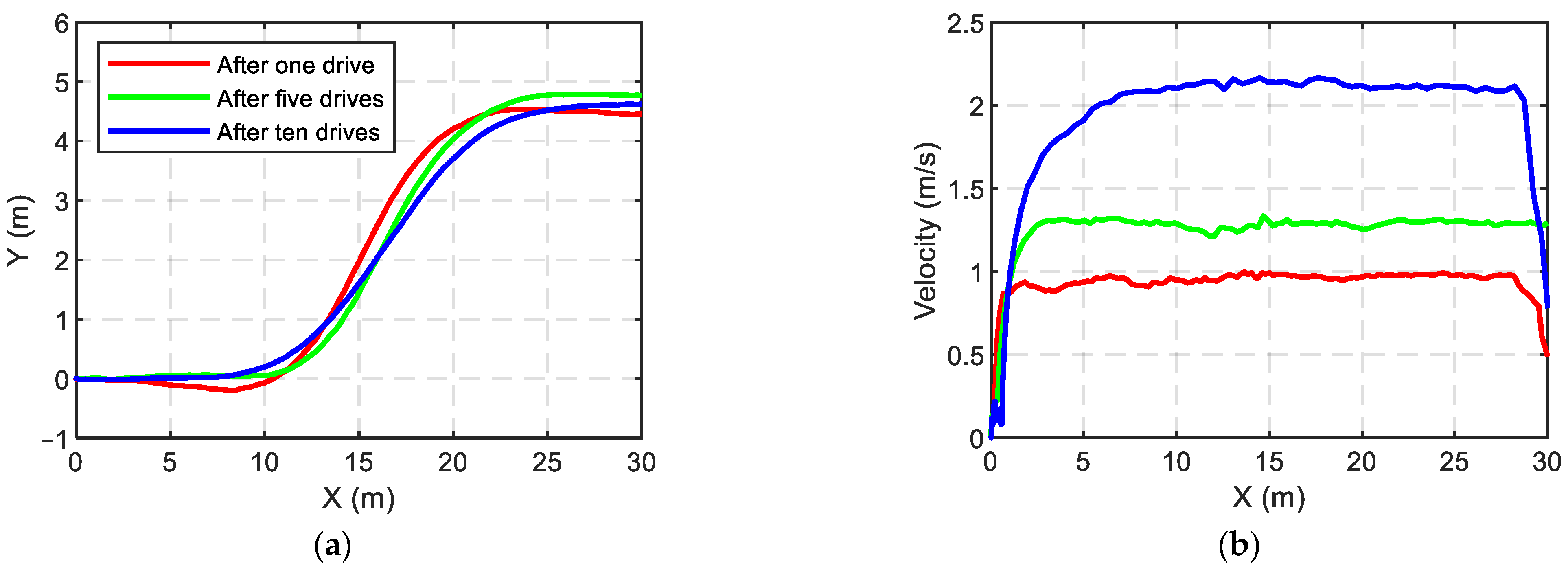
5.2.1. Pre-Experiment

With narrow roads and complex road conditions in the underground tunnels, surface experiments are conducted at the vehicle’s manufacturing factory in order to ensure safety. The experimental site is shown in Figure 16, and the maximum available road width is 10 m. The width is similar to the roadway path of the underground metal mine.

In this width condition, vehicle meeting and obstacle avoidance happen frequently. Therefore, a single shift line is selected as the reference path. Road cones are placed as a reference, as shown in Figure 17. The path is divided into three longitudinal sections of $10 \mathrm{m}$ each, with the first $10 \mathrm{m}$ being the acceleration section, the middle $10 \mathrm{m}$ being the shift line section, and the subsequent section to ensure the vehicle is driven straight. The lateral spacing of the shift line section is set to $4.8 \mathrm{m}$.

Before path tracking, a speed test with artificial driving is performed. It is designed to identify the maximum speed that can be driven under this path so that the path tracking experiment can avoid dangerous conditions such as a rollover.

As shown in Figure 18, three drivers participated in the experiment, and each driver drives ten times at the highest speed according to the reference path based on their driving ability. The highest speed is taken as the result.

The results are shown in Figure 19. The maximum speed after one drive is $1 \mathrm{m}/\mathrm{s}$. After five drives, the maximum speed is $1.3 \mathrm{m}/\mathrm{s}$. After ten drives, the maximum speed is $2.1 \mathrm{m}/\mathrm{s}$.

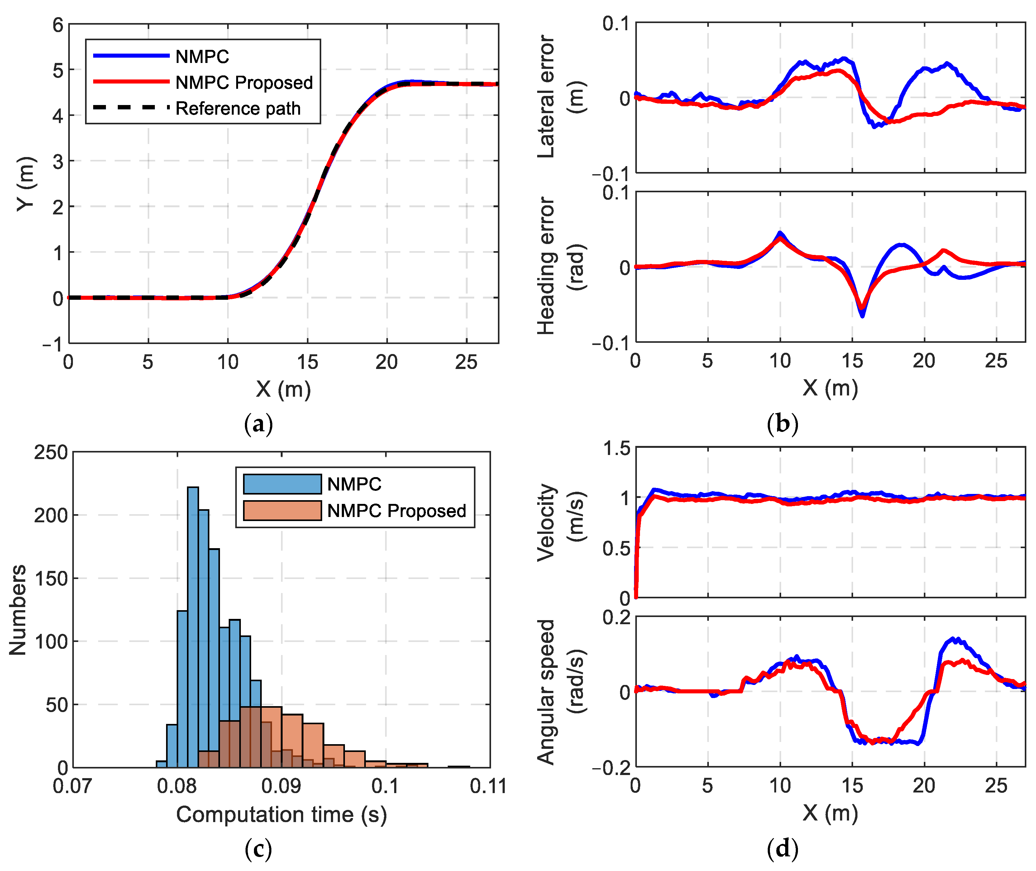
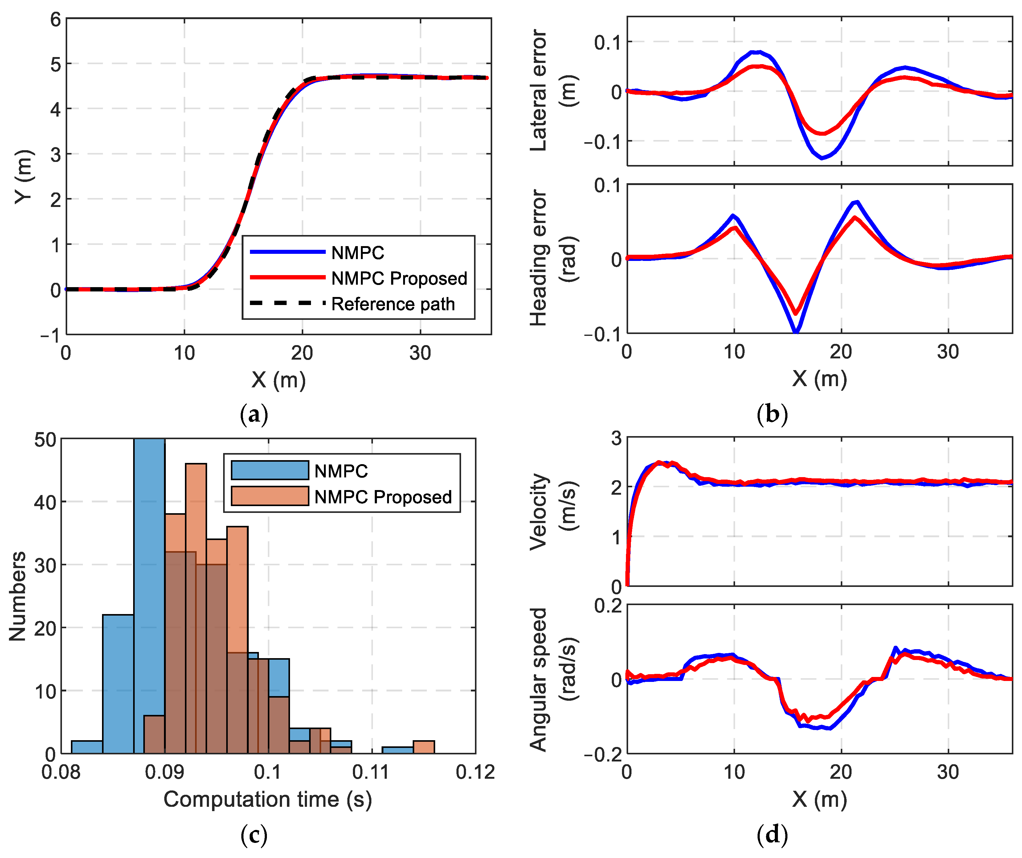
5.2.2. Tracking Result

According to the pre-experiment results, the reference speed is set to $1 \mathrm{m}/\mathrm{s}$ and $2 \mathrm{m}/\mathrm{s}$. The controller is tested under each reference speed and unloaded condition, respectively. The parameters of the integrated path tracking controller in the experiment are shown in

Table 2. Parameters of NMPC path tracking controller.

Parameters	Value
$N_{\mathrm{p}}$	20
$N_{\mathrm{c}}$	$10$
$T$	$0.1\mathrm{s}$
$P$	$\mathrm{diag}\left(0.1, 0.1, 0.5, 0\right)\in {ℝ}^{4\times 4}$
$Q$	$\mathrm{diag}\left(0.01, 0.01, 0.05, 0\right)\in {ℝ}^{4\times 4}$
$R$	$\mathrm{diag}\left(0.01, 0.01\right)\in {ℝ}^{2\times 2}$
${\gamma }_{\min },{\gamma }_{\max }$	$-0.73\mathrm{rad},0.73\mathrm{rad}$
$v_{\min },v_{\max }$	$0\mathrm{m}/\mathrm{s},4\mathrm{m}/\mathrm{s}$
${\mathsf{\omega }}_{\min },{\mathsf{\omega }}_{\max }$	$-0.17\mathrm{rad}/s,0.17\mathrm{rad}/s$
$\mathsf{\Delta }{v}_{\min },\mathsf{\Delta }{v}_{\max }$	$-0.3\mathrm{m}/{\mathrm{s}}^2,0.3\mathrm{m}/{\mathrm{s}}^2$
$\mathsf{\Delta }{\mathsf{\omega }}_{\min },\mathsf{\Delta }{\mathsf{\omega }}_{\max }$	$-0.17\mathrm{rad}/{\mathrm{s}}^2,0.17\mathrm{rad}/{\mathrm{s}}^2$

. The parameters are chosen based on the summary of numerous experimental results. According to Equation (7), the larger $N_{\mathrm{p}}$ has a minor overall error between the tracking path and the reference path, but the error becomes more significant in the path in which the curvature changes significantly, and an excessive $N_{\mathrm{p}}$ leads to computational stress. Similarly, the error is smaller when $N_{\mathrm{c}}$ gradually increases to $N_{\mathrm{p}}$, but an oversized $N_{\mathrm{c}}$ causes more computational stress than excessive $N_{\mathrm{p}}$. Therefore, according to the experimental experience, $N_{\mathrm{p}}$ is chosen to be 20 and $N_{\mathrm{c}}$ to be 10. Q, $R$, and $P$ are mainly responsible for adjusting the weight values among the cost functions to make them consistent in scale. However, an overly large weight will increase the computational load. Thus, they should be as small as possible without exceeding the minimum accuracy of the solver. The weights in the table are based on the experimental results to obtain the optimal relative values. CasADi is used as nonlinear optimization algorithm in this paper [15].

(a) Path Tracking Results at 1 m/s.

The experimental results are shown in Figure 20. The blue curve represents the controller with traditional NMPC, and the red curve represents the controller with NMPC with terminal cost. The results show that the integrated controller with both traditional NMPC and proposed NMPC can make the vehicle track the path. In the case of the traditional NMPC, the peak lateral error is 0.0518 m, and the peak heading angle error is 0.0659 rad. At the proposed NMPC, the peak lateral error is $0.0358 \mathrm{m},$ and the peak heading angle error is 0.0547 rad. It is evident that the NMPC controller with terminal cost can increase tracking accuracy and stabilize earlier. At the same time, in both cases, the vehicle speed is well controlled at the reference speed, and both the speed and the articulated angular speed change smoothly. The calculation time of the controller is concentrated on $0.08 \mathrm{s}$ to $0.09 \mathrm{s}$, and only a little exceeds $0.1 \mathrm{s}$ (the time interval of the controller); however, the computation time of NMPC with the terminal cost is slightly higher than that of traditional NMPC.

In summary, the integrated path tracking controller can ensure the vehicle path tracking at $1 \mathrm{m}/\mathrm{s}$ within reasonable accuracy.

(b) Path Tracking Results at 2 m/s.

The results show that both controllers can make the vehicle track the path. As shown in Figure 21, the peak lateral error is $0.1351\mathrm{m},$ and the peak heading angle error is $0.1014\mathrm{rad}$ under traditional NMPC. For the proposed NMPC, the peak lateral error is $0.0858 \mathrm{m}$, and the peak heading angle error is $0.0740\mathrm{rad}$. However, each peak error increases slightly compared to the reference speed of $1 \mathrm{m}/\mathrm{s}$. In addition, the lateral error in the traditional NMPC is slightly larger than that in the proposed NMPC case at the exact coordinates during the entire path tracking process. In both cases, the vehicle velocity is well controlled at the reference speed. Both the velocity and the steering rate are smooth. The computation time of the controller is concentrated around $0.09\mathrm{s}$, only very few times exceed $0.1$ s, which had no impact on the actual control; however, the computation time increases compared with the tracking result of 1 m/s.

In summary, the NMPC controller can guarantee vehicle path tracking at $2\mathrm{m}/\mathrm{s}$. As the velocity increases, however, the tracking error increases slightly, and the computation time rises marginally.

6. Conclusions

This paper introduces an integrated path controller consisting of an upper-level controller and a lower-level controller. The upper-level controller is the NMPC with a terminal-cost state tracking controller, which provides the upcoming longitudinal velocity and steering rate for path tracking. To meet the requirements of the upper-level controller, a lower-level controller is proposed, which includes a steering controller and a driving controller.

Verification experiments were conducted to validate the lower-level controller. The results demonstrate that the lower-level controller can accurately and rapidly achieve the desired longitudinal velocity and steering rate.

Path tracking experiments on a single shift line were performed using the integrated controller. The results indicate that the vehicles can precisely follow the reference path at different reference velocities. However, the controller with the terminal cost is more accurate and stable. The controllers’ solution times are all guaranteed to be less than the control time interval. However, as the reference velocity increases, both the peak lateral error and the peak heading angle error increase, and the solution time of the controller also increases.

This paper presents several significant contributions in the field of vehicle path tracking control.

(1) A novel method for controlling the articulated angular speed of the vehicle is proposed. Specifically, a stepper-motor-controlled fully hydraulic steering gear is employed to achieve wire control. Compared with the traditional solenoid-proportional directional valve, this control method exhibits no dead zone of steering speed, thus enabling the controller to achieve smaller steering speed. Furthermore, the coupling relationship between the engine, hydraulic oil pump, and solenoid proportional directional valve is decoupled, leading to simpler and more accurate steering control.

(2) A driving controller is developed using a BP neural network approach. The proposed controller is capable of ensuring that the vehicle can meet desired speeds for different loadings, surpassing other drive control algorithms in terms of performance.

(3) A terminal penalty cost is introduced into the NMPC controller, which significantly enhances the stability of the controller and reduces path tracking errors. Building upon this study, future research will focus on improving the stability and robustness of the NMPC. Additionally, machine learning algorithms will be utilized to enhance the prediction model’s accuracy and adaptability.

References

1. Altafini, C. Why to use an articulated vehicle in underground mining operations? In Proceedings of the 1999 IEEE International Conference on Robotics and Automation (Cat. No. 99CH36288C), Detroit, MI, USA, 10–15 May 1999; pp. 3020–3025. [Google Scholar]
2. Rowduru, S.; Kumar, N.; Kumar, A. A critical review on automation of steering mechanism of load haul dump machine. Proc. Inst. Mech. Eng. Part I J. Syst. Control Eng. 2020, 234, 160–182. [Google Scholar] [CrossRef]
3. Cai, M.; Xue, D.; Ren, F. Current status and development strategy of metal mines. Chin. J. Eng. 2019, 41, 417–426. [Google Scholar]
4. Cai, M.; Li, P.; Tan, W.; Ren, F. Key Engineering Technologies to Achieve Green, Intelligent, and Sustainable Development of Deep Metal Mines in China. Engineering 2021, 7, 1513–1517. [Google Scholar] [CrossRef]
5. Ardiny, H.; Witwicki, S.; Mondada, F. Construction automation with autonomous mobile robots: A review. In Proceedings of the 2015 3rd RSI International Conference on Robotics and Mechatronics (ICROM), Tehran, Iran, 7–9 October 2015; pp. 418–424. [Google Scholar]
6. Amer, N.H.; Zamzuri, H.; Hudha, K.; Kadir, Z.A. Modelling and control strategies in path tracking control for autonomous ground vehicles: A review of state of the art and challenges. J. Intell. Robot. Syst. 2017, 86, 225–254. [Google Scholar] [CrossRef]
7. Xu, S.; Peng, H. Design, analysis, and experiments of preview path tracking control for autonomous vehicles. IEEE Trans. Intell. Transp. Syst. 2019, 21, 48–58. [Google Scholar] [CrossRef]
8. Yao, Q.; Tian, Y.; Wang, Q.; Wang, S. Control strategies on path tracking for autonomous vehicle: State of the art and future challenges. IEEE Access 2020, 8, 161211–161222. [Google Scholar] [CrossRef]
9. Rokonuzzaman, M.; Mohajer, N.; Nahavandi, S.; Mohamed, S. Review and performance evaluation of path tracking controllers of autonomous vehicles. IET Intell. Transp. Syst. 2021, 15, 646–670. [Google Scholar] [CrossRef]
10. Ji, J.; Khajepour, A.; Melek, W.W.; Huang, Y. Path planning and tracking for vehicle collision avoidance based on model predictive control with multiconstraints. IEEE Trans. Veh. Technol. 2016, 66, 952–964. [Google Scholar] [CrossRef]
11. Falcone, P.; Borrelli, F.; Asgari, J.; Tseng, H.E.; Hrovat, D. Predictive active steering control for autonomous vehicle systems. IEEE Trans. Control Syst. Technol. 2007, 15, 566–580. [Google Scholar] [CrossRef]
12. Gong, J.; Xu, W.; Jiang, Y.; Liu, K.; Guo, H.; Sun, Y. Multi-constrained model predictive control for autonomous ground vehicle trajectory tracking. J. Beijing Inst. Technol. 2015, 24, 441–448. [Google Scholar]
13. Bai, G.; Meng, Y.; Liu, L.; Luo, W.; Gu, Q.; Liu, L. Review and comparison of path tracking based on model predictive control. Electronics 2019, 8, 1077. [Google Scholar] [CrossRef]
14. Matschek, J.; Bäthge, T.; Faulwasser, T.; Findeisen, R. Nonlinear predictive control for trajectory tracking and path following: An introduction and perspective. In Handbook of Model Predictive Control; Springer: Cham, Switzerland, 2019; pp. 169–198. [Google Scholar]
15. Andersson, J.A.; Gillis, J.; Horn, G.; Rawlings, J.B.; Diehl, M. CasADi: A software framework for nonlinear optimization and optimal control. Math. Program. Comput. 2019, 11, 1–36. [Google Scholar] [CrossRef]
16. Nayl, T.; Nikolakopoulos, G.; Gustfsson, T. Switching model predictive control for an articulated vehicle under varying slip angle. In Proceedings of the 2012 20th Mediterranean Conference on Control & Automation (MED), Barcelona, Spain, 3–6 July 2012; pp. 890–895. [Google Scholar]
17. Nayl, T.; Nikolakopoulos, G.; Gustafsson, T. A full error dynamics switching modeling and control scheme for an articulated vehicle. Int. J. Control Autom. Syst. 2015, 13, 1221–1232. [Google Scholar] [CrossRef]
18. Dou, F.; Huang, Y.; Liu, L.; Wang, H.; Meng, Y.; Zhao, L. Path planning and tracking for autonomous mining articulated vehicles. Int. J. Heavy Veh. Syst. 2019, 26, 315–333. [Google Scholar] [CrossRef]
19. Bai, G.; Liu, L.; Meng, Y.; Luo, W.; Gu, Q.; Ma, B. Path tracking of mining vehicles based on nonlinear model predictive control. Appl. Sci. 2019, 9, 1372. [Google Scholar] [CrossRef]
20. Gao, L.; Jin, C.; Liu, Y.; Ma, F.; Feng, Z. A Novel Model-Based Steering Control for Hydra-Power Articulated Steering Vehicles. In Proceedings of the BATH/ASME 2020 Symposium on Fluid Power and Motion Control, Virtual, 9–11 September 2020; ASME: New York, NY, USA, 2020; p. V001T001A006. [Google Scholar]
21. Nelson, F.W.; Pickett, T.D. Vehicle Guidance System with a Stepper Motor. US9834248B2, 15 January 2016. [Google Scholar]
22. Liu, J.; Tan, J.; Mao, E.; Song, Z.; Zhu, Z. Proportional directional valve based automatic steering system for tractors. Front. Inf. Technol. Electron. Eng. 2016, 17, 458–464. [Google Scholar] [CrossRef]
23. Daher, N.; Ivantysynova, M. Energy analysis of an original steering technology that saves fuel and boosts efficiency. Energy Convers. Manag. 2014, 86, 1059–1068. [Google Scholar] [CrossRef]
24. Jangnoi, T.; Pinsopon, U. Velocity control of electro-hydraulic pump control system using gear pump. Int. J. Innov. Comput. Inf. Control 2018, 14, 2307–2323. [Google Scholar]
25. Liu, W.; Xia, X.; Xiong, L.; Lu, Y.; Gao, L.; Yu, Z. Automated vehicle sideslip angle estimation considering signal measurement characteristic. IEEE Sens. J. 2021, 21, 21675–21687. [Google Scholar] [CrossRef]
26. Zhao, X.; Yang, J.; Zhang, W.; Zeng, J. Feedback linearization control for path tracking of articulated dump truck. TELKOMNIKA Telecommun. Comput. Electron. Control 2015, 13, 922–929. [Google Scholar] [CrossRef]
27. Borrelli, F.; Bemporad, A.; Morari, M. Predictive Control for Linear and Hybrid Systems; Cambridge University Press: Cambridge, UK, 2017. [Google Scholar]
28. Zhu, F.; Ma, L.; Xu, X.; Guo, D.; Cui, X.; Kong, Q. Baidu apollo auto-calibration system-an industry-level data-driven and learning based vehicle longitude dynamic calibrating algorithm. arXiv 2018, arXiv:1808.10134. [Google Scholar]
29. Haddoun, A.; Benbouzid, M.E.H.; Diallo, D.; Abdessemed, R.; Ghouili, J.; Srairi, K. Modeling, analysis, and neural network control of an EV electrical differential. IEEE Trans. Ind. Electron. 2008, 55, 2286–2294. [Google Scholar] [CrossRef]
Figure 1. Diagram of the NMPC path tracking process.
Applsci 13 05340 g001
Figure 2. Kinematic model of underground mining articulated vehicle.
Applsci 13 05340 g002
Figure 3. Articulated steering structure motion sketch.
Applsci 13 05340 g003
Figure 4. Relationship between articulated angle, control command, and articulated angular speed: (a) left turn; (b) right turn.
Applsci 13 05340 g004
Figure 5. Neural networks for speed control.
Applsci 13 05340 g005
Figure 6. Articulated dump truck with no-load condition and full-load condition: (a) no load; (b) full load.
Applsci 13 05340 g006
Figure 7. Articulated dump truck configuration.
Applsci 13 05340 g007
Figure 8. Steering-by-wire system hydraulic schematic.
Applsci 13 05340 g008
Figure 9. Steering-by-wire system on vehicle.
Applsci 13 05340 g009
Figure 10. Driving-by-wire system.
Applsci 13 05340 g010
Figure 11. The installation layout of sensors and controllers on the vehicle body.
Applsci 13 05340 g011
Figure 12. The layout of hardware architecture and communication.
Applsci 13 05340 g012
Figure 13. Experimental verification results of steering controller: (a) no load; (b) full load.
Applsci 13 05340 g013
Figure 14. Experimental verification results of driving controller: (a) no load; (b) full load.
Applsci 13 05340 g014
Figure 15. Diagram of articulated dump truck path tracking system.
Applsci 13 05340 g015
Figure 16. Path tracking experimental site: (a) top view of the site; (b) road surface of the site.
Applsci 13 05340 g016
Figure 17. Diagram of artificial reference cones’ placement.
Applsci 13 05340 g017
Figure 18. Three drivers in the maximum speed test: (a) 1st driver; (b) 2nd driver; (c) 3rd driver.
Applsci 13 05340 g018
Figure 19. Speed test results: (a) path comparison results; (b) velocity comparison results.
Applsci 13 05340 g019
Figure 20. Path tracking results at 1 m/s: (a) path comparison results; (b) lateral error and heading error comparison results; (c) computation time comparison results; (d) control inputs comparison results.
Applsci 13 05340 g020
Figure 21. Path tracking results at 2 m/s: (a) path comparison results; (b) lateral error and heading error comparison results; (c) computation time comparison results; (d) control inputs comparison results.
Applsci 13 05340 g021