Article

Multi-Source HRRP Target Fusion Recognition Based on Time-Step Correlation

School of Electronic Engineering, Naval University of Engineering, Wuhan 430033, China
*
Author to whom correspondence should be addressed.
Appl. Sci. 2023, 13(9), 5286; https://doi.org/10.3390/app13095286
Submission received: 17 March 2023 / Revised: 10 April 2023 / Accepted: 20 April 2023 / Published: 23 April 2023

Abstract

:
Aiming at the limitations of a single High Resolution Range Profile (HRRP) in recognition, this paper proposes a Time step Correlation-based Feature Fusion (TCFF) method. This method calculates the covariance matrix at the time step of the two features extracted by the two channels, and assigns different weights to the time step according to the strength of the covariance correlation for feature fusion. The experimental results on the simulated ship target HRRP dataset show that the feature fusion method can achieve better recognition performance than the single channel model. Compared with simple feature fusion such as element addition and element contacting, it can also achieve better recognition results.

1. Introduction

The high-resolution range profile is a one-dimensional projection of target scattering points along the radar line of sight. It contains rich information such as target scattering fluctuation characteristics, geometry, and attitude. Compared with SAR images, HRRP is easy to obtain, store and process quickly [1]. Therefore, using the HRRP for target recognition has attracted wide attention in the field of RATR [1,2,3,4,5,6,7,8,9,10].
Extracting stable and easily distinguishable features from HRRP data is the key technique of RATR, which has become a research hotspot for domestic and foreign scholars. Zhang et al. [1], Liao et al. [2] and Du et al. [11] started from the spectrum of the HRRP to extract features that are easy to identify. The recognition accuracy of these methods largely depends on manual extraction of spectral features, which is not conducive to engineering promotion. In order to weaken the influence of this artificial factor, Du et al. [12] applied Principal Component Analysis (PCA) to extract HRRP features by minimizing reconstruction errors. Feng et al. [13] used dictionary learning to approximate sparse signals to extract HRRP features. Pan et al. [14] proposed a radar HRRP model based on a hidden Markov model, combined with time domain features and spectral features, and achieved good results.
In recent years, the rapid development of deep learning has provided a new approach for radar automatic target recognition. Extracting stable features that are easy to distinguish from HRRP data through neural networks and machine learning algorithms has become a popular research direction. The literature [15,16,17] used RNNs in recurrent neural networks, Long Short-Term Memory (LSTM), and a Gated Recurrent Unit (GRU) to classify HRRP targets and combined them with attention mechanisms to achieve good results. The literature [18] used a Convolutional Neural Network (CNN) to construct a deep model for classification and rejection of HRRP targets by convolution and deconvolution operations on convolutional kernels of different sizes. [9], a Stacked Corrective Autoencoder (SCAE) is proposed on the basis of a Stacked Autoencoder (SAE), and through a series of stacked Corrective Autoencoders (CAEs). The recognition effect of HRRP is improved by stacking a series of Corrective Autoencoders (CAEs). All of the above methods use a single HRRP for target classification, and the quality of the data directly affects the effectiveness of recognition. In today’s modern warfare, the use of different radars to collaborate on target recognition is the trend of early warning detection system development, and multi-source target fusion recognition has been developed in this context.
Multi-source target fusion methods are divided into decision-level fusion methods and feature-level fusion methods. The decision-level fusion methods are as follows: the literature [19] uses the decision template of each target obtained by training, compares the decision results of the sample with the decision templates of various targets, and determines the target category by similarity. The literature [20,21] introduced the decision-level fusion recognition method based on the D-S evidence theory, and further improved the traditional D-S theory based on the discount principle to make it more suitable for radar target data. The feature-level fusion methods are as follows: the literature [22] fuses several typical features of low-resolution radar and classifies targets by a Support Vector Machine (SVM). Refs. [23,24], a fusion algorithm based on Canonical Correlation Analysis (CCA) is used to select features by correlation size, which not only retains the useful information of the target, but also eliminates redundant information, and realizes the effective fusion of multiple features. Refs. [24,25], a Stacked Autoencoder and a Deep Convolutional Neural Network (DCNN) dual-channel network, a bidirectional LSTM and a bidirectional GRU dual-channel network were constructed, respectively, and the dual-channel extraction features were spliced and fused. Finally, the recognition effect was significantly improved through the classification of a fully connected layer and a SoftMax layer.
Aimed at the timing characteristics of HRRP, this paper proposes a Time-step Correlation-based Feature Fusion (TCFF) module. The module uses the temporal characteristics of the HRRP to assign weights to the multi-source features extracted by the feature extraction module according to the time-step correlation strength and performs feature fusion. Finally, the SoftMax classifier achieves target classification. Compared with the simple element addition and element splicing fusion method, it avoids information redundancy and makes better use of the useful information contained in the HRRP. The effectiveness of the TCFF fusion method is verified by experiments in different feature extraction modules.

2. Proposed Model

2.1. Multi-Source Feature Fusion Recognition Network Based on Time-Tep Correlation

A Time-step Correlation-based Feature Fusion (TCFF) model is proposed and combined with the traditional neural network model in this paper. The model uses dual-channel input, and the obtained different HRRP is pre-processed and input into the same feature extraction network to extract deep and easily distinguishable features. According to the correlation between different time steps of the HRRP, the features under different time steps are weighted, and the strong correlation is given higher weights to make better use of the useful information of the target and avoid the adverse effects of redundant information on target recognition. The model structure diagram is shown in Figure 1.

2.2. Data Pre-Processing

Due to the varying cross-sectional area of scattering at different positions of the target, the amplitude of the echo signal received by the radar varies greatly. The raw HRRP data of the target has amplitude sensitivity [26,27], which can have a significant impact on the recognition performance of the model. Therefore, this paper performs 2-norm normalization on the HRRP of the original ship target to eliminate amplitude sensitivity and improve the recognition effect of the model on the HRRP. Assuming that the expression of the original HRRP data after normalization is:
p = p 1 , p 2 , . . . , p N T
where N is the number of distance units and pi is the normalized amplitude of the ith distance unit.
In this paper, the sliding window method is used to convert the HRRP data after amplitude normalization into sequence data [27]. Assuming the existence of a window with a width of d, the HRRP data after amplitude normalization is intercepted into sequence data by sliding the set window in fixed steps, assuming that each sliding distance is c. The HRRP after sliding the window can be expressed as
X = x 1 , x 2 , . . , x T
x l = p l 1 c + 1 , p l 1 c + 2 , . . . , p l 1 c + d
where x l R d × 1 is the input at moment l. In the vector X R d × T , T represents T time steps and d represents the sequence length of each time step as d.

2.3. Feature Extraction Network

In order to verify the effectiveness of the feature fusion method, seven feature extraction networks are selected in this paper, which are Recurrent Neural Networks (RNNs), LSTM [28], GRU [29], Simple Recurrent Units (SRUs) [30], encoder part in Transformer [31], R-Transformer [32] and R-DeLighT [32] models. This section introduces the R-DeLighT model, whose structure is shown in Figure 2. The model is mainly composed of a local RNN module and a Transformer-Encoder feature extraction module that introduces Group Linear Transformations (GLTs).
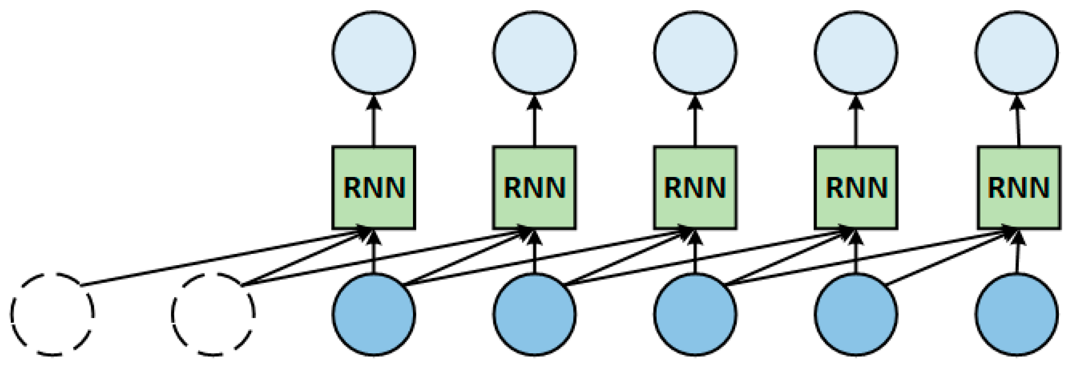
The local RNN module consists of parallel RNN modules designed to take full advantage of RNN in extracting short sequence signal features. The structure of the local RNN module is shown in Figure 3 [32].
Figure 3 shows the local RNN module structure when the window size of the sliding window is 3. For a more general explanation, we assume that the window size of the sliding window in the local RNN module is k. A new input sequence X is formed by adding k −1 zero sequences of the same size in time steps to the left side of the original input x :
X = 0 , . . . k 1 , 0 , x 1 , x 2 , . . . , x T
The sliding window with a size of k is slid from left to right, and the sliding distance is 1. Then T short sequences are formed, and the hidden state vectors output by T RNN are spliced into new hidden state vectors.
h t = R N N x t k + 1 , x t k + 2 , . . . , x t
H = h 1 , h 2 , . . . , h T
where h t is the output of the hidden layer vector in the t-th RNN. R N N is a simplification of the RNN principal formula.
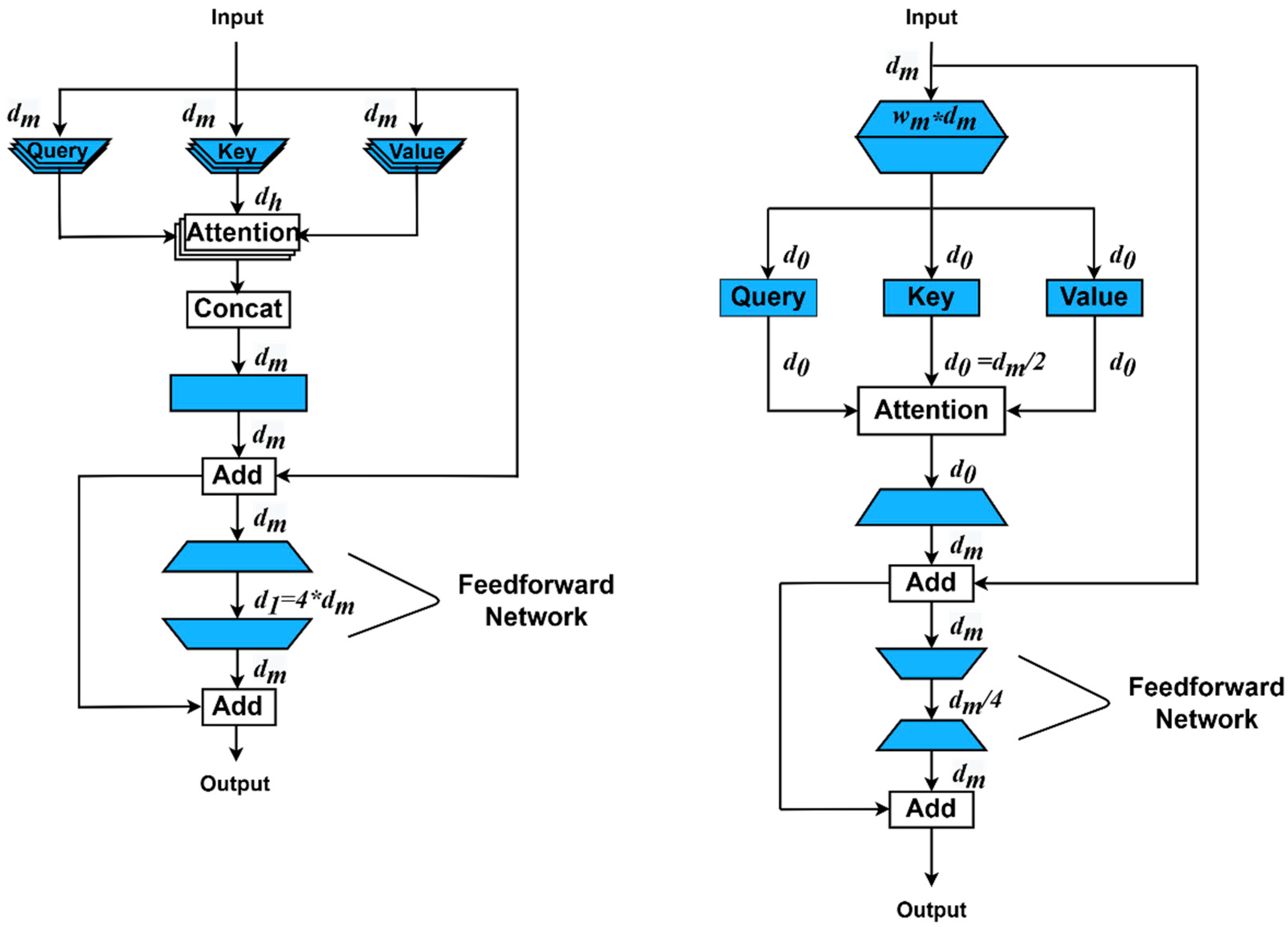
The GLTs are introduced into the Transformer model encoder structure to improve the model recognition performance while reducing the model parameters. Comparison of standard Transformer model encoder structure (left) and Transformer model encoder structure combined with GLTs is shown in Figure 4 [32].
The module first takes the hidden layer vector H output by the local RNN module as the input of the model. Assuming there are N layers of GLTs in this module. The modules of GLTs have two stages: expansion stage and reduction stage. In the expansion stage, in N / 2 linear layer, the input of dimension d m is projected onto a high-dimensional space of dimension d max . where d max = w m d m , and w m is the expansion coefficients. Similarly, in the reduction stage, use the remaining N N / 2 layers to project the d m a x dimensional vector onto the d 0 dimensional vector.
g l = min 2 l 1 , g m a x , 1 l N / 2 g N l , otherwise
where g max is the set maximum number of linear transformation layers per layer. g l denotes the number of linear transformation layers contained in the lth layer.
Y l = F H , W l , b l , g l , l = 1 F M I X H , Y l 1 , W l , b l , g l , o t h e r w i s e
where W l = [ W 1 l , W 2 l , . . . , W g l l ] and b l = b 1 l , b 2 l , . . . , b g l l are the weights and bias of the g l group linear transformation function in the lth layer, respectively. F is a linear transformation function that divides the input H into g l non-overlapping groups so that H can be written as H = H 1 , H 2 , . . . , H g l , and the linear layer transforms each H i by the weights W i l and b i l to obtain an output Y i l = H i W i l + b i l . The output Y i l of each group is then stitched to produce the final output Y l .
The GLTs module concatenates the output vector Y l 1 of layer l−1 with input H through a mixer and disrupts the order. Input it into the linear layer to extract more stable features of the target. The calculation process of the mixer is as follows:
M I X H , Y l 1 = shuffle H , Y l 1
where shuffle is the random grouping of the input features and the output after stitching. Taking the linear transform group with three layers in the upscaling stage as an example, the workflow of the mixer is shown in Figure 5.
Because of the superior performance of GLTs, the Self-Attention module is used instead of the Multi-Head attention module:
u t = Sel f attention Y l = Attention Q , K , V = softmax Q K T d k
where Q, K, and V are obtained by linear transformation of vector Y l .
After completing the calculation of attention, the next module is the lightweight feedforward neural network layer. This module contains two linear transformation layers and one nonlinear layer to transform the input feature vectors. In this module, the activation function of the nonlinear layer uses the GELU function, and the dimension transformation of the linear transformation layer is first reduced and then expanse:
v = Feedforward u = u W 1 + b 1 ϕ u W 1 + b 1 W 2 + b 2
where ϕ x is the cumulative distribution function of the normal distribution.

2.4. Time-Step Correlation-Based Feature Fusion (TCFF) Module

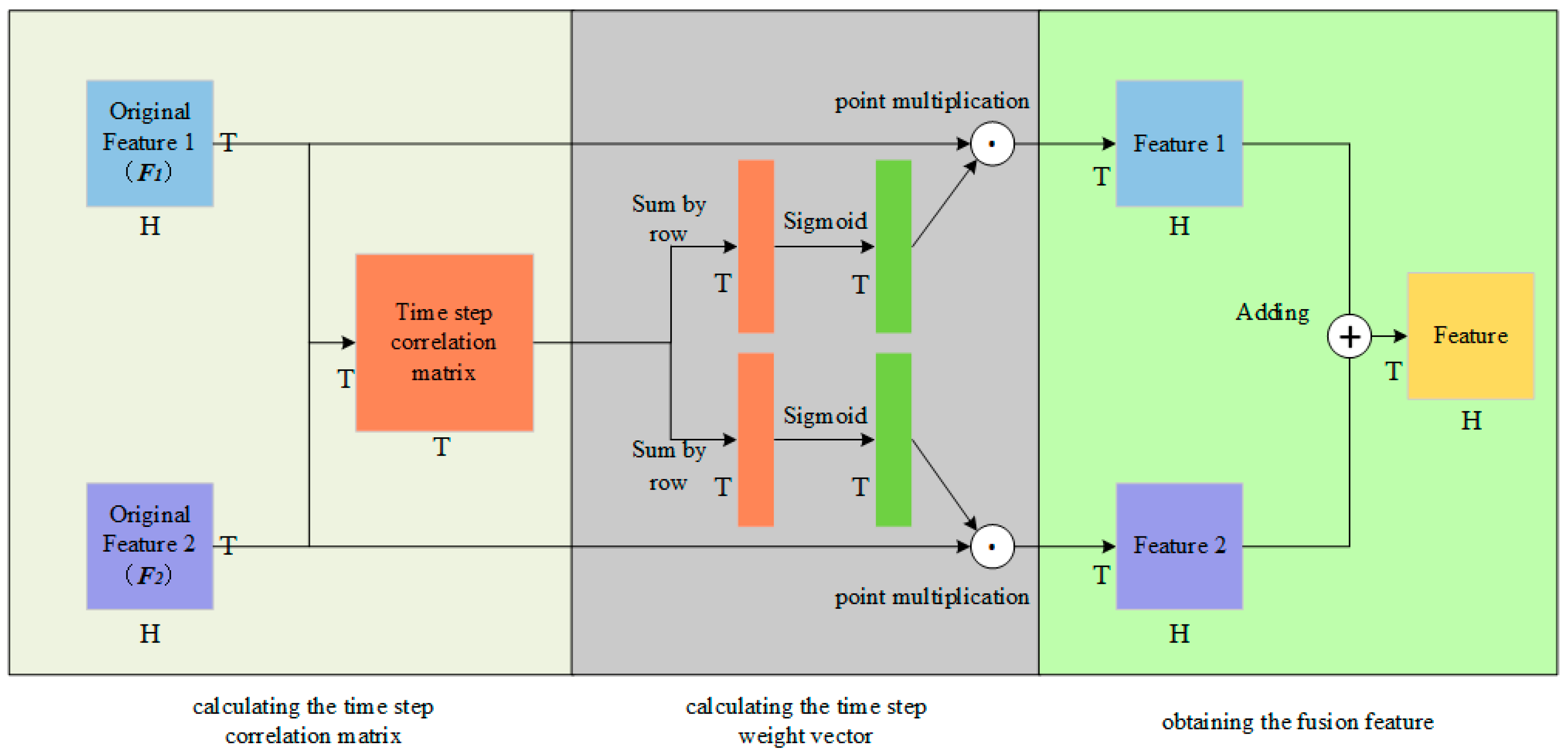
The process of the TCFF module is shown in Figure 6. The method is mainly composed of three parts: calculating the time-step correlation matrix, calculating the time-step weight vector and obtaining the fusion feature. It is assumed that the original features to be fused are F 1 , F 2 H × T , where H and T are the dimensions and time steps of the features. The calculation steps are as follows.
For the two feature vectors F 1 , F 2 H × T of the input module: the correlation of the corresponding time steps is calculated, and two eigenvector covariance matrices TC T × T are obtained. The calculation process is as follows.
F 1 r = F 1 r F ¯ 1 r
where F 1 r represents the r-th time step of feature vector F 1 , F ¯ 1 r represents the matrix consisting of H copies of the mean of feature vector F 1 at the i-th time step, F 1 r , F ¯ 1 r H × 1 . The procedure for calculating the feature vector F 2 is the same as that of F 1 .
The calculation results of each time step F 1 r , F 2 r are spliced to obtain vector F 1 , F 2 H × T . Transpose F 1 and carry out matrix multiplication with F 2 to obtain the time-step correlation matrix.
TC = F 1 T F 2
where denotes matrix multiplication. The time-step correlation matrix TC T × T , T C i j represents the correlation between F 1 the i-th time step and F 2 the j-th time step. The matrix TC allows the statistical correlation between F 1 and F 2 to be analyzed for subsequent more efficient fusion of features.
After the time-step correlation matrix is obtained, the rows and columns are summed, respectively, and two column vectors TC row , TC col T * 1 are obtained, which represent the correlation degree between the i th time step of F 1 and F 2 , and the correlation degree between the j th time step of F 2 and F 1 . According to the magnitude of the summation: the larger the value, the stronger the correlation. For the feature vectors extracted from the same target: the stronger the correlation, the more representative the features are under the current time step, and the features under the current time step should be given a higher weight value. On the contrary, the weaker the correlation, the feature that represents the current time step is not important for the target, and a smaller weight value should be given to avoid information redundancy and to reduce recognition performance. In order to limit the weight value between 0 and 1, we use the Sigmoid function to calculate the two column vectors TC row , TC col , the corresponding weight size. The Sigmoid function is a monotonically increasing function, which can convert the values greater than 0 in the column vector into an interval of 0.5–1 and convert the values less than 0 into 0–0.5. The corresponding weight calculation formula of each feature is as follows:
W F 1 = σ TC row
W F 2 = σ TC col
where σ is the Sigmoid function. The weight vector W F 1 , W F 2 is copied H times and spliced to obtain the new weight vector.
The obtained time step weight vector is multiplied by the corresponding feature vector to obtain the improved feature vector:
F 1 = W F 1 F 1
F 2 = W F 2 F 2
where is the Hadamard product, which represents the multiplication of two matrices in corresponding positions.
Add the obtained feature vectors F 1 , F 2 to obtain the final fusion feature:
F = F 1 + F 2

3. Experimental Results and Analysis

3.1. Introduction to the Dataset

Due to the fact that ship targets are mostly non cooperative targets, it is difficult to establish an HRRP database of targets based on measured ship data. In this paper, we use CAD3D software to build 10 kinds of a 1:1 ship target model and import them into the CST electromagnetic simulation software. The structural parameters of the 10 ship targets are shown in Table 1 [32]. The CST simulation parameters are set as follows: the azimuth angle is 0°~360°, the pitch angle is 90°, and the angle step size is 1°. The center frequency of the radar is 3 GHz, with a bandwidth of 150 MHz. The polarization methods include vertical polarization and horizontal polarization, and the frequency sampling points are 360. The software defaults to the optimal grid analysis size and selects the ray tracing algorithm for the solution. Finally, HRRP data for 360 azimuth angles of 10 types of ship targets are simulated.
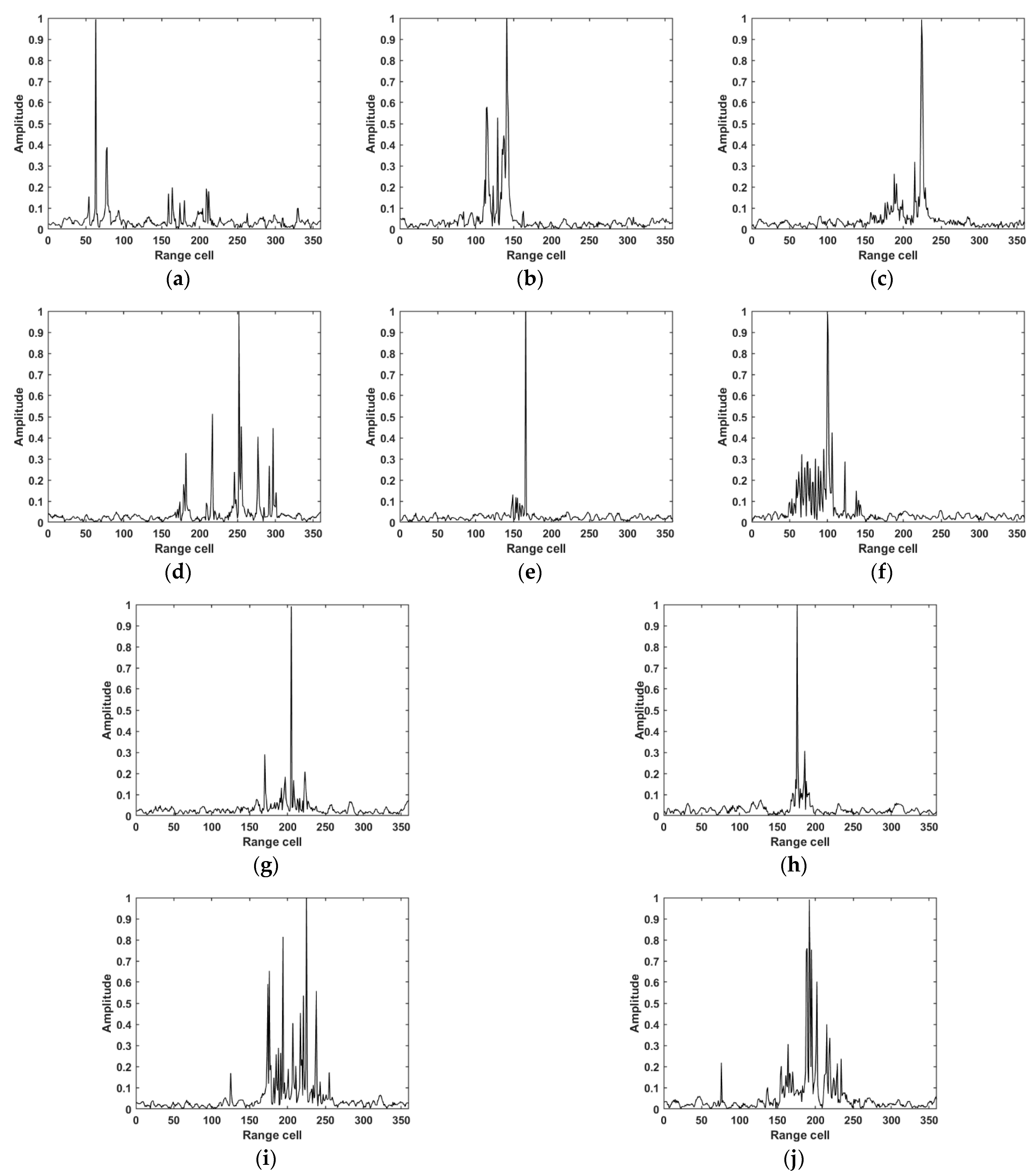
It is well known that the lack of training samples will lead to overfitting of the model. The HRRP data simulated by CST is far from enough and needs to be expanded. In this paper, according to the signal-to-clutter ratio of 10 dB, the original data is expanded by adding clutter that conforms to the K-distribution in three stages. At each signal-to-noise ratio, the data is expanded three times. The HRRP of 10 types of ship targets under the condition of a 10 dB signal-to-noise ratio is shown in Figure 7.
In order to study the improvement effect of recognition performance after HRRP feature fusion in different frequency bands compared with single HRRP recognition performance, 2.85–2.90 GHz, 2.85–2.95 GHz, 2.85–3 GHz, 2.85–3.05 GHz, 2.85–3.10 GHz, 2.90–3.15 GHz, 2.95–3.15 GHz, 3–3.15 GHz, 3.05–3.15 GHz are selected according to the same way as above. The HRRP data set is constructed for 10 types of ship targets in the frequency band of 3.10–3.15 GHz.
In this paper, the model parameters are set as follows: the total number of training epochs is 300, the initial learning rate is 0.03. During the training process, with every 80 iterations, the learning rate decreases to a quarter of the original. The dimensions of hidden layers are set to 128. The optimizer selected the Stochastic Gradient Descent (SGD) method with a batch size of 32. The preprocessed sliding window has a length of d = 48 and a translation distance of l = 24. The number of layers in the feature extraction network is set to 8.

3.2. Recognition Performance

In this section, the recognition performance of each model is tested on ship HRRP data sets of different frequency bands. For the convenience of recording, different frequency bands are numbered, as shown in Table 2. The set of A1–A5 is denoted as A, and the set of B1–B5 is denoted as B.
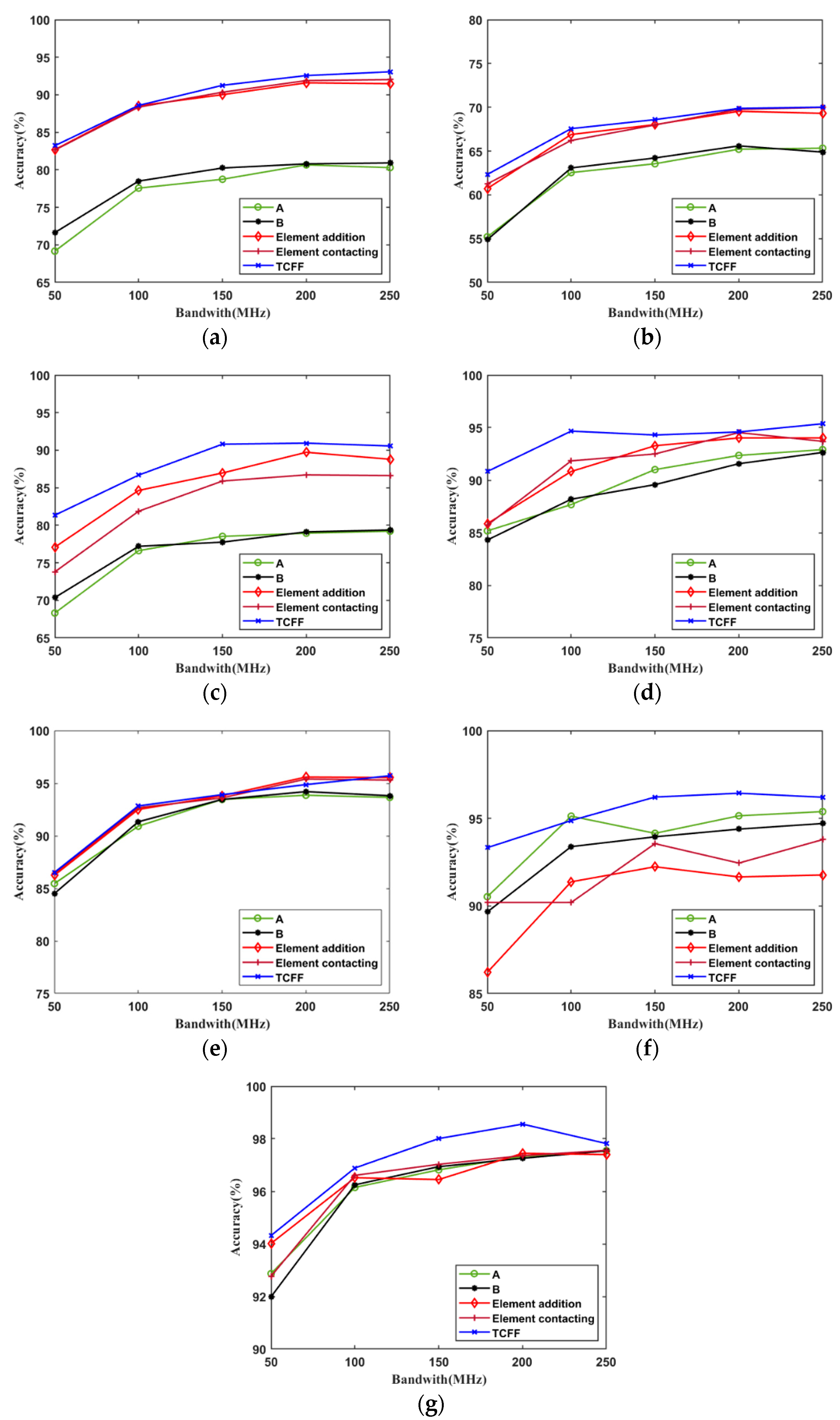
The recognition effects of various models are tested on the HRRP datasets in different frequency bands. At the same time, the HRRPs in different frequency bands under the same bandwidth are fused by TCFF method, and compared with the fusion methods of the element addition and element contacting, respectively. The experimental results are shown in Figure 8a–c 8–14. As shown in Figure 8, the A curve indicates the recognition results using only A1–A5 single data set without fusion processing, where the abscissa 50 MHz corresponds to A1, 100 MHz corresponds to A2, and so on; the marking of the B curve is similar to A. The ‘element addition‘, ‘element contacting‘ and ‘TCFF‘ represent the results of fusion recognition using two datasets. For the ‘element addition‘ curve abscissa, 50 MHz corresponds to the feature fusion of the A1 and B1 datasets, 100 MHz corresponds to the feature fusion of A2 and B2, 150 MHz, 200 MHz, 250 MHz corresponding data sets and so on. The annotation of the curve of the element contacting method and the TCFF method is similar to the element addition method.
Figure 8 records the recognition accuracy of each model in different frequency bands, and the recognition results of the HRRP data feature fusion in different frequency bands with the same bandwidth. It can be seen from the figure that under the condition of a certain signal-to-clutter ratio, in the frequency band of 3–300 MHz bandwidth, the influence of small changes in carrier frequency on recognition performance can be ignored when the bandwidth is the same. Therefore, under the condition of ignoring the influence of carrier frequency, when the bandwidth increases, with the improvement of radar range resolution, the number of scattering points falling into the same range unit decreases, the description of target details by the high resolution range profile is more detailed, and the recognition accuracy is also improved, especially in the range of 50–200 MHz. When the bandwidth increases to 200 MHz, the recognition accuracy is basically stable at an optimal value, and the increase in bandwidth has little effect on the recognition accuracy. On the other hand, the increase in bandwidth leads to the decrease in the length of the range cell, which enhances the detail description of the target HRRP, and it is also more likely to cause the phenomenon of moving across the range cell and destroy the stability of the range profile, which may lead to the decrease in recognition performance.
It can also be found from the figure that by adding an input channel to increase the amount of target information, the feature fusion method of element addition and element contacting can achieve better recognition performance than a single input channel on RNN, LSTM, GRU, SRU and Transformer feature extractors. However, on the R-Transformer and R-DeLighT models, the feature fusion method of element addition and element contacting cannot achieve good results, and even the recognition accuracy is reduced due to the redundancy of irrelevant information. The TCFF feature fusion method proposed in this paper has achieved the best recognition effect on all models and has good generalization and stability. Moreover, compared with the feature fusion method of element addition and element contacting, the TCFF feature fusion method determines the weight of each time step by the correlation strength, and the feature vector obtained by point multiplication with the original feature vector is more separable and achieves better recognition results.
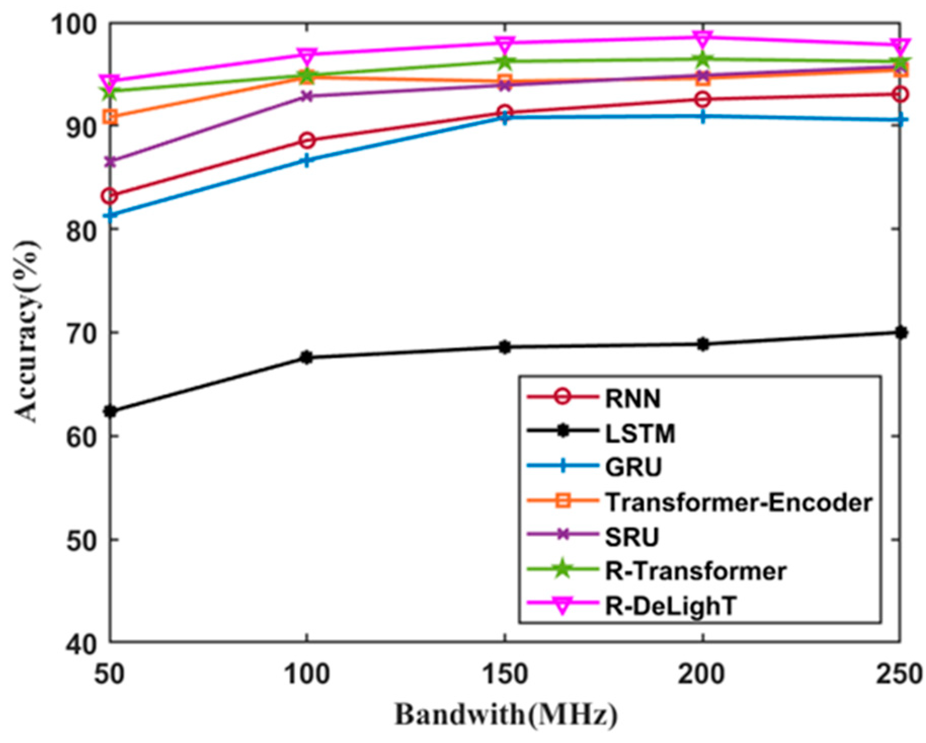
Figure 9 is the recognition result of seven feature extraction models using TCFF fusion method in different frequency bands. It can be seen from the figure that compared with other feature extraction models, the R-DeLighT model is used as the feature extraction model, and combined with the TCFF special fusion method it can achieve the best recognition effect in all frequency bands.

4. Conclusions

Aimed at the fusion problem of multi-source HRRP, this paper proposes a feature fusion method based on time-step correlation. By constructing a dual-channel network model, the two features extracted by the feature extractor are fused according to the time-step correlation. The experimental results on various feature extractors show that the feature fusion method can effectively improve the recognition effect and has good stability.

Author Contributions

Conceptualization, Z.Y. and J.L.; methodology, Z.Y.; software, Z.Y.; validation, L.W. and J.L.; formal analysis, Z.Y.; investigation, Z.Y.; resources, J.L.; data curation, L.W.; writing—original draft preparation, Z.Y.; writing—review and editing, J.L.; visualization, L.W.; supervision, J.L. All authors have read and agreed to the published version of the manuscript.

Funding

This research was funded by the National Natural Science Foundation of China, grant number 61501486.

Informed Consent Statement

Informed consent was obtained from all subjects involved in the study.

Data Availability Statement

Data are available upon reasonable request to the submitting author.

Conflicts of Interest

The authors declare no conflict of interest.

References

  1. Zhang, X.D.; Shi, Y.; Bao, Z. A new feature vector using selected bispectra for signal classification with application in radar target recognition. IEEE Trans. Signal Process. 2001, 49, 1875–1885. [Google Scholar] [CrossRef]
  2. Liao, X.; Runkle, P.; Carin, L. Identification of ground targets from sequential high-range-resolution radar signatures. IEEE Trans. Aerosp. Electron. Syst. 2002, 38, 1230–1242. [Google Scholar] [CrossRef]
  3. Shi, L.; Wang, P.; Liu, H.; Xu, L.; Bao, Z. Radar HRRP statistical recognition with local factor analysis by automatic Bayesian Ying-Yang harmony learning. IEEE Trans. Signal Process. 2010, 59, 610–617. [Google Scholar] [CrossRef]
  4. Du, L.; Wang, P.; Liu, H.; Pan, M.; Chen, F.; Bao, Z. Bayesian spatiotemporal multitask learning for radar HRRP target recognition. IEEE Trans. Signal Process. 2011, 59, 3182–3196. [Google Scholar] [CrossRef]
  5. Zhang, H.; Ding, D.; Fan, Z.; Chen, R. Adaptive neighborhood-preserving discriminant projection method for HRRP-based radar target recognition. IEEE Antennas Wirel. Propag. Lett. 2014, 14, 650–653. [Google Scholar] [CrossRef]
  6. Liu, H.; Feng, B.; Chen, B.; Du, L. Radar high-resolution range profiles target recognition based on stable dictionary learning. IET Radar Sonar Navig. 2016, 10, 228–237. [Google Scholar] [CrossRef]
  7. Zhou, D. Radar target HRRP recognition based on reconstructive and discriminative dictionary learning. Signal Process. 2016, 126, 52–64. [Google Scholar] [CrossRef]
  8. Feng, B.; Chen, B.; Liu, H. Radar HRRP target recognition with deep networks. Pattern Recognit. 2017, 61, 379–393. [Google Scholar] [CrossRef]
  9. Liao, K.; Si, J.; Zhu, F.; He, X. Radar HRRP target recognition based on concatenated deep neural networks. IEEE Access 2018, 6, 29211–29218. [Google Scholar] [CrossRef]
  10. Chen, G.U.O.; Tao, J.I.A.N.; Congan, X.U.; You, H.E.; Shun, S.U.N. Radar HRRP Target Recognition Based on Deep Multi-Scale 1D Convolutional Neural Network. J. Electron. Inf. Technol. 2019, 41, 1302–1309. [Google Scholar]
  11. Du, L.; Liu, H.; Bao, Z.; Xing, M. Radar HRRP target recognition based on higher order spectra. IEEE Trans. Signal Process. 2005, 53, 2359–2368. [Google Scholar]
  12. Du, L.; Liu, H.; Bao, Z.; Zhang, J. Radar automatic target recognition using complex high-resolution range profiles. IET Radar. Sonar. Navig. 2007, 1, 18–26. [Google Scholar] [CrossRef]
  13. Feng, B.; Du, L.; Liu, H.; Fei, L. Radar HRRP target recognition based on K-SVD algorithm. In Proceedings of the 2011 IEEE CIE International Conference on Radar, Chengdu, China, 24–27 October 2011; 1, pp. 642–645. [Google Scholar]
  14. Pan, M.; Du, L.; Wang, P.; Liu, H.; Bao, Z. Multi-task hidden Markov model for radar automatic target recognition. In Proceedings of the 2011 IEEE CIE International Conference on Radar, Chengdu, China, 24–27 October 2011; 1, pp. 650–653. [Google Scholar]
  15. Xu, B.; Chen, B.; Liu, H.; Jin, L. Attention-based recurrent neural network model for radar high-resolution range profile target recognition. J. Electron. Inf. Technol. 2016, 38, 2988–2995. [Google Scholar]
  16. Xu, B.; Chen, B.; Liu, J.; Wang, P.; Liu, H. Radar HRRP target recognition by the bidirectional LSTM model. Xi’an Dianzi Keji Daxue Xuebao J. Xidian Univ. 2019, 46, 29–34. [Google Scholar]
  17. Liu, J.; Chen, B.; Jie, X. Radar high-resolution range profile target recognition based on attention mechanism and bidirectional gated recurrent. J. Radars 2019, 8, 589–597. [Google Scholar]
  18. Jinwei, W.; Bo, C.; Bin, X.; Liu, H.; Jin, L. Convolutional neural networks for radar HRRP target recognition and rejection. EURASIP J. Adv. Signal Process. 2019, 2019, 5. [Google Scholar]
  19. Kuncheva, L.I.; Bezdek, J.C.; Duin, R.P.W. Decision templates for multiple classifier fusion: An experimental comparison. Pattern Recognit. 2001, 34, 299–314. [Google Scholar] [CrossRef]
  20. Liu, Z.G.; Pan, Q.; Dezert, J.; Han, J.; He, Y. Classifier Fusion With Contextual Reliability Evaluation. IEEE Trans. Cybern. 2018, 48, 1605–1618. [Google Scholar] [CrossRef]
  21. Liu, Z.G.; Pan, Q.; Mercier, G.; Dezert, J. A New Incomplete Pattern Classification Method Based on Evidential Reasoning. IEEE Trans. Cybern. 2015, 45, 635–646. [Google Scholar] [CrossRef] [PubMed]
  22. Chen, J. Radar Target Recognition Based on Multi-features Fusion. Bachelor’s Thesis, Xidian University, Xi’an, China, 2010. [Google Scholar]
  23. Li, H.; Qiming, M.; Shuanchuan, D. A feature fusion algorithm based on canonical correlation analysis. Acoust. Electron. Eng. 2015, 20–23. [Google Scholar]
  24. Zhai, J.; Dong, G.; Chen, F.; Xiaodan, X.; Chengming, Q.; Lin, L. A Deep Learning Fusion Recognition Method Based on SAR Image Data. Procedia Comput. Sci. 2019, 147, 533–541. [Google Scholar]
  25. Wu, J.; Zhang, H.; Gao, X. Radar High-Resolution Range Profile Target Recognition by the Dual Parallel Sequence Network Model. Int. J. Antennas Propag. 2021, 2021, 1–9. [Google Scholar] [CrossRef]
  26. Seetharaman, P.; Wichern, G.; Pardo, B.; Roux, J.L. Autoclip: Adaptive gradient clipping for source separation networks. In Proceedings of the 2020 IEEE 30th International Workshop on Machine Learning for Signal Processing (MLSP), Espoo, Finland, 21–24 September 2020; IEEE. pp. 1–6. [Google Scholar]
  27. Xu, B. Radar High Resolution Range Profile Target Recognition based on Temporal Dynamic Methods. Ph.D. Thesis, Xidian University, Xi’an, China, 2019. [Google Scholar]
  28. Hochreiter, S.; Schmidhuber, J. Long short-term memory. Neural Comput. 1997, 9, 1735–1780. [Google Scholar] [CrossRef]
  29. Cho, K.; van Merriënboer, B.; Gulcehre, C.; Bahdanau, D.; Bougares, F.; Schwenk, H.; Bengio, Y. Learning phrase representations using RNN encoder-decoder for statistical machine translation. arXiv 2014, arXiv:1406.1078. [Google Scholar]
  30. Lei, T. Fast Neural Network Implementations by Increasing Parallelism of Cell Computations. U.S. Patent 11,106,975, 31 August 2021. [Google Scholar]
  31. Vaswani, A.; Shazeer, N.; Parmar, N.; Uszkoreit, J.; Jones, L.; Gomez, A.N.; Kaiser, Ł.; Polosukhin, I. Attention is all you need. Adv. Neural Inf. Process. Syst. 2017, 8, 5598–6008. [Google Scholar]
  32. Yue, Z.; Lu, J.; Wan, L. Lightweight Transformer Network for Ship HRRP Target Recognition. Appl. Sci. 2022, 12, 9728. [Google Scholar] [CrossRef]
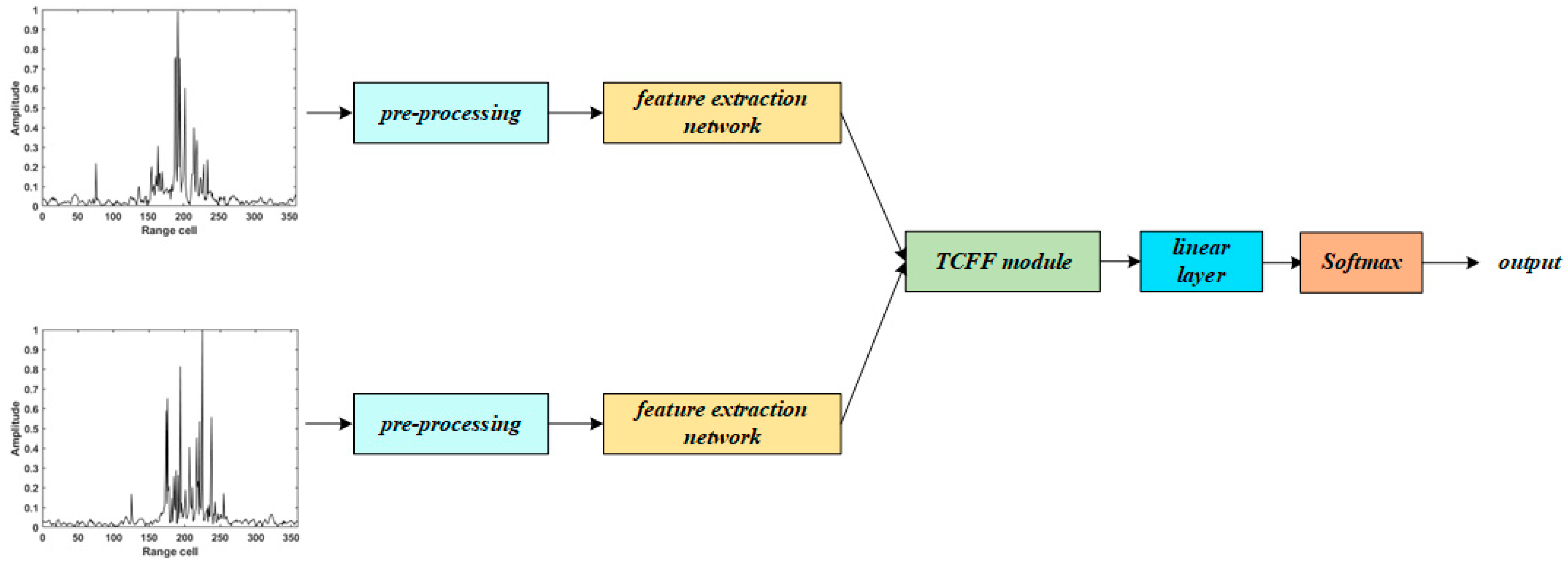
Figure 1. HRRP recognition model integrated into the TCFF module.
Applsci 13 05286 g001
Figure 2. Structure diagram of the R-DeLighT model.
Applsci 13 05286 g002
Figure 3. Structure diagram of the local RNN module with sliding window size of 3.
Applsci 13 05286 g003
Figure 4. Comparison of the standard Transformer model encoder structure (left) and the Transformer model encoder structure combined with GLTs (right).
Applsci 13 05286 g004
Figure 5. Characteristic mixing process in dimension-up phase of GLTs module.
Applsci 13 05286 g005
Figure 6. Flow chart of TCFF module.
Applsci 13 05286 g006
Figure 7. HRRP of class 10 ship targets. (aj) represent ships 1–10.
Applsci 13 05286 g007
Figure 8. The recognition accuracy of different model in different frequency bands and the recognition accuracy after feature fusion. (ag) indicates the LSTM, RNN, GRU, Transformer–Encoder, SRU, SRU–Transformer, R–DeLighT model.
Applsci 13 05286 g008
Figure 9. The accuracy of TCFF feature fusion recognition in different frequency bands of seven feature extraction models.
Applsci 13 05286 g009
Table 1. Structural parameters of 10 types of ship targets.
Ship NumberLength (m)Width (m)
1182.824.1
2153.820.4
3162.921.4
499.615.2
5332.876.4
6337.277.2
717.13.6
8143.415.2
917.64.5
1016.34.7
Table 2. Corresponding numbers of ship target HRRP data sets in different frequency bands.
NumberOperational Frequency Band (GHz)Bandwidth (MHz)
A12.85–2.9050
A22.85–2.95100
A32.85–3.00150
A42.85–3.05200
A52.85–3.10250
B13.10–3.1550
B23.05–3.15100
B33.00–3.15150
B42.95–3.15200
B52.90–3.15250
Disclaimer/Publisher’s Note: The statements, opinions and data contained in all publications are solely those of the individual author(s) and contributor(s) and not of MDPI and/or the editor(s). MDPI and/or the editor(s) disclaim responsibility for any injury to people or property resulting from any ideas, methods, instructions or products referred to in the content.