Abstract
Traditional land-use systems can be modified under the conditions of climate change. Higher air temperatures and loss of productive soil moisture lead to reduced crop yields. Irrigation is a possible solution to these problems. However, intense irrigation may have contributed to land degradation. This research assessed the ameliorative potential of soil and produced large-scale digital maps of soil properties for arable plot planning for the construction and operation of irrigation systems. Our research was carried out in the southern forest–steppe zone (Southern Ural, Russia). The soil cover of the site is represented by agrochernozem soils (Luvic Chernozem). We examined the morphological, physicochemical and agrochemical properties of the soil, as well as its heavy metal contents. The random forest (RF) non-linear approach was used to estimate the spatial distribution of the properties and produce maps. We found that soils were characterized by high organic carbon content (SOC) and neutral acidity and were well supplied with nitrogen and potassium concentrations. The agrochernozem was characterized by favorable water–physical properties and showed good values for water infiltration and moisture categories. The contents of heavy metals (lead, cadmium, mercury, cobalt, zinc and copper) did not exceed permissible levels. The soil quality rating interpretation confirms that these soils have high potential fertility and are convenient for irrigation activities. The spatial distribution of soil properties according to the generated maps were not homogeneous. The results showed that remote sensing covariates were the most critical variables in explaining soil properties variability. Our findings may be useful for developing reclamation strategies for similar soils that can restore soil health and improve crop productivity.
1. Introduction
Research on the Earth’s climate change indicates a warming trend [1,2]. Predictive modelling of future temperature change shows further climate warming due to intensive human-made impacts [3]. Climate change is transforming native ecosystems [4], including agricultural systems, which are exceptionally important in the context of the increasing population of the Earth to provide sufficient food of good quality [5].
As the climate warms, the frequency, duration and intensity of droughts are expected to increase. Such conditions will significantly limit crop production options and reduce crop yields [6,7]. For example, rice yields in China [8] and Korea [9], cotton and sorghum in South Africa [10] and olives in Portugal [11] are threatened.
This raises the need for climate-smart agriculture [12]. Irrigation is one such effective method [13]. Soil irrigation is essential for ensuring the healthy growth of crops and plants. Irrigation helps to supply water to the root zone of plants, which is critical for their survival and growth. Moreover, complementary irrigation is critical to ensuring crop yields and agricultural quality in many regions of the Earth [14,15]. Under these conditions, irrigation is ranked first among other aspects of soil formation, as its intensification leads to changes in the physical [16], water [17], physicochemical [18,19], chemical [20,21] and biological [22,23] soil regimes. Thus, irrigation is an influential factor in transforming and transferring matter and energy in a soil profile.
The main requirements for reclamation and irrigation measures are assessing soil conditions and creating large-scale up-to-date maps. The latter requirement is necessary to study and understand the spatial distribution of soil nutrients. The use of machine learning techniques in digital soil mapping is now being actively implemented [24]. One of the most popular methods is the random forest (RF) classification algorithm, which consists of many decision trees [25]. This algorithm has demonstrated reliable results for digital mapping of soil properties at different scales [26,27,28]. For example, Wiesmeier et al. [29] applied the RF approach for the spatial prediction of soil organic carbon (SOC) stocks in Inner Mongolia, Northern China. The authors showed that land use, soils and geology were the most important variables influencing SOC storage. Similarly, this method was applied to digital mapping of SOC and calcium carbonate equivalent contents, where it was found that the key factors for the distribution of properties were remote sensing data [30].
In the context of climate change, proper soil irrigation is even more critical as it can help to mitigate the impacts of drought and extreme weather events, which are becoming more frequent and severe due to climate change. Efficient use of water through soil irrigation can help to conserve water resources, reduce greenhouse gas emissions associated with water pumping and transportation and enhance soil carbon sequestration, which can help to mitigate climate change. Climate change equally occurs in forest–steppe zones, including in the study region [31,32]. Such conditions make it necessary to increase the share of irrigated land and design new irrigation systems. Hence, detailed land cover studies and mapping are needed in planning irrigation system construction and operations to avoid degradation processes (water and wind erosion, accumulation of toxic salts, erosion of soil structure and loss of SOC and nutrients). The study’s primary purpose is to assess the soils for use in irrigated agriculture in the forest–steppe zone of the Republic of Bashkortostan (Russia). Therefore, the objectives of this study are the following: (i) study the physicochemical properties of soils, (ii) assess the geochemical condition of soils, and (iii) conduct the digital mapping of soil properties using the RF approach in combination with remote sensing and topography data.
2. Materials and Methods
2.1. Site Description
The study site (327 hectares) is an arable plot located in the southern forest–steppe zone, on the Belaya River’s second floodplain terrace (Figure 1). The study area is characterized by flat terrain and is located near the river, which made it suitable for involvement in arable farming and further irrigation. The soil cover of the site is represented predominantly by agrochernozem soils (Luvic Chernozem). There are also small areas of meadow–swamp soils. Meadow–swamp soils are formed in drainless declines and karst craters. When the meltwater and the soil–ground water close to the surface are stagnant, with gleying processes developing. These soils are not plowed because they are unsuitable for agricultural use. For these reasons, no more specific study of meadow–swamp soils has been conducted.
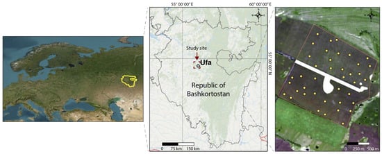
Figure 1.
Location of the study site and distribution of samples (image source: Sentinel-2A—natural color composite).
The climate of the study area is described as continental and moderately arid. The average annual air temperature is 2.8 °C, the mean January temperature is −15 °C and the absolute minimum is −46 °C. The mean July temperature is +19 °C, and the absolute maximum is +38 °C. Droughts are frequent in spring, autumn and the second half of the summer.
The terrain of the study area is generally levelled; the gradients are small, with a slope predominance of 1–2° (0–1° = 112 ha (34.2%); 1–2° = 172 ha (52.6%); 2–4° = 42 ha (12.8%); 4–6° = 1 ha (0.4%)), but there are karst funnels. The height above sea level varies from 80 to 90 m. Groundwater is found at a depth of 8 m; water composition is hydrocarbon–calcium–magnesium with a 0.3 g/L. Water for irrigation would be taken from the Belaya River. The water composition is hydrocarbon–calcium with mineralization of 0.3–0.6 g/L.
2.2. Data Collection and Chemical Analysis
For this study, we excavated 15 full-length sections on the site. Soil samples were collected from each established genetic horizon over the entire width of the soil profile [33]. Additionally, 40 soils were sampled from the upper horizon (0–10 cm) to assess the spatial distribution of soil properties. The selected samples were air-dried, ground and carefully passed through a 1 mm sieve. Soil descriptions in the field and further agrochemical analyses were carried out using conventional methods [34,35,36]. Under laboratory conditions, SOC content, soil acidity (pH), soluble salts, alkaline hydrolyzed nitrogen (N), available phosphorus (P2O5) and potassium (K2O), exchangeable calcium (Ca2+) and magnesium (Mg2+) cations and exchangeable sodium (Na+) were determined.
The water–physical properties of soils were measured according to Shein and Karpachevskii guidelines [37]. The heavy metal content was determined in conformity with the methodological guidelines [38]. Soil availability criteria for organic matter, nutrients and micronutrients were assessed by Kiryushin [39]. The index of soil quality and yield was defined by Karmanov et al. [40].
Soil categorization and the characteristics of the ground profile and layers were accomplished considering substantive genetic classification [41]. The World Reference Base duplicated the consequent soil type name for Soil Resources [42].
2.3. Random Forest
We applied the RF algorithm for the spatial prediction of soil properties because it is the most popular in digital soil mapping studies [43]. Moreover, this method is superior to other machine learning methods, as shown in a variety of studies [28,44,45,46,47]. RF is an ensemble learning method for classification and regression tasks. In a model, each decision tree in the forest is built using a random subset of the input data and a random subset of the input features. Then, the results of all individual trees are aggregated to make a single prediction. We defined the default parameters required by the RF model: the number of trees to be built in the forest (ntree) and the number of predictors to be used in each tree-building process (mtry). We set the parameters as follows: ntree = 500 and mtry = 4.
The recursive feature elimination (RFE) method was applied to select an optimal set of environmental auxiliary variables among all covariates [48]. The algorithm works by backward selection, where the least promising predictors are excluded from the model based on an initial predictor importance measure.
2.4. Environmental Variables
The environmental covariates used for digital mapping included Sentinel-2A satellite data (S2A) and topographic attributes. S2A data were selected during the period with minimal vegetation (bare soil). The dataset of 25 May 2019, which was used for study, matched these parameters. Satellite bands and the Normalized Difference Vegetation Index (NDVI) were used. Relief attributes were calculated using a 30 m resolution digital relief model (NASA’s Shuttle Radar Topography Mission (SRTM), https://www2.jpl.nasa.gov/srtm (accessed on 20 January 2023)). The topographical attributes included elevation, aspect, slope, multiresolution of ridge top flatness (MrRTF) and (MrVBF) multiresolution valley bottom flatness indices. The environmental variables used for modelling are presented in Table 1.

Table 1.
Environmental covariates used for digital mapping.
2.5. Validation and Statistical Analyses
A leave-one-out cross-validation (LOOCV) approach was applied to evaluate the prediction performance of RF models. LOOCV cross-validation is appropriate for a small dataset and consists of using all training data leaving one out. The accuracy of the predictive model was estimated using a mean error (ME) and a root-mean-square error (RMSE) (Equations (1) and (2)):
where Oi and Pi are observed and predicted values of soil properties, respectively, and n is the number of samples.
Statistical data processing, digital mapping and model accuracy assessment were performed in R and RStudio.
3. Results
The agrochernozem soils under study formed on well-watered sections on carbonate eluvial–diluvial clays and heavy loams. The morphological structure characteristics of those soil profiles were that the A1 humus-accumulative horizon was an average of ≈84 cm, and the medium depth of a layer A1 + ABca holds ≈125 cm. Horizon A was divided into the upper plowable part (Aplow) with a thickness of ≈28 cm and the plough-pan part (A1). We described the soil section on the flat area (Table 2).
Table 2.
Description of soil horizon.
The morphological description of the soil profile showed that the humus-accumulative horizon (A) was characterized by a dark grey or almost black color. The texture of the Aplow, A1 and A1Bca horizons was classified as heavy loamy. There were many roots at the toplayer. The top plowable part’s structure was powdery–lumpy, the A1 plough-pan part was granular and the A1Bca horizon became coarse-grained. The upper bound for detecting carbonates as a mycelium occurred inside the A1Bca horizon. The Bca horizon was characterized by a lumpy structure that becamelarge-cloddy within the Cca layer.
The analysis of soil chemical properties is presented in Table 3. The soils were characterized by a neutral reaction in the upper horizons (pH H2O 6.6–6.9), but with depth, the reaction varies to weakly alkaline (pH H2O 8.3). The average SOC content was 4.4% in the plowable horizon and decreased by 3.7% in A1 and 0.6% in the C layer. The content of hydrolyzable nitrogen ranged from 186 to 26 mg/kg (from Aplow to Cca layer) and exchangeable potassium from 152 to 54 mg/kg, which, in the studied soils, was classified as “high” according to grading [41]. However, the values of available phosphorus were insignificant (51–17 mg/kg). The values of Ca2+ (34.7–27.3 mg/kg) and Mg2+ (7.7–5.4 mg/kg) varied approximately in the same ranges across all horizons. The base saturation values ranged from 98% in the top layer to 100% in the Cca horizon, while the range of solids values ranged from 0.05 to 0.02% and also tended to decrease with depth.
Table 3.
Description of soil horizon 1.
Conducive aquatic and physical properties are crucial indicators of the suitability of soils for irrigated agriculture [49,50]. These properties influence soil water, air and nutrient status, crop yields and agricultural product quality [51,52]. The bulk density of the humus-accumulative horizon of the investigated soils was optimal for most crops (1.02 g/cm3 in the to player and 1.44 g/cm3 in Cca) (Table 4). Simultaneously, with depth, the density gradually increases, an illuvial horizon was compacted (1.39 g/cm3), and a soil-forming rock was dense (1.44 g/cm3).
Table 4.
Water–physical properties of the agrochernozem soils 1.
The hardness of the soil lumps also increased with depth. With the optimal soil texture, humus-accumulative horizons possess a significant rate of air space porosity. The water capacity in the plowable layer was equal to 43.0% (field moisture capacity), 45.0% (capillary moisture capacity) and 53.7% (total moisture capacity). With depth, these values decreased to 23.9, 25.9 and 29.3% in the Cca horizon, respectively. The wilting point of the A1 humus-accumulative horizon was 14.2–14.3% and decreased to 11.8% with depth. The content of silt (56.2–65.9%) was dominant in the composition of all soil horizons; then, clay and sand contents were descending (21.4–28.9 and 7.8–14.9, respectively).
Figure 2 shows water infiltration of the agrochernozem. Determining water infiltration showed that the average speed of water absorption from the soil surface was 1.52 mm/min and from a depth of 50 cm—2.41 mm/min, which, according to the classification of Kachinsky [37], belongs to the medium and high categories of water infiltration, respectively.
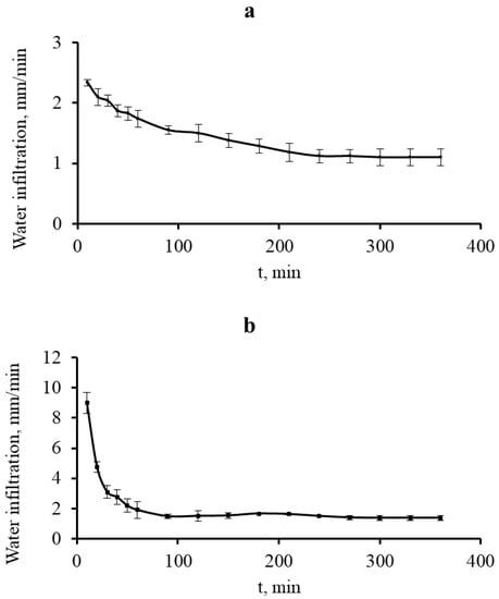
Figure 2.
Water infiltration of the agrochernozem studied: (a) water absorption speed from the soil surface; (b) water absorption speed from a depth of 50 cm.
Land irrigation increases the likelihood of contamination of soils and agricultural products by various pollutants, including heavy metals [53,54]. Toxicants may also become more mobile in the soil profile [55]. The analysis of micronutrients and heavy metals showed low and medium cobalt, zinc and copper contents (Table 5). The average values of the heavy metals and micronutrient contents were 2.71 mg/kg for Pb, 0.18 mg/kg for Cd, 0.024 mg/kg for Hg, 0.13 mg/kg for Co, 0.33 mg/kg for Zn, 0.11 mg/kg for Cu and 11.27 mg/kg for Mn at the Aplow layer. The Pb, Cd and Hg contents were well below the maximum allowable concentrations. It can be assumed that if there were no pollutants in the water used for irrigation, there will be no risk of contamination from agricultural produce.
Table 5.
Heavy metals and micronutrient content 1.
The effectiveness of soil element prediction models using the RF approach according to the error metrics (ME and RMSE) is presented in Table 6. As an indicator of site fertility, the SOC prediction model showed the RMSE value of 0.60, comparable to that of other authors [56,57]. The RMSE values for pH, Mg, Ca, N, P and K were 0.48, 1.56, 2.51, 2.92, 1.57 and 4.57, respectively.
Table 6.
Test performance of the RF for soil properties at 0–10 cm depth.
The top three important variables for each soil feature were different. The most important variables to explain the spatial distribution of SOC, Ca, N, P and K contents were remote sensing data, while the terrain covariates were responsible for pH and Mg prediction. For example, S2A B12 band, NDVI and aspect were responsible for the SOC variation. Since there was a close positive correlation between the SOC content and N (r = 0.86), the key predictors of these parameters were practically the same. Terrain attributes were less responsible for agrochemical property variations, which can be explained by the relatively flat topography of the plots, low pedologic diversity and insufficient spatial resolution of the DEM. The variation in pH levels was entirely controlled by the slope, aspect and elevation covariates. The slope variable was also the leading predictor of Mg content. The spatial distribution of the remaining elements was controlled by both types of variables.
The generated digital maps of soil properties in the upper horizon (0–10 cm) using the RF method are shown in Figure 3. The spatial distribution of the elements was not homogeneous. The elevated concentrations of pH, Ca, P and K were found mainly in the northern part, while Mg content was found in the southern part of the plot.
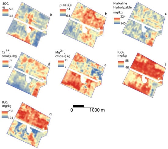
Figure 3.
The spatial distribution of soil agrochemical properties using the random forest method. Areas with vegetation are masked by white color. SOC (a); pH (b); N (c); Ca (d); Mg (e); P (f); and K (g).
4. Discussion
The assessment and digital mapping of soil properties for reclamation measurements is a complex process that requires careful planning and implementation. By using a combination of soil analysis, spatial mapping, modelling and monitoring, it is possible to identify the factors that contribute to soil degradation and develop effective reclamation strategies to improve soil health and productivity.
The chemical and water–physical properties of the studied agrochernozem soils correspond to analogues in this region. For example, the granulometric composition was also classified as heavy loam in horizons Aplow, A1, AB and B, while the wilting point values ranged from 12.7% in the plough horizon to 10.6% in the lower one [58]. The pH and SOC values were also comparable with our results. However, the concentrations of P2O5 and K2O in the arable horizon were higher, which is probably due to the application of fertilizers. According to Figure 2, in the upper layer, the rate of water absorption was gradual due to heavy loamy texture and high SOC content. The lower horizons (>50 cm) were clayey, compacted, without structural aggregates and accordingly flow poorly. A sharp spike in water absorption in the lower horizon is associated with the fractured structure of the soil profile and karst. However, the absorption of water stops due to the clay structure. Therefore, it is necessary to set watering rates for irrigation.
Long-term irrigation risk salinization of soils and alteration of cation composition [55,58], resulting in increased toxicity and structural breakdown. In our study, soils were saturated with calcium-dominated bases. Exchangeable sodium in absorbed cations was not detected. This soil is highly resistant to anthropogenic effects [39]. For example, earlier, it was shown that despite the deterioration of the properties of arable chernozem as a result of prolonged conventional plowing, they remain more resistant to degradation compared to other soils [59]. The water-soluble salt content in the profile is relatively low, and the soil is characterized as not saline. It is likely that hydrocarbon–calcium water and irrigation regimes do not pose a threat to soil salinization. However, the irrigation process and soil condition should be monitored. Previously, the effect of long-term irrigation on the properties of Luvic Chernozem in this region has been shown [60]. It was found that agrophysical, chemical and physicochemical properties of the soil deteriorated, and salt content increased over a 30-year period of irrigation.
The content of heavy metals did not exceed the maximum permissible concentrations, which was comparable with other studies in this region. For instance, average values of Pb, Cd and Zn were 5.1, 0.28 and 1.48, respectively, in the arable layer of chernozem, although the Mn values were half as much [61].
As an integral indicator of ground properties [62], a soil quality rating based on criteria such as humus-accumulative capacity, acidity, SOC content and mobile phosphorus showed that the soil quality index was 74 points, with a maximum of 100 points for the reference soil (Calcic Chernozem). Given the crop, the soil quality index was 62 for wheat production and 65 for sunflower grain production. Here, the decrease in the quality index was due to a deficit of productive soil moisture.
Lamichhane et al. [46] after analyzing 120 studies concluded that vegetation indices were found to be more influential in predicting SOC in small plots. At the same time, we hypothesize that soil spectral reflectance explains a key influence on the SOC prediction, as darker color corresponds to increased organic carbon, and therefore N, compared to paler color [63]. Thus, numerous studies have shown good results for spatial prediction of soil properties on arable land using remote sensing data [64,65]. However, Suleymanov et al. [66] applied a Support Vector Machine method in combination with terrain attributes for modeling soil properties on arable chernozem. The authors achieved RMSE coefficients of 5.33 for Ca, 0.73 for P and 32.34 for K. In another study on the digital mapping of agrochernozems properties, the authors reached RMSE values of 4.4, 27.5 and 14.6 for nitrogen, phosphorus and potassium, respectively, using machine learning methods in combination with remote sensing data and collocated soil parameters maps [67]. Thus, Tziachris et al. [68] previously showed that the measured collocated soil parameters that were used as covariates (clay, electric conductivity and pH) had more influence for predicting soil organic matter than the environmental parameters due to flat terrain. In another research, it was reported that the key variables for explaining the spatial patterns of SOC concentration were a clay map, remote sensing data and distance from the river [69]. Similarly, Were et al. [70] showed that a total nitrogen map was the most important variable for the spatial assessment of SOC stocks. Thus, different maps of various soil parameters can be useful information for spatial prediction at different depths in future studies.
External influences on soils directly affect qualitative and quantitative indicators, as well as their spatial variability. Since irrigation directly affects soil cover and its properties, we assume that the spatial distribution of properties will also be subject to change. For example, Biswas and Mojid [71] showed that SOC, total nitrogen and phosphorus concentrations increased significantly as a result of wastewater irrigation in the topsoil layer. The study conducted on three forage farms irrigated for more than 30 years in Saudi Arabia showed that most soil properties were characterized by moderate or strong spatial dependence [72]. At the same time, changes in soil variability can also be accompanied by fertilization, erosion, plot divisions, crop rotations and change or alternation of tillage practices [73,74]. Thus, permanent irrigation can affect the content and spatial variability of soil parameters, which requires more frequent digital mapping.
Further work to improve the predictive accuracy can be achieved by applying additional variables to explain the variation in properties, unmanned aerial vehicles (UAV) [75,76], predictive techniques that take into account spatial dependence [77] and collecting more soil samples. For example, remote sensing data, such as S2A, has a spatial resolution of 10 m, which may not be sufficient for the digital mapping of soil properties in small areas. Specifically, Baltensweiler et al. [27] concluded that microtopography has the most significant impact on soil acidity variability. Moreover, UAV provides more flexibility in the frequency of the survey and minimizes the effects of weather conditions such as cloud cover [78]. Nevertheless, the main limitation of UAV is the spatial coverage, which makes it difficult to map soil properties at the regional level. Nevertheless, the application of UAV seems to be a more rational solution for assessing the spatial distribution of soil properties on irrigated lands.
5. Conclusions
Global climate change is occurring on all parts of the Earth and is accompanied by an increase in the frequency of natural disasters. The trend of increasing average annual temperatures and decreasing precipitation creates a dangerous and unstable situation for agriculture. In this regard, irrigation will be expanded and actively applied, which will certainly affect the qualitative and quantitative characteristics of soils. Therefore, such fertile soils and the dynamics of their change under the influence of irrigation should be examined and studied.
In this study, we examined the soil cover of the arable plot designated for irrigation in the southern forest–steppe zone of Russia (Southern Ural). The evaluation of morphological, physicochemical and agrochemical properties of soils showed that they had a thick humus-accumulative horizon, and were characterized by high organic carbon content (SOC) and neutral acidity. These soils were well supplied with nitrogen and potassium concentrations, but available phosphorus levels were low.
The agrochernozem was characterized by favorable water–physical propertiesand showed good values for water infiltration and moisture categories. The granulometric composition of the soil horizons (Aplow–Bca) was characterized as heavy loamy, while Cca layer was classified as heavy clay. These soils have high potential fertility and are favorable for improving irrigation.
These arable soils did not contain heavy metals or water-soluble salts at concentrations harmful to plants. The availability of micronutrients (lead, cadmium, mercury, cobalt, zinc and copper) was low, whereas manganese content was moderate.
Using the random forest machine learning method, we modelled the spatial distribution and produced digital maps of the soil elements. In general, remote sensing variables were the most effective covariates in predicting soil parameters, which is explained by the spectral reflectance of bare soil. However, relief attributes can also explain the variation of soil properties on heterogeneous terrain and with higher spatial resolution. Thus, significant improvement in the spatial assessment of soil properties can be achieved using unmanned aerial vehicles and a good number of soil samples.
Overall, the assessment and spatial modeling of agrochernozem properties are necessary to monitor the effectiveness of reclamation measures. By tracking changes in soil properties over time, we can determine whether our reclamation efforts are having the desired impact and make adjustments as necessary.
Author Contributions
Conceptualization, R.S. (Ruslan Suleymanov) and E.A.; methodology, A.S.; software, A.S.; validation, I.A. and G.G.; formal analysis, I.A.; investigation, R.S. (Ruslan Suleymanov), A.S., G.Z., E.A., I.A. and G.G.; resources, R.S. (Ruslan Suleymanov); data curation, E.A.; writing—original draft preparation, R.S. (Ruslan Suleymanov) and G.Z.; writing—review and editing, R.S. (Ruslan Shagaliev), E.A., A.S. and G.Z.; visualization, G.G.; supervision, R.S. (Ruslan Shagaliev) and E.A.; project administration, R.S. (Ruslan Shagaliev) and E.A.; funding acquisition, R.S. (Ruslan Suleymanov), G.Z. and R.S. (Ruslan Shagaliev). All authors have read and agreed to the published version of the manuscript.
Funding
This study was funded by the Ministry of Science and Higher Education of the Russian Federation «PRIORITY 2030» (National Project «Science and University»).
Institutional Review Board Statement
Not applicable.
Informed Consent Statement
Not applicable.
Data Availability Statement
Data are available upon request.
Conflicts of Interest
The authors declare no conflict of interest.
References
- Thorne, P. Global surface temperatures. In Climate Change: Observed Impacts on Planet Earth, 2nd ed.; Letcher, T.M., Ed.; Elsevier: Amsterdam, The Netherlands, 2016; pp. 21–35. [Google Scholar]
- Zalasiewicz, J.; Williams, M. Climate change through Earth’s history. In Climate Change: Observed Impacts on Planet Earth, 2nd ed.; Letcher, T.M., Ed.; Elsevier: Amsterdam, The Netherlands, 2016; pp. 3–17. [Google Scholar]
- Abiodun, B.J.; Adedoyin, A. A modelling perspective of future climate change. In Climate Change: Observed Impacts on Planet Earth, 2nd ed.; Letcher, T.M., Ed.; Elsevier: Amsterdam, The Netherlands, 2016; pp. 355–371. [Google Scholar]
- Hannah, L. Ecosystem change. In Climate Change Biology; Hannah, L., Ed.; Academic Press: London, UK, 2011; pp. 101–130. [Google Scholar]
- Dixon, G.R. The impact of climate and global change on crop production. In Climate Change; Letcher, T.M., Ed.; Elsevier: Amsterdam, The Netherlands, 2009; pp. 307–324. [Google Scholar]
- Ronco, P.; Zennaro, F.; Torresan, S.; Critto, A.; Santini, M.; Trabucco, A.; Zollo, A.L.; Galluccio, G.; Marcomini, A. A risk assessment framework for irrigated agriculture under climate change. Adv. Water Resour. 2017, 110, 562–578. [Google Scholar] [CrossRef]
- Bigelow, D.P.; Zhang, H. Supplemental irrigation water rights and climate change adaptation. Ecol. Econ. 2018, 154, 156–167. [Google Scholar] [CrossRef]
- Ding, Y.; Wang, W.; Zhuang, Q.; Luo, Y. Adaptation of paddy rice in China to climate change: The effects of shifting sowing date on yield and irrigation water requirement. Agric. Water Manag. 2020, 228, 105890. [Google Scholar] [CrossRef]
- Lee, S.H.; Choi, J.Y.; Hur, S.O.; Taniguchi, M.; Masuhara, N.; Kim, K.S.; Hyun, S.; Choi, E.; Sung, J.H.; Yoo, S.H. Food-centric interlinkages in agricultural food-energy-water nexus under climate change and irrigation management. Resour. Conserv. Recycl. 2020, 163, 105099. [Google Scholar]
- Shamseddin, M.A. Impacts of drought, food security policy and climate change on performance of irrigation schemes in Sub-saharan Africa: The case of Sudan. Agric. Water Manag. 2020, 232, 106064. [Google Scholar]
- Fraga, H.; Pinto, J.G.; Santos, J.A. Olive tree irrigation as a climate change adaptation measure in Alentejo, Portugal. Agric. Water Manag. 2020, 237, 106193. [Google Scholar] [CrossRef]
- Lal, R. Climate change and agriculture. In Climate Change: Observed Impacts on Planet Earth, 2nd ed.; Letcher, T.M., Ed.; Elsevier: Amsterdam, The Netherlands, 2016; pp. 465–489. [Google Scholar]
- Malek, K.; Adam, J.C.; Stöckle, C.O.; Peters, R.T. Climate change reduces water availability for agriculture by decreasing non-evaporative irrigation losses. J. Hydrol. 2018, 561, 444–460. [Google Scholar] [CrossRef]
- Cody, K.C. Upstream with a shovel or downstream with a water right? Irrigation in a changing climate. Environ. Sci. Policy 2018, 80, 62–73. [Google Scholar] [CrossRef]
- Rio, M.; Rey, D.; Prudhomme, C.; Holman, I.P. Evaluation of changing surface water abstraction reliability for supplemental irrigation under climate change. Agric. Water Manag. 2018, 206, 200–208. [Google Scholar] [CrossRef]
- Drewry, J.J.; Sam Carrick, S.; Penny, V.; Houlbrooke, D.J.; Laurenson, S.; Mesman, N.L. Effects of irrigation on soil physical properties in predominantly pastoral farming systems: A review. N. Zeal. J. Agric. Res. 2021, 64, 483–507. [Google Scholar] [CrossRef]
- Wang, X.; Wang, H.; Si, Z.; Gao, Y.; Duan, A. Modelling responses of cotton growth and yield to pre-planting soil moisture with the CROPGRO-Cotton model for a mulched drip irrigation system in the Tarim Basin. Agric. Water Manag. 2020, 241, 106378. [Google Scholar] [CrossRef]
- Abegunrin, T.P.; Awe, G.O.; Idowu, D.O.; Adejumobi, M.A. Impact of wastewater irrigation on soil physico-chemical properties, growth and water use pattern of two indigenous vegetables in southwest Nigeria. Catena 2016, 139, 167–178. [Google Scholar] [CrossRef]
- Andrews, D.M.; Robb, T.; Elliott, H.; Watson, J.E. Impact of long-term wastewater irrigation on the physicochemical properties of humid region soils: “The Living Filter” site case study. Agric. Water Manag. 2016, 178, 239–247. [Google Scholar] [CrossRef]
- Christou, A.; Maratheftis, G.; Eliadou, E.; Michael, C.; Hapeshi, E.; Fatta-Kassinos, D. Impact assessment of the reuse of two discrete treated wastewaters for the irrigation of tomato crop on the soil geochemical properties, fruit safety and crop productivity. Agric. Ecosyst. Environ. 2014, 192, 105–114. [Google Scholar] [CrossRef]
- Phogat, V.; Mallants, D.; Cox, J.W.; Šimůnek, J.; Oliver, D.P.; Pitt, T.; Petrie, P.R. Impact of long-term recycled water irrigation on crop yield and soil chemical properties. Agric. Water Manag. 2020, 237, 106167. [Google Scholar] [CrossRef]
- Li, C.; Xiong, Y.; Huang, Q.; Xu, X.; Huang, G. Impact of irrigation and fertilization regimes on greenhouse gas emissions from soil of mulching cultivated maize (Zea mays L.) field in the upper reaches of Yellow River, China. J. Clean. Prod. 2020, 259, 120873. [Google Scholar] [CrossRef]
- Miller, H.; Dias, K.; Hare, H.; Borton, M.A.; Blotevogel, J.; Danforth, C.; Wrighton, K.C.; Ippolito, J.A.; Borch, T. Reusing oil and gas produced water for agricultural irrigation: Effects on soil health and the soil microbiome. Sci. Total Environ. 2020, 722, 137888. [Google Scholar] [CrossRef]
- Padarian, J.; Minasny, B.; McBratney, A.B. Machine learning and soil sciences: A review aided by machine learning tools. Soil 2020, 6, 35–52. [Google Scholar] [CrossRef]
- Breiman, L. Random Forests. Mach. Learn. 2001, 45, 5–32. [Google Scholar] [CrossRef]
- Hengl, T.; Heuvelink, G.B.M.; Kempen, B.; Leenaars, J.G.B.; Walsh, M.G.; Shepherd, K.D.; Sila, A.; MacMillan, R.A.; de Jesus, J.M.; Tamene, L.; et al. Mapping soil properties of Africa at 250 m resolution: Random Forests significantly improve current predictions. PLoS ONE 2015, 10, e0125814. [Google Scholar] [CrossRef]
- Baltensweiler, A.; Heuvelink, G.B.M.; Hanewinkel, M.; Walthert, L. Microtopography shapes soil pH in flysch regions across Switzerland. Geoderma 2020, 380, 114663. [Google Scholar] [CrossRef]
- Suleymanov, A.; Tuktarova, I.; Belan, L.; Suleymanov, R.; Gabbasova, I.; Araslanova, L. Spatial prediction of soil properties using random forest, k-nearest neighbors and cubist approaches in the foothills of the Ural Mountains, Russia. Model. Earth Syst. Environ. 2023; Online first. [Google Scholar] [CrossRef]
- Wiesmeier, M.; Barthold, F.; Blank, B.; Kögel-Knabner, I. Digital mapping of soil organic matter stocks using Random Forest modeling in a semi-arid steppe ecosystem. Plant Soil 2010, 340, 7–24. [Google Scholar] [CrossRef]
- Zeraatpisheh, M.; Ayoubi, S.; Jafari, A.; Tajik, S.; Finke, P. Digital mapping of soil properties using multiple machine learning in a semi-arid region, central Iran. Geoderma 2019, 338, 445–452. [Google Scholar] [CrossRef]
- Liebelt, P.; Frühauf, M.; Suleimanov, R.R.; Komissarov, M.A.; Yumaguzhina, D.R.; Galimova, R.G. Causes, consequences and opportunities of the post-Soviet land use changes in the forest-steppe zone of Bashkortostan. GEOÖKO 2015, 36, 77–111. [Google Scholar]
- Bogdan, E.A.; Kamalova, R.G.; Suleymanov, A.R.; Belan, L.N.; Tuktarova, I.O. Changing climatic indicators and mapping of soil temperature using Landsat data in the Yangan-Tau Unesco Global Geopark. SOCAR Proceed. 2022, 32–41. [Google Scholar] [CrossRef]
- Pennock, D.; Yates, T.; Braidek, J. Soil sampling design. In Soil Sampling and Methods of Analysis, 2nd ed.; Carter, M.R., Gregorich, E.G., Eds.; CRC Press: Boca Raton, FL, USA, 2008; pp. 25–37. [Google Scholar]
- FAO. Guidelines for Soil Description, 4th ed.; FAO: Rome, Italy, 2006. [Google Scholar]
- Pansu, M.; Gautheyrou, J. Handbook of Soil Analysis: Mineralogical, Organic and Inorganic Methods; Springer: Berlin/Heidelberg, Germany, 2006. [Google Scholar]
- Carter, M.R.; Gregorich, E.G. (Eds.) Soil Sampling and Methods of Analysis, 2nd ed.; CRC Press: Boca Raton, FL, USA, 2008. [Google Scholar]
- Shein, E.V.; Karpachevskii, L.O. Theories and Methods in Soil Physics; Grif and K Press: Moscow, Russia, 2007. (In Russian) [Google Scholar]
- Methodological Guidelines for Determining Heavy Metals in Soils; CINAO: Moscow, Russia, 1992. (In Russian)
- Kiryushin, V.I. The Ecological Basis of Farming; Kolos: Moscow, Russia, 1996. (In Russian) [Google Scholar]
- Karmanov, I.I.; Bulgakov, D.S.; Shishkonakova, E.A. An assessment system of natural and anthropogenic effects on changes. Dokuchaev Soil Bull. 2013, 72, 65–83. (In Russian) [Google Scholar] [CrossRef]
- Shishov, L.L.; Tonkonogov, V.D.; Lebedeva, I.I.; Gerasimova, M.I. Classification and Diagnosis of Soil Russia; Oekumena: Smolensk, Russia, 2004. (In Russian) [Google Scholar]
- IUSS Working Group WRB. World Reference Base for Soil Resources 2014. Update 2015. International Soil Classification System for Naming Soils and Creating Legends for Soil Maps; FAO: Rome, Italy, 2015. [Google Scholar]
- Wadoux, A.M.J.-C.; Minasny, B.; McBratney, A.B. Machine learning for digital soil mapping: Applications, challenges and suggested solutions. Earth-Sci. Rev. 2020, 210, 103359. [Google Scholar] [CrossRef]
- John, K.; Abraham Isong, I.; Michael Kebonye, N.; Okon Ayito, E.; Chapman Agyeman, P.; Marcus Afu, S. Using machine learning algorithms to estimate soil organic carbon variability with environmental variables and soil nutrient indicators in an alluvial soil. Land 2020, 9, 487. [Google Scholar] [CrossRef]
- Mahmoudzadeh, H.; Matinfar, H.R.; Taghizadeh-Mehrjardi, R.; Kerry, R. Spatial prediction of soil organic carbon using machine learning techniques in western Iran. Geoderma Reg. 2020, 21, e00260. [Google Scholar] [CrossRef]
- Lamichhane, S.; Kumar, L.; Wilson, B. Digital soil mapping algorithms and covariates for soil organic carbon mapping and their implications: A review. Geoderma 2019, 352, 395–413. [Google Scholar] [CrossRef]
- Zhou, T.; Geng, Y.; Chen, J.; Sun, C.; Haase, D.; Lausch, A. Mapping of soil total nitrogen content in the Middle Reaches of the Heihe River Basin in China using multi-source remote sensing-derived variables. Remote Sens. 2019, 11, 2934. [Google Scholar] [CrossRef]
- Kuhn, M.; Johnson, K. Applied Predictive Modeling; Springer: New York, NY, USA, 2013. [Google Scholar]
- Nie, W.B.; Li, Y.B.; Zhang, F.; Ma, X.Y. Optimal discharge for closed-end border irrigation under soil infiltration variability. Agric. Water Manag. 2019, 221, 58–65. [Google Scholar] [CrossRef]
- Filippucci, P.; Tarpanelli, A.; Massari, C.; Serafini, A.; Strati, V.; Alberi, M.; Raptis, K.G.C.; Mantovani, F.; Brocca, L. Soil moisture as a potential variable for tracking and quantifying irrigation: A case study with proximal gamma-ray spectroscopy data. Adv. Water Resour. 2020, 136, 103502. [Google Scholar] [CrossRef]
- Martínez-Gimeno, M.A.; Jiménez-Bello, M.A.; Lidón, A.; Manzano, J.; Badal, E.; Pérez-Pérez, J.G.; Bonet, L.; Intrigliolo, D.S.; Esteban, A. Mandarin irrigation scheduling by means of frequency domain reflectometry soil moisture monitoring. Agric. Water Manag. 2020, 235, 106151. [Google Scholar] [CrossRef]
- Yan, S.; Wu, Y.; Fan, J.; Zhang, F.; Paw, U.K.T.; Zheng, J.; Qiang, S.; Guo, J.; Zou, H.; Xiang, Y.; et al. A sustainable strategy of managing irrigation based on water productivity and residual soil nitrate in a no-tillage maize system. J. Clean. Prod. 2020, 262, 121279. [Google Scholar] [CrossRef]
- Belaid, N.; Feki, S.; Cheknane, B.; Frank-Neel, C.; Baudu, M. Impacts of irrigation systems on vertical and lateral metals distribution in soils irrigated with treated wastewater: Case study of Elhajeb-Sfax. Agric. Water Manag. 2019, 225, 105739. [Google Scholar] [CrossRef]
- Dhiman, J.; Prasher, S.O.; ElSayed, E.; Patel, R.M.; Nzediegwu, C.; Mawof, A. Heavy metal uptake by wastewater irrigated potato plants grown on contaminated soil treated with hydrogel based amendments. Environ. Technol. Innov. 2020, 19, 100952. [Google Scholar] [CrossRef]
- Abd-Elwahed, M.S. Effect of long-term wastewater irrigation on the quality of alluvial soil for agricultural sustainability. Ann. Agric. Sci. 2019, 64, 151–160. [Google Scholar] [CrossRef]
- Wang, S.; Zhuang, Q.; Wang, Q.; Jin, X.; Han, C. Mapping stocks of soil organic carbon and soil total nitrogen in Liaoning Province of China. Geoderma 2017, 305, 250–263. [Google Scholar] [CrossRef]
- Zhou, T.; Geng, Y.; Chen, J.; Pan, J.; Haase, D.; Lausch, A. High-resolution digital mapping of soil organic carbon and soil total nitrogen using DEM derivatives, Sentinel-1 and Sentinel-2 data based on machine learning algorithms. Sci. Total Environ. 2020, 729, 138244. [Google Scholar] [CrossRef]
- Liang, X.; Rengasamy, P.; Smernik, R.; Mosley, L.M. Does the high potassium content in recycled winery wastewater used for irrigation pose risks to soil structural stability? Agric. Water Manag. 2021, 243, 106422. [Google Scholar] [CrossRef]
- Suleymanov, A.; Suleymanov, R.; Polyakov, V.; Dorogaya, E.; Abakumov, E. Conventional Tillage Effects on the Physico-Chemical Properties and Organic Matter of Chernozems Using 13C-NMR Spectroscopy. Agronomy 2022, 12, 2800. [Google Scholar] [CrossRef]
- Gabbasova, I.M.; Suleimanov, R.R.; Sitdikov, R.N.; Garipov, T.T.; Komissarov, A.V. The Effect of Long-Term Irrigation on the Properties of Leached Chernozems in the Forest-Steppe of the Southern Cis-Ural Region. Eurasian Soil Sci. 2006, 39, 283–289. [Google Scholar] [CrossRef]
- Suleymanov, R.R.; Gizatshina, G.M.; Gabbasova, I.M. Suitability of Agrochernozem Soils for Irrigation Amelioration in the Southern Forest–Steppe Zone of the Republic of Bashkortostan. Arid. Ecosyst. 2021, 11, 186–192. [Google Scholar] [CrossRef]
- Hanauer, T.; Pohlenz, C.; Kalandadze, B.; Urushadze, T.; Felix-Henningsen, P. Soil distribution and soil properties in the subalpine region of Kazbegi; Greater Caucasus; Georgia: Soil quality rating of agricultural soils. Ann. Agric. Sci. 2017, 15, 1–10. [Google Scholar] [CrossRef]
- Castaldi, F.; Palombo, A.; Santini, F.; Pascucci, S.; Pignatti, S.; Casa, R. Evaluation of the potential of the current and forthcoming multispectral and hyperspectral imagers to estimate soil texture and organic carbon. Remote Sens. Environ. 2016, 179, 54–65. [Google Scholar] [CrossRef]
- Gholizadeh, A.; Žižala, D.; Saberioon, M.; Borůvka, L. Soil organic carbon and texture retrieving and mapping using proximal, airborne and Sentinel-2 spectral imaging. Remote Sens. Environ. 2018, 218, 89–103. [Google Scholar] [CrossRef]
- Suleymanov, A.; Gabbasova, I.; Suleymanov, R.; Abakumov, E.; Polyakov, V.; Liebelt, P. Mapping soil organic carbon under erosion processes using remote sensing. Hung. Geogr. Bull. 2021, 70, 49–64. [Google Scholar] [CrossRef]
- Suleymanov, A.; Abakumov, E.; Suleymanov, R.; Gabbasova, I.; Komissarov, M. The soil nutrient digital mapping for precision agriculture cases in the Trans-Ural steppe zone of Russia using topographic attributes. ISPRS Int. J. Geo-Inf. 2021, 10, 243. [Google Scholar] [CrossRef]
- Sahabiev, I.; Smirnova, E.; Giniyatullin, K. Spatial Prediction of Agrochemical Properties on the Scale of a Single Field Using Machine Learning Methods Based on Remote Sensing Data. Agronomy 2021, 11, 2266. [Google Scholar] [CrossRef]
- Tziachris, P.; Aschonitis, V.; Chatzistathis, T.; Papadopoulou, M. Assessment of Spatial Hybrid Methods for Predicting Soil Organic Matter Using DEM Derivatives and Soil Parameters. CATENA 2019, 174, 206–216. [Google Scholar] [CrossRef]
- Pahlavan-Rad, M.R.; Dahmardeh, K.; Brungard, C. Predicting Soil Organic Carbon Concentrations in a Low Relief Landscape, Eastern Iran. Geoderma Reg. 2018, 15, e00195. [Google Scholar] [CrossRef]
- Were, K.; Bui, D.T.; Dick, Ø.B.; Singh, B.R. A Comparative Assessment of Support Vector Regression, Artificial Neural Networks, and Random Forests for Predicting and Mapping Soil Organic Carbon Stocks across an Afromontane Landscape. Ecol. Indic. 2015, 52, 394–403. [Google Scholar] [CrossRef]
- Biswas, S.K.; Mojid, M.A. Changes in Soil Properties in Response to Irrigation of Potato by Urban Wastewater. Commun. Soil Sci. Plant Anal. 2018, 49, 828–839. [Google Scholar] [CrossRef]
- Al-Omran, A.M.; Al-Wabel, M.I.; El-Maghraby, S.E.; Nadeem, M.E.; Al-Sharani, S. Spatial Variability for Some Properties of the Wastewater Irrigated Soils. J. Saudi Soc. Agric. Sci. 2013, 12, 167–175. [Google Scholar] [CrossRef]
- Suleymanov, A.; Nizamutdinov, T.; Morgun, E.; Abakumov, E. Evaluation and Spatial Variability of Cryogenic Soil Properties (Yamal-Nenets Autonomous District, Russia). Soil Syst. 2022, 6, 65. [Google Scholar] [CrossRef]
- Rahmani, S.R.; Ackerson, J.P.; Schulze, D.; Adhikari, K.; Libohova, Z. Digital Mapping of Soil Organic Matter and Cation Exchange Capacity in a Low Relief Landscape Using LiDAR Data. Agronomy 2022, 12, 1338. [Google Scholar] [CrossRef]
- Heil, J.; Jörges, C.; Stumpe, B. Fine-scale mapping of soil organic matter in agricultural soils using UAVs and machine learning. Remote Sens. 2022, 14, 3349. [Google Scholar] [CrossRef]
- Polyakov, V.; Kartoziia, A.; Nizamutdinov, T.; Wang, W.; Abakumov, E. Soil-geomorphological mapping of Samoylov Island based on UAV imaging. Front. Environ. Sci. 2022, 10, 948367. [Google Scholar] [CrossRef]
- Hengl, T.; Heuvelink, G.B.M.; Rossiter, D.G. About regression-kriging: From equations to case studies. Comput. Geosci. 2007, 33, 1301–1315. [Google Scholar] [CrossRef]
- Aldana-Jague, E.; Heckrath, G.; Macdonald, A.; van Wesemael, B.; Van Oost, K. UAS-Based Soil Carbon Mapping Using VIS-NIR (480–1000 nm) Multi-Spectral Imaging: Potential and Limitations. Geoderma 2016, 275, 55–66. [Google Scholar] [CrossRef]


Disclaimer/Publisher’s Note: The statements, opinions and data contained in all publications are solely those of the individual author(s) and contributor(s) and not of MDPI and/or the editor(s). MDPI and/or the editor(s) disclaim responsibility for any injury to people or property resulting from any ideas, methods, instructions or products referred to in the content. |
© 2023 by the authors. Licensee MDPI, Basel, Switzerland. This article is an open access article distributed under the terms and conditions of the Creative Commons Attribution (CC BY) license (https://creativecommons.org/licenses/by/4.0/).