Featured Application
Estimation of forces and moments of forces in joints in human motion analysis, ground reaction forces calculations in motion capture systems.
Abstract
The paper proposes a two-dimensional model of human stability. The model allows for gaining data on forces and moments of forces being the effect of musculoskeletal interactions of body parts at human joints. The necessary input data are registered with the use of an optoelectronic motion capture system, two force plates, and a dynamometer. The latter measures the magnitude of the external force that is randomly applied to cause a backward fall. Therefore, the position of the participant’s body during the experiment, the external force used to cause the fall, and the ground reaction forces are known. The model proposed has the structure of a closed kinematic chain with one loop and two open subchains and uses the Euler–Newton approach to analyse the motion. In addition to external loads, linear and angular accelerations are also needed. To calculate those, we used a variant of approximation. This consists in carrying out a simultaneous approximation of a given function and its first and second derivatives in the subintervals that shift along the whole data range. The experiments conducted include two activities while maintaining a state of equilibrium and the fall itself. This gives the basis for examining whether the internal forces and moments at human joints differ significantly in both these states. The results and conclusions are discussed in the final part of the paper.
1. Introduction
Fall injuries are one of the most common reasons for the hospitalization of the elderly. Although the problem of unintentional falls does not only concern older members of society, it is most dangerous for them—falls account for approximately 40% of all injury-caused deaths [1,2]. One type of fall is a backward fall, which can lead to serious head and spine injuries [3]. Falls caused by an external force, such as in public transport, are particularly frequent and, at the same time, dangerous. The risk of falling inside public transport vehicles is estimated to be 0.2–0.3 per million passenger-km [4]. Taking into account the frequency and fatality of these events, this article studies falling backwards caused by the action of an external force.
The fact that the topic is very important is evidenced by the many different methods of predicting the fall that can be found in the literature. Some of the methods are based on the physical characteristics of the examined elderly people: Kerber et. al. [5] checked the possibility of predicting a fall based on the characteristics of physical performance assessment. In [6], the authors examined 100 elderly adults using a standing posturography method to identify differences and determine appropriate outcome measure cutoff scores for prospective faller, single-faller, multi-faller, and non-faller classifications. In addition, more and more sophisticated methods based on artificial intelligence are used to predict falls. Savadkoohi et al. showed that the deep neural network model is the most effective neural network in predicting the risk of a human fall (based on the FES measure) using the time-series signal of the force plate, achieving almost 100% accuracy in prediction [7]. Time-series neural networks were also used in [8] to predict the moment of falling backwards; it was shown that based on kinematic and kinetic parameters, it is possible to detect the moment of falling backwards earlier than indicated by the heuristic model. In the work [9], the authors took bone maps from 2D images and used them to predict falls; the main predictive tool was convolutional neural networks, achieving over 90% accuracy. Howcroft et. al. [10] addressed the topic of optimizing the feature selection method for prospective fall-risk prediction in the elderly and compared the modelling results with retrospective fall classification. They used as classifiers naive Bayesian, multi-layer perceptron neural network, and support vector machine (SVM). In [11], the main objective of the study was to test the performance of centre of pressure (COP) variables during obstacle crossing to predict fall risk in people with Parkinson’s disease. The authors showed that COP velocity and amplitude during obstacle crossing might be useful to predict fall risk.
Fall research is a frequently discussed topic in the literature, but authors focus more on the detection of the fall than on its mechanism [12,13]. The standard mechanical model of the human body assumes that it consists of rigid segments connected by joints for which dimensions and mass parameters are known [14,15]. However, in many research studies on human movement, the body model is significantly simplified and presented as a single or double pendulum [16,17]. As the number of elements increases in the model, the difficulty in the calculation task rises [18,19]. The model presented by Grzelczyk et al. [20] describes the human body as a four-link mechanism. The model presented in the work was examined on the motion capture system, by means of which the positions of key points of the model of the human body were measured. Applying different initial conditions to the model, the impact parameters were computed with the use of the Newton–Euler method. Despite the small complexity of the Grzelczyk et al. mechanical model, the mathematical equations describing it are complex and the results obtained using them are sufficient. To obtain more information on mechanisms that occur in the human body, the authors of the current article developed a more developed mechanical model of human motion.
To study the dynamics of a muli-body system motion two approaches can be applied—the Euler–Newton or Lagrangian [21,22]. Since the human body can be considered as a kinematic chain (closed or open, which was presented in the work of Kuo) of interconnected rigid elements, the aforementioned methods are also applicable to the analysis of human body movement [23,24,25]. According to the outcomes presented by B. Dasgupta et al. in [26], the Euler–Newton method is more efficient for the analysis of closed kinematic chains; therefore, we apply that approach in this study.
The paper presents a two-dimensional mechanical model of the human body, taking into account individual mass parameters, used to determine the kinematic and kinetic characteristics of body segments and joints during a backward fall under the influence of a random force. As the basic tool for recording falls and validating the presented model a six-camera motion capture system with a dynamometric platform was used [27,28].
The proposed multi-body biomechanical model of the human body is intended to study human behaviour at risk of falling backwards. Defensive techniques used to save oneself from falling engage the entire human body. The circumstance largely influenced the concept of the model. The number of model segments is the result of a compromise between striving for the best representation of movement patterns, including motion of the trunk and both upper limbs, and the availability of literature data on the size of inertial body parts.
The paper aims to provide a complete and detailed description of the biomechanical study with observations and concepts for further study. The novelty of the work is the use of inverse dynamic methods in the study of the stability of the human body. The issues of human stability are complex, multi-faceted and under-researched. With long-term goals in mind, we focused on the ground reaction forces and the forces generated by the muscles at the main human joints. The analysis of the GRF can yield a good prediction of the fall. At the same time, knowledge of the moments of muscle forces makes can give the possibility to establish a correlation between individual susceptibility to falls and general fitness. In addition, the paper proposes an original method of raw data post-processing for simultaneous approximation of coordinates, velocities, and accelerations. The proposed model and described methodology can be applied to fall prediction algorithms using both optical and inertial motion capture systems. In addition, such a biomechanical model of the human body can be used to estimate the ground reaction force in natural conditions where direct force measurement is not possible.
2. Experiment Description
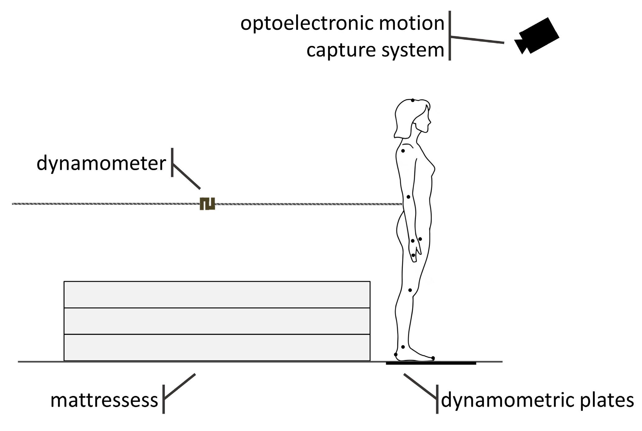
In this study, a healthy female, aged 25, was asked to perform several movement patterns—front and back swings with her arms while standing still and a backward fall. The movements were captured with the use of the BTS Smart motion capture system (a sampling frequency of 250 Hz and a spatial measurement resolution of 0.001 m) complemented by two dynamometric AMTI plates with a sampling frequency of 500 Hz and a measurement resolution of 0.001 N. With the use of platforms, the ground reaction forces (GRF) and the centre of pressure (COP) trajectory were captured. The test participant stands with both feet on the platforms in an upright position, waiting for an impulse that will disturb their balance. After a possible defence against a fall, they return to the starting position. Recording starts in advance to register the stationary position of the subject as well. Additionally, the external random force was applied to the participant’s body to cause a backward fall. The time course of the external force was registered with the use of a dynamometer whose sampling frequency and measurement resolution are equal to 500 Hz and 0.5 N, respectively. Since the dynamometer was an external device, its signal was synchronized with the data obtained with the use of platforms and a motion capture system through software. The raw data approximation algorithm, described in Section 5, solves the problem of the different sampling frequencies of the measured signals. The schematic view of the experimental setup is shown in Figure 1. The participant was standing on the platforms with each foot on a separate platform. They were asked not to move their feet during the exercise. During the registration of the motion, the main sagittal plane of the person remains parallel to the XZ plane. To ensure safety while performing external force-caused falls the mattresses were put behind the participant.
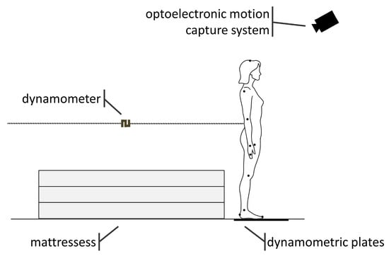
Figure 1.
Diagram of the experimental setup (right-hand view in the XY-plane).
To capture the body position during the exercises, passive markers were placed on the body of the subject. Shown in Figure 2, the placement of nineteen passive markers on the surface of a person’s body results from the assumptions of the Dempster model about the division of the human body into segments. Moreover, two markers attached to the rope make it possible to define the direction of the external force.
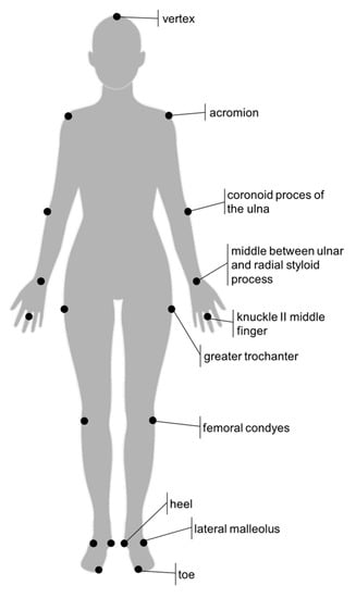
Figure 2.
Placement of passive markers on the subject’s body.
3. Human Body Biomechanical Model
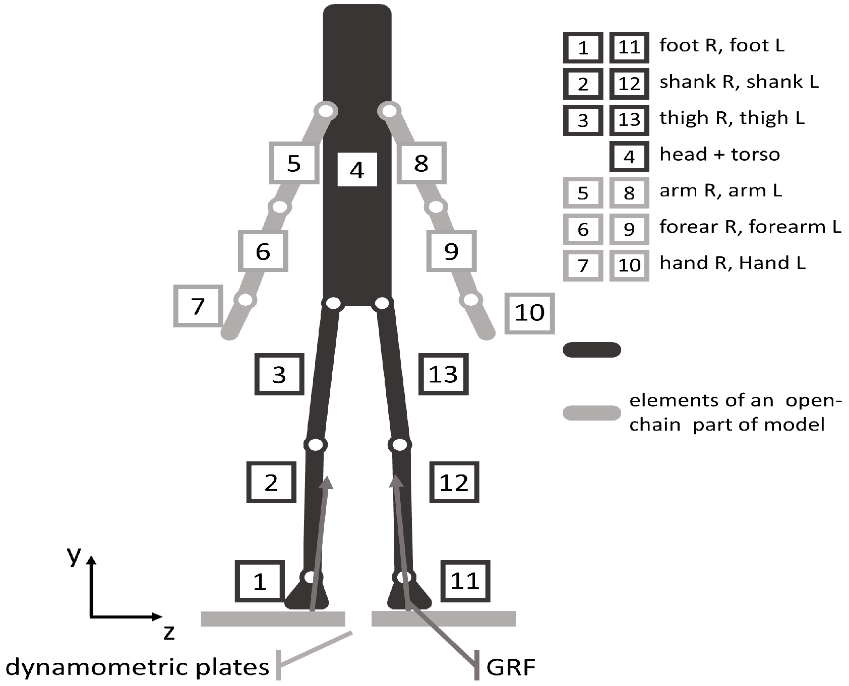
The two-dimensional biomechanical model proposed is based on the Dempster model, for which the inertial properties are defined in [14]. The model consists of 13 parts corresponding to the main human body segments. The upper limb divides into the arm, forearm, and hand. The foot, shank, and thigh are elements of the lower limb. One element called further the torso represents the trunk, head, and neck. All the parts of the model are assumed to be rigid bodies. The segments are numbered from one to thirteen. The numbering approach, shown in Figure 3, is important due to the system of denotations that we have introduced to distinguish mechanical quantities corresponding to particular body segments.
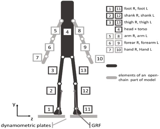
Figure 3.
Front view (in the plane XY) on the biomechanical model.
The characteristic dimensions of the segments, including the lengths of the limb parts denoted by , where are calculated according to the position of markers attached to bony prominences on the body. The mass of each segment, is defined as the percentage of total body mass accordingly to the anthropometric Dempster data. Due to the symmetry of the body segments assumed, their centres of mass lie on the individual axes of symmetry passing through the joints. Only the case of the torso’s centre of mass is different—there the centre lies on the line of symmetry. In the case of limb segments, the location of the centre of mass is defined by the distance measured from the proximal joint. The distances between the centre of mass of the torso and the greater trochanter and the acromion are denoted by and respectively. All the distances mentioned are specified relative to the segment length accordingly to Dempster’s data. The exception to this rule is the method of determining the position of the centre of mass of the foot. Taking into account the shape of the foot, a more adequate model seems to be a triangle whose vertices correspond to the markers of the side ankle, toe and heel. Thus, the centre of mass of the foot was taken at the centre of mass of this triangle. The mass moments of inertia of particular segments about the axes that pass through the centres of mass and are perpendicular to the sagittal plane are needed. The radii of gyration, given by Dempster in the relative form, are used to calculate these quantities. The values of mass and mass moments of inertia of individual segments of the person doing exercises are specified in Table 1.

Table 1.
Values of mass and mass moments of inertia of particular body segments of the person performing exercises.
The body segments are assumed to be connected by revolute joints (also called hinge or pin joints). These model joints correspond to the main joints of the human skeletal system, although due to the assumption of the planar motion of the biomechanical model, they do not always reflect the actual mobility of a given joint. There are 12 revolute joints in the model. Musculoskeletal interactions between two segments connected by a joint are modelled by a force and a couple at a given joint. Passing through the joints on the right side from the right foot to the right hand, we encounter a situation in which the indexes of the body segments are arranged in ascending order. Then, the internal force and couple at the joint linking the ith body segment with the (i+1)th segment receive the lower of the two indexes. The internal forces and couples at the joints of the left upper limb are subscripted from seven to nine, and the numbering starts from the shoulder joint. In turn, the subscripts assigned to internal forces and couples at the joints of the left lower limb change from 10 to 12, starting from the ankle joint. The force , where is resolved into two rectangular components parallel to and axes. The couples accompanying them are represented by the moments that are perpendicular to the YZ-plane Thus, we can write that and
External loads of the model include the forces of gravity of individual body parts, the ground reaction forces measured with the dynamometric plates, and the force disturbing the equilibrium position and registered via the dynamometer. The force of gravity of the ith body segment is assumed to act at the mass centre and be equal to , where stands for the acceleration of the Earth.
During the back-to-front arms swings as well as during the exercise involving the backward fall, the person doing these exercises stands with both feet on the dynamometric platforms. Thus, the biomechanical model reflecting these activities can be regarded as a closed kinematic chain with one loop, including the lower limbs and the torso. Two open kinematic subchains corresponding to the upper limbs are attached to this loop.
4. Mathematical Model
The current configuration of the considered biomechanical system is uniquely determined by 13 angles φi that are measured counterclockwise in the sagittal plane (i.e., YZ-plane). A rule was adopted in the paper that the directed angle φi is measured from the horizontal axis of the own local system, which is parallel to the Z axis, to the symmetry axis of the given segment. The time derivatives φi of the angles φi stand for the angular velocities of the segments, and the second derivatives are their angular accelerations. The Newton–Euler approach requires the introduction of quantities defining the kinematic state of the centres of mass of each body segment. Let yi and zi be the Cartesian coordinates of the mass centre Ci within the global coordinate system OXYZ. Differentiating the coordinates over time, we get the Cartesian components of the velocities of the mass centres. Differentiating twice yields the Cartesian components of the accelerations of the mass centres. Since the dimensions of model parts are described by angles and distances from the centre of mass of the current segment, the initial state of the examined person does not affect the results.
Within the framework of the two-dimensional problem, we write three equations of motion for each of the parts of the biomechanical model. The first two of them result from the first Euler’s law. The third equation, resulting from the second Euler’s law, concerns the angular momentum around the mass centre.
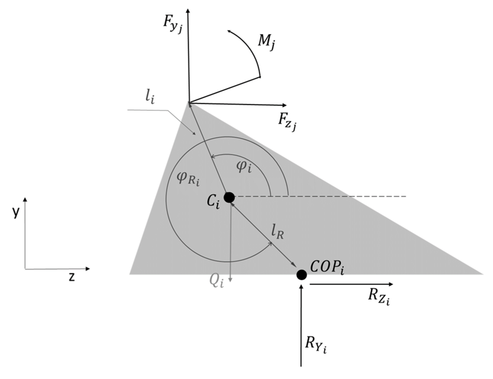
For feet whose free-body diagram is shown in Figure 4, the equations are as follows:
where for the right foot and for the left foot.

Figure 4.
Foot model sketch (identical for left and right foot). The symbols stand for: i—segment number, which takes the value of 1 or 11 (according to Figure 3), li—the distance between the centre of mass of the foot (Ci) and the ankle joint, the distance between the centre and the centre of pressure COP, —the directed angle that defines the location of the segment joining the centres of mass and pressure, and , —components of the reaction forces.
The free-body diagrams for shanks, thighs, arms, and forearms differ only in symbol indices. Therefore, we present all these diagrams only once in Figure 5.
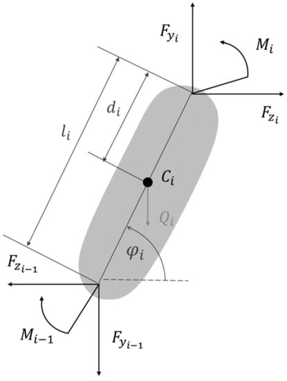
Figure 5.
Free-body diagram representative for the segments standing for shanks, thighs, arms, and forearms. The symbols used mean: i—segment number, which takes one of the following values: 2, 3, 5, 6, 8, 9, 12, 13 (according to Figure 3), li—length of the ith segment, and di—distance from the end of the ith segment, which connects to the i+1 segment, to the segment’s centre of mass (Ci).
According to Figure 5, the equations of motion for the limbs segments have the following form:
where .
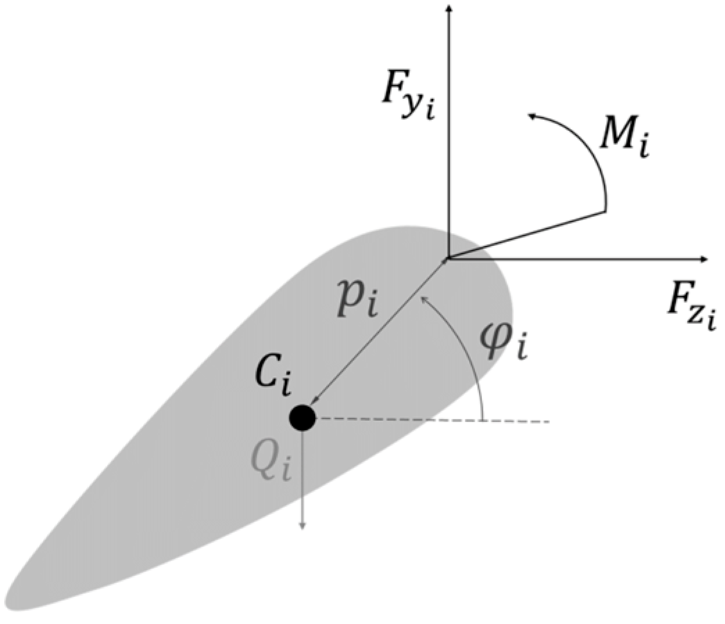
Hands, as peripheral parts of the model, are characterized by a simple load scheme shown in Figure 6.

Figure 6.
The free-body diagram for both hands. Used symbols stand for: i—segment number, which takes the value of 7 or 10 (according to Figure 3), and pi—the distance from the proximal end of the segment to the segment’s centre of mass (Ci).
The equations of motion for both segments representing hands take the following form:
where for the right hand, and for the left hand.
The external force , which disturbs randomly the equilibrium position, is exerted on the torso. We assume that it acts at a point whose position relative to the mass centre is specified by the segment of length and the directed angle . The directed angle , depicted along with other elements in Figure 7, determines the direction of the force relative to the horizontal line. The equations governing the motion of the part corresponding to the torso are as follows:
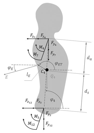
Figure 7.
The free-body diagram for the segment representing the head and torso. stands for the external force applied to the participant.
The motion of the biomechanical model in the sagittal plane is described by the set of 39 ordinary differential equations of the second order with known geometrical and mass parameters. The forces of gravity are also a priori known. In the experiment, we measure the ground reaction forces and the external force that is supposed to induce a backwards fall. The registration of passive markers’ positions allows for indirect determination of the positions of the model segments, their angular accelerations, and linear accelerations of the mass centres. By substituting the measured forces and indirectly determined kinematic quantities into the equations of the mathematical model, one can determine the values of forces and moments of couples at the joints. There are 36 unknowns within the framework of the formulated inverse dynamic problem. Since the feet stand on separate dynamometric platforms, the information about the GRF and COP for both lower limbs can be used in the calculations. Thereto, the number of equations is greater than the number of unknowns. The values of the GRF and COP, obtained from the platform on which the right leg supports, are the input data. Analogous values obtained from the second platform can serve to validate the model and calculating procedure.
5. Data Preparation
Knowing the current coordinates of the passive markers, one can determine the values of the angles . The local horizontal axes, from which the directed angles are measured, are depicted in Figure 4, Figure 5, Figure 6 and Figure 7. Except for the feet and hands, they pass through one of the joints belonging to the given body segment. The auxiliary horizontal axes that are needed to define the angles for hands and feet pass through the appropriate mass centre. Let the points through which all the auxiliary horizontal axes pass be the origins of the local coordinate systems. Denoting by and the coordinates of the opposite joint within the given local system, we can determine the directed angle employing the following formulas:
The Cartesian coordinates of the centres of mass are calculated based on the coordinates of the markers with the use of Dempster’s data.
The linear and angular accelerations are not measured directly in the experiment. It is, therefore, necessary to determine all the acceleration approximately based on the calculated values of the Cartesian coordinates and directed angles . These quantities are affected by measurement error and random disturbances, including marker displacements caused by breathing movements and cameras’ stand vibrations.
To smooth the raw data and determine the derivatives needed, we applied a variant of function approximation. The method enables the simultaneous approximation of a function and its first and second derivatives. Let be any real-valued function of one variable that is smooth together with its derivatives of the first and second orders. Only approximate values of the function are known at points that are uniformly distributed over the interval . Let be a subinterval with a centre at point , where is an integer number. We approximate the function on the subinterval by the polynomial of the form
where are unknown coefficients. Calculating the first and second derivatives of the polynomial , we obtain:
When the argument takes the value , then
From relationship (17) results that the unknown coefficients depict the estimated values of the function and its both derivatives at the middle point of the subinterval , i.e.,
We define the following functional:
where are the measured values of the function . The functional depicts the total absolute squared error of the function approximation on the subinterval .
Substituting definition (14) into Equation (19) yields
The sought coefficients, , can be uniquely determined by solving the set of three linear equations expressing the necessary conditions of existence of the extremum of the function These equations have the following form:
6. Results
After developing the biomechanical and mathematical model, and designing the experimental setup along with the detail concerning the carrying up measurements, we conducted several experiments with the participation of a healthy female aged 25. We expanded the scope of the experiment to include exercises involving swinging the upper limbs while standing on two platforms. Such movements can also be described in the framework of the model that we propose when assuming that the external force does not act. Upper limb swings are routine defensive behaviours of people at risk of an incidental fall. An exercise in which only the upper limbs are active gives the possibility to test the sensitivity of the measurement method and calculation procedure to arm swings, which are unavoided during the experiments being the main subject of research on the loss of a stable body position.
The experiments performed are aimed at testing the research method, detecting its weaknesses, and specifying the factors affecting the accuracy of results. As mentioned in Section 4, the use of two dynamometer platforms provides the opportunity to evaluate the method by comparing the reaction force quantities for the left foot with their measured counterparts. In this section, we present and discuss only the results of this comparison.
For the quantitative assessment of the global error, which is affected by measurement errors, simplifying model assumptions, the uncertainty of inertial parameters and errors in the algorithm for determining kinematic quantities, the following relative measure, based on the metric in Euclidean space, is used
where stands for the measured value of the component of the reaction force at instant, is the value of the component calculated from the mathematical model, and n denotes the number of measured values.
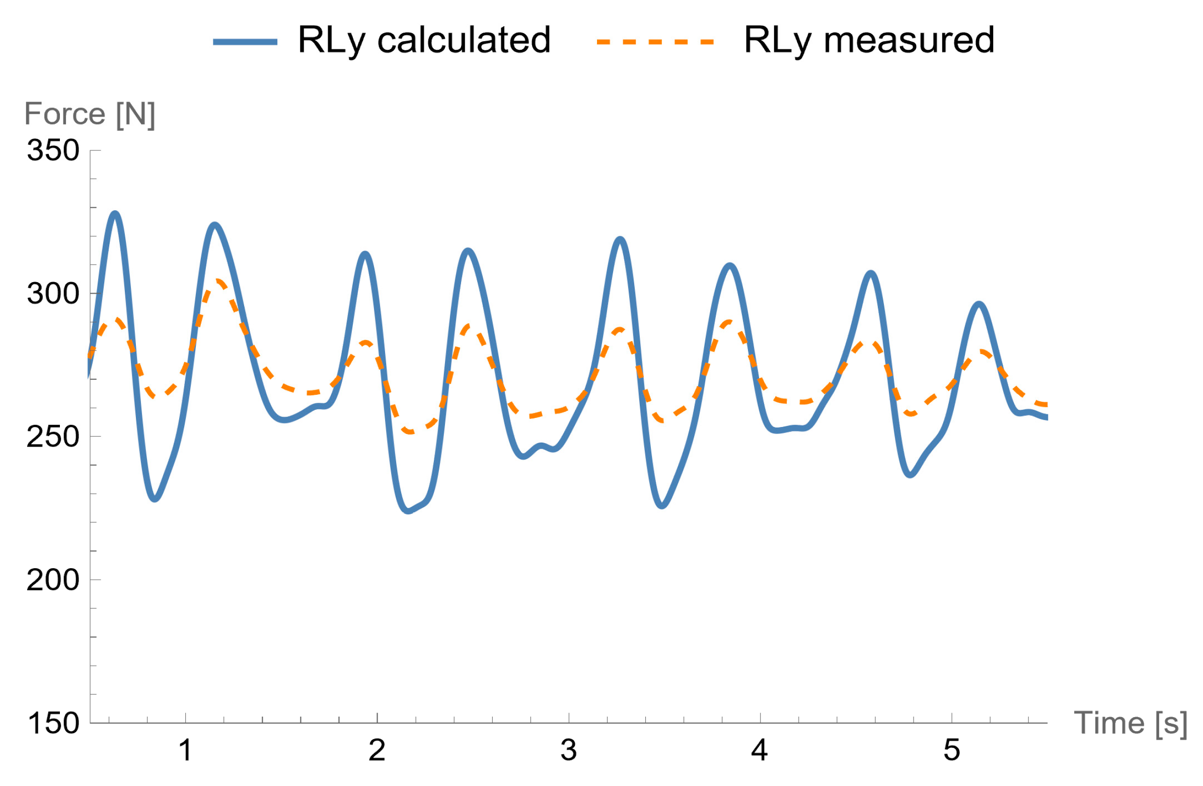
We start the discussion with the results concerning the exercise with swinging of upper limbs back and forth at the standing position. Figure 8 shows the time course of the vertical component of the ground reaction force acting on the left foot. The graph prepared based on the measured values (after the necessary approximation) is drawn with a dashed line. The solid line shows the waveform obtained as a result of solving the equations of the mathematical model. The qualitative nature of both time courses is consistent. However, differences in the values of both functions can be observed. The peak-to-peak values are smaller for the vertical component obtained from the measurement.
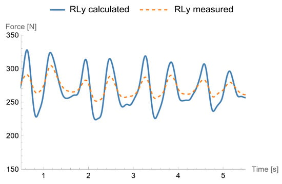
Figure 8.
The vertical component, RLy, of the GRF for the left foot in the case of the exercises with upper limbs swinging. The RLy measured with the dynamometric plate is drawn using the dashed line, and the RLy calculated is drawn using the solid line. The error δ = 0.0841.
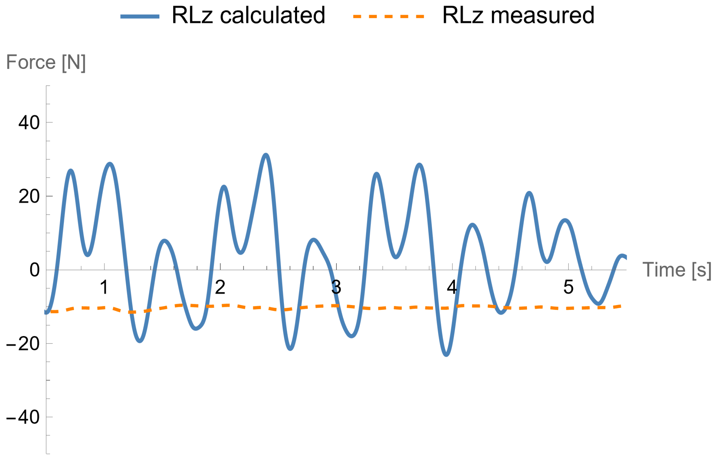
Figure 9 shows, using the same method of presentation, the time course of the horizontal component of the GRF for the left foot. Although one can still notice the agreement manifested by reaching extreme values at the same time, the differences between the two graphs are significant both quantitatively and qualitatively. The observation of a much smaller range of changes between the peaks for the directly registered signal is confirmed.
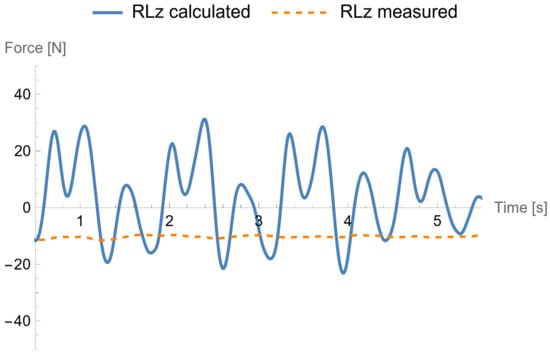
Figure 9.
The horizontal component, RLz, of the GRF for the left foot in the case of the exercises with upper limbs swinging. The RLz measured with the dynamometric plate is drawn using the dashed line, and the RLz calculated is drawn using the solid line.
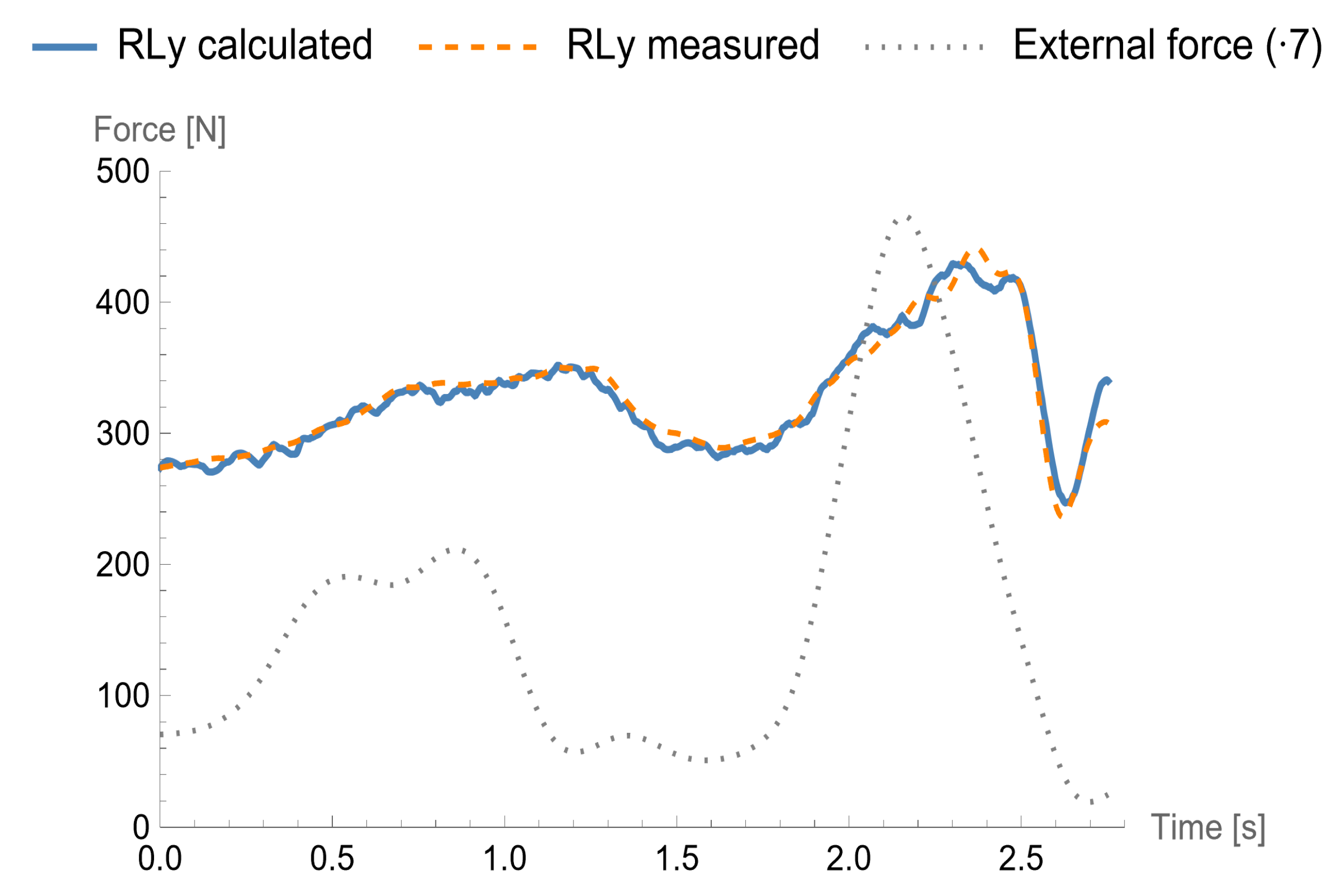
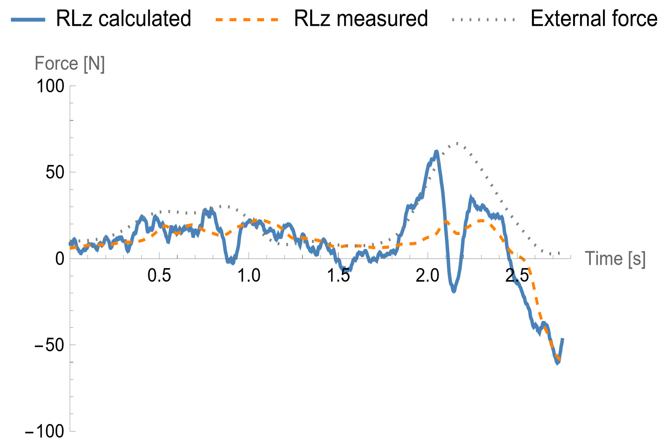
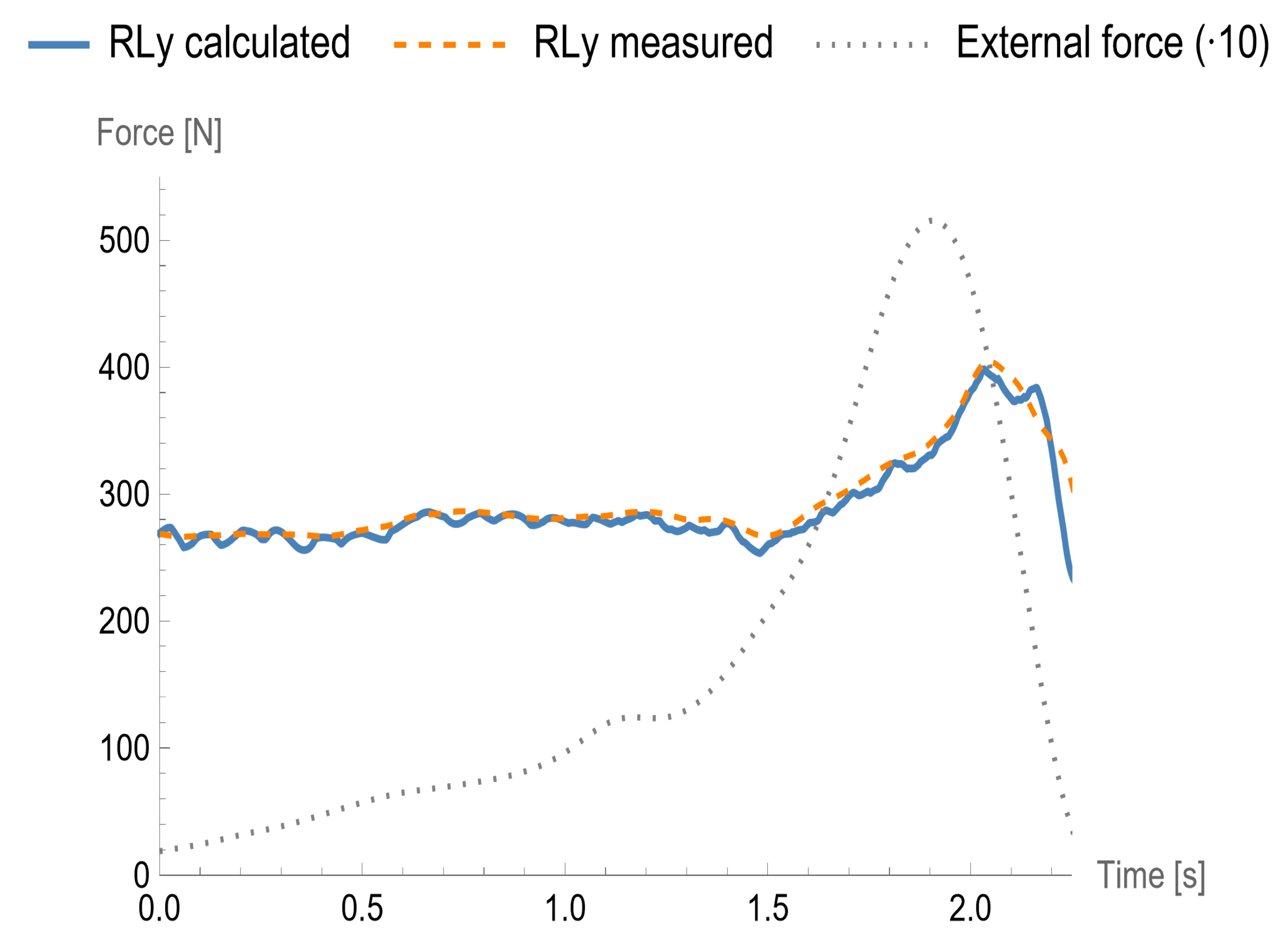
Exercises with the external force causing a fall backwards differ in the number of pulls registered by the dynamometer. One or two pulls of varying strength and random timing were exerted on the participant. The time history of the magnitude of the external force is shown in each of Figure 10, Figure 11, Figure 12 and Figure 13 using the dotted line. The results shown in Figure 10 and Figure 11 refer to the fall when the participant was pulled twice. They show the vertical and horizontal components of the GRF versus time, respectively. The first pull was too mild, and the participant was able to maintain balance. The second pull ended up with a fall. The time courses of the measured (dotted line) and calculated (solid line) vertical components of the GRF are almost consistent. The in-plane components differ to a greater extent. One can note that the graphs based on the calculated quantities have a more oscillatory nature, which may be related to the ill-conditioned problem of determining derivatives of kinematic quantities. The last remark applies especially to the horizontal component.
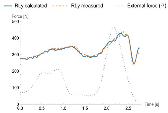
Figure 10.
The vertical component, RLy, of the GRF for the left foot in the case of the external force-caused fall with two pulls. The RLy measured with the dynamometric plate is drawn using the dashed line, and the RLy calculated is drawn using the solid line. The dotted line presents the time course of the external force magnitude. The error δ = 0.0227.
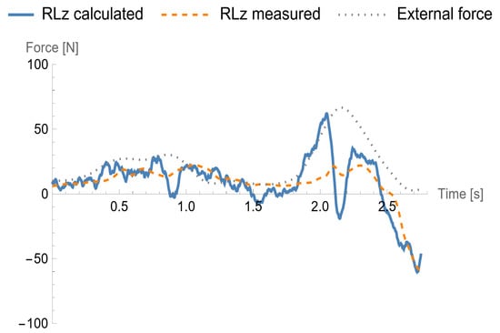
Figure 11.
The in-plane component, RLz, of the GRF for the left foot in the case of the external force-caused fall with two pulls. The RLz measured with the dynamometric plate is drawn using the dashed line, and the RLz calculated is drawn using the solid line. The dotted line presents the time course of the external force magnitude.
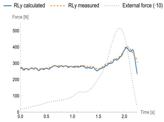
Figure 12.
The vertical component, RLy, of the GRF for the left foot in the case of the external force-caused fall with a single pull. The RLy measured with the dynamometric plate is drawn using the dashed line, and the RLy calculated is drawn using the solid line. The dotted line presents the time course of the external force magnitude. The error δ = 0.0248.
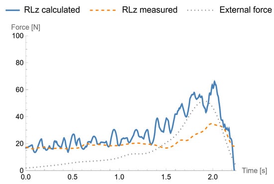
Figure 13.
The vertical component, RLy, of the GRF for the left foot in the case of the external force-caused fall with a single pull. The RLy measured with the dynamometric plate is drawn using the dashed line, and the RLy calculated is drawn using the solid line. The dotted line presents the time course of the external force magnitude.
We also observe a high agreement between the courses of the vertical components, measured (dashed line) and calculated from the equations of the mathematical model (solid line), which are shown in Figure 12, and which refer to the fall that occurred after one strong pull with the rope. Unfortunately, both waveforms of the horizontal components of the GRF, shown in Figure 13, do not show such an agreement.
7. Discussion
Employing the approach described above, one can determine the time courses of the forces and couples at human joints that act during an incidental fall backwards. The values of the internal forces are important for assessing the effects of these falls. At the same time, the knowledge of the loads in the joints in dynamic conditions allows for a more accurate study of the causes and scenarios of loss of stability compared to an analysis based solely on the equations of statics. At this stage, after developing a biomechanical and mathematical model, designing an experiment and conducting a short test series of measurements, we focused on validating the method and model. Experiments with two dynamometric platforms enable such validation by comparing the waveforms of the components of the GRF for one of the feet (here, it is the left foot) with the measured values.
Comparing obtained results for various movement patterns, it can be noticed that the least accurate outcomes are obtained in the case of the exercise with arm swings (Figure 6 and Figure 7). In this movement, the inertial parameters of the upper limbs have the strongest impact on model error. Moreover, considering the quality of every data that were taken to the equations: accelerations, inertial and mass parameters, COP and GRF, the least accurate data seem to be the mass of the body segments and their inertial parameters. To estimate the aforementioned mass parameters, included in Table 1, the simple equations given by Dempster were used. Every mass or inertial parameter is defined as a percentage of body weight or segment length—without taking into account the differences in the construction of subsequent parts of the body. The significant influence of inertial parameters on the accuracy of the model can also be noticed in the waveform of the horizontal component of GRF referring to the force-caused falls (Figure 9 and Figure 11). The greatest differences between the measured and calculated GRF components were observed when an external force was applied to the body and the body segments moved in response to the disturbance with high accelerations. While the movement became slower, the calculated values of the GRF started to match again to the measured GRF. The model also works better for the horizontal than vertical GRF estimation—this also is caused by the influence of the inertial parameters, because the movement in the horizontal direction (i.e., along the Z axis) is dominant.
Future studies will focus on the extension of the research to a larger group of participants to confront the outcomes obtained for people with different silhouettes. In addition, a study on better estimation of mass and inertial parameters should be performed, since the outcomes of our preliminary research demonstrate a high influence of those parameters on the efficiency of the model. Moreover, a more detailed study should be conducted on inertial parameters to expand the model to the three-dimensional space.
However, taking into account the high accuracy of the model, especially in vertical GRF, it can be stated that the presented two-dimensional model for external force-caused fall analysis can be used as a basis to perform further research.
Author Contributions
Designing and conducting an experiment, calculations and data preparation, writing, M.S.; mathematical model development, supervision, writing G.S.-K.; supervision, writing, T.W., supervision, mathematical model development, H.K. All authors have read and agreed to the published version of the manuscript.
Funding
This research was funded by grant 0612/SBAD/3588 of the Ministry of Science and Higher Education.
Institutional Review Board Statement
Ethical review and approval were waived for this study because participants in the study were also authors of the study.
Informed Consent Statement
Patient consent was waived because the participant in the study was also an author of the study.
Conflicts of Interest
The authors declare no conflict of interest.
References
- World Health Organization. WHO Global Report on Falls Prevention in Older Age; World Health Organization: Geneva, Switzerland, 2007. [Google Scholar]
- Grivna, M.; Eid, H.O.; Abu-Zidan, F.M. Epidemiology, morbidity and mortality from fall-related injuries in the United Arab Emirates. Scand. J. Trauma Resusc. Emerg. Med. 2014, 22, 51. [Google Scholar] [CrossRef]
- Mroczkowski, A. Susceptibility to Head Injury during Backward Fall with Side Aligning of the Body. Appl. Sci. 2020, 10, 8239. [Google Scholar] [CrossRef]
- Elvik, R. Risk of non-collision injuries to public transport passengers: Synthesis of evidence from eleven studies. J. Transp. Heal. 2019, 13, 128–136. [Google Scholar] [CrossRef]
- Kerber, K.A.; Bi, R.; Skolarus, L.E.; Burke, J.F. Trajectories in physical performance and fall prediction in older adults: A longitudinal population-based study. J. Am. Geriatr. Soc. (JAGS) 2022, 70, 3413–3423. [Google Scholar] [CrossRef] [PubMed]
- Howcroft, J.; Lemaire, E.D.; Kofman, J.; McIlroy, W.E. Elderly fall risk prediction using static posturography. PLOS ONE 2017, 12, e0172398. [Google Scholar] [CrossRef]
- Savadkoohi, M.; Oladunni, T.; Thompson, L. Deep neural networks for human’s fall-risk prediction using force-plate time series signal. Expert Syst. Appl. 2021, 182, 115220. [Google Scholar] [CrossRef] [PubMed]
- Walczak, T.; Sopa, M.; Pogorzała, A. Application of Artificial Neural Networks in Fall Prediction. Vib. Phys. Syst. 2021, 32, 2021210-1–2021210-8. [Google Scholar] [CrossRef]
- Xu, Q.; Huang, G.; Yu, M.; Guo, Y. Fall prediction based on key points of human bones. Phys. A Stat. Mech. its Appl. 2019, 540, 123205. [Google Scholar] [CrossRef]
- Howcroft, J.; Lemaire, E.D.; Kofman, J. Prospective elderly fall prediction by older-adult fall-risk modeling with feature selection. Biomed. Signal Process. Control. 2018, 43, 320–328. [Google Scholar] [CrossRef]
- Da Conceição, N.R.; de Sousa, P.N.; Pereira, M.P.; Gobbi, L.; Vitório, R. Utility of center of pressure measures during obstacle crossing in prediction of fall risk in people with Parkinson’s disease. Hum. Mov. Sci. 2019, 66, 1–8. [Google Scholar] [CrossRef]
- Saleh, M.; Abbas, M.; Le Jeannes, R.B. FallAllD: An Open Dataset of Human Falls and Activities of Daily Living for Classical and Deep Learning Applications. IEEE Sens. J. 2020, 21, 1849–1858. [Google Scholar] [CrossRef]
- Peng, Y.; Peng, J.; Li, J.; Guo, L.; Hu, B.; Wang, Z. A Human Fall Detection Method based on Machine Learning and TRIZ Theory. Elektrotehniški Vestn. 2020, 87, 117–126. [Google Scholar]
- Winter, D.A. Chapter 9: Kinesiological Electromyography. In Biomechanics and Motor Control of Human Movement, 3rd ed.; Winter, D.A., Ed.; John Wiley & Sons, Inc.: Hoboken, NJ, USA, 2005. [Google Scholar]
- Dumas, R.; Wojtush, J. Estimation of the Body Segment Inertial Parameters for the Rigid Body Biomechanical Models Used in Motion Analysis. In Handbook of Human Motion; Springer: Cham, Switzerland, 2018; pp. 47–77. [Google Scholar]
- Cerda-Lugo, A.; González, A.; Cardenas, A.; Piovesan, D. Modeling the neuro-mechanics of human balance when recovering from a fall: A continuous-time approach. Biomed. Eng. Online 2020, 19, 1–24. [Google Scholar] [CrossRef]
- Hettich, G.; Fennell, L.; Mergner, T. Double Inverted Pendulum Model of Reactive Human Stance Control, Multibody Dynamics. In Proceedings of the ECCOMAS Thematic Conference, Brussels, Belgium, 4–7 July 2011. [Google Scholar]
- Zhou, X.; Liu, G.; Han, B.; Wu, L.; Li, H. Design of a Human Lower Limbs Exoskeleton for Biomechanical Energy Harvesting and Assist Walking. Energy Technol. 2020, 9, 2000726. [Google Scholar] [CrossRef]
- Berret, B.; Darlot, C.; Jean, F.; Pozzo, T.; Papaxanthis, C.; Gauthier, J.P. The Inactivation Principle: Mathematical Solutions Minimizing the Absolute Work and Biological Implications for the Planning of Arm Movements. PLoS Comput. Biol. 2008, 4, e1000194. [Google Scholar] [CrossRef]
- Grzelczyk, D.; Biesiacki, P.; Mrozowski, J.; Awrejcewicz, J. A 4-Link of a Human for Simulating a Forward Fall. Vib. Phys. Syst. 2018, 29, 2018008. [Google Scholar]
- Meng, Q.; Lai, X.; Yan, Z.; Su, C.-Y.; Wu, M. Motion Planning and Adaptive Neural Tracking Control of an Uncertain Two-Link Rigid–Flexible Manipulator With Vibration Amplitude Constraint. IEEE Trans. Neural Networks Learn. Syst. 2021, 33, 3814–3828. [Google Scholar] [CrossRef] [PubMed]
- Lu, S.; Ban, Y.; Zhang, X.; Yang, B.; Liu, S.; Yin, L.; Zheng, W. Adaptive control of time delay teleoperation system with uncertain dynamics. Front. Neurorobotics 2022, 16. [Google Scholar] [CrossRef] [PubMed]
- Avilov, A.V.; Avilova, N.V.; A Krivtsov, I. Simulation Biomechanical Modeling of Human Walking. J. Physics: Conf. Ser. 2020, 1443, 012020. [Google Scholar] [CrossRef]
- Biesiacki, P.; Mrozowski, J.; Grzelczyk, D.; Awrejcewicz, J. Modelling of Forward Fall on Outstretched Hands as a System with Ground Contact. In Dynamical Systems: Modelling; Awrejcewicz, J., Ed.; DSTA 2015; Springer Proceedings in Mathematics & Statistics; Springer: Cham, Switzerland, 2016; Volume 181, pp. 61–72. [Google Scholar] [CrossRef]
- Kuo, A. A Least-Squares Estimation Approach to Improving the Precision of Inverse Dynamics Computations. J. Biomech. Eng. 1998, 120, 148–159. [Google Scholar] [CrossRef]
- Dasgupta, B.; Choudhury, P. A general strategy based on the Newton–Euler approach for the dynamic formulation of parallel manipulators. Mech. Mach. Theory 1999, 34, 801–824. [Google Scholar] [CrossRef]
- Price, M.A.; LaPrè, A.K.; Johnson, R.T.; Umberger, B.R.; Sup, F.C. A model-based motion capture marker location refinement approach using inverse kinematics from dynamic trials. Int. J. Numer. Methods Biomed. Eng. 2019, 36, e3283. [Google Scholar] [CrossRef] [PubMed]
- Venne, A.; Bailly, F.; Charbonneau, E.; Dowling-Medley, J.; Begon, M. Optimal estimation of complex aerial movements using dynamic optimisation. Sports Biomech. 2022, 22, 300–315. [Google Scholar] [CrossRef] [PubMed]
Disclaimer/Publisher’s Note: The statements, opinions and data contained in all publications are solely those of the individual author(s) and contributor(s) and not of MDPI and/or the editor(s). MDPI and/or the editor(s) disclaim responsibility for any injury to people or property resulting from any ideas, methods, instructions or products referred to in the content. |
© 2023 by the authors. Licensee MDPI, Basel, Switzerland. This article is an open access article distributed under the terms and conditions of the Creative Commons Attribution (CC BY) license (https://creativecommons.org/licenses/by/4.0/).

