Short-Term Bus Passenger Flow Prediction Based on Graph Diffusion Convolutional Recurrent Neural Network

Featured Application

This study integrates diffusion convolution in a graph into a recurrent neural network to capture the spatiotemporal dependencies of different bus lines in a bus network for better passenger flow prediction. The proposed method is implemented in the bus network of Jiading, Shanghai, and achieves better modeling performance than that of the classic recurrent neural network models.

Abstract

The short-term bus passenger flow prediction of each bus line in a transit network is the basis of real-time cross-line bus dispatching, which ensures the efficient utilization of bus vehicle resources. As bus passengers transfer between different lines, to increase the accuracy of prediction, we integrate graph features into the recurrent neural network (RNN) to capture the spatiotemporal dependencies in the bus network. The diffusion convolution recurrent neural network (DCRNN) architecture is adopted to forecast the future number of passengers on each bus line. The demand evolution in the bus network of Jiading, Shanghai, is investigated to demonstrate the effectiveness of the DCRNN model. Compared with classic RNN models, our proposed method has an advantage of about 5% in mean average percentage error (MAPE). The incorporation of diffusion convolution shows that the travel demand in a bus line tends to be similar to that in the closely related lines. In addition, the improvement in MAPE shows that this model outputs more accurate prediction values for low-demand bus lines. It ensures that, for real-time cross-line bus dispatching with limited vehicle resources, the low-demand bus lines are less likely to be affected to maintain a decent level of service of the whole bus network.

1. Introduction

The rapid progress of urbanization and the fast growth of urban populations has led to a series of roadway transport problems such as severe traffic congestion [1]. The surge in traffic volume then seriously affects the normal operation of bus transit services. For bus transit operators, the real-time control strategies of bus operations, such as cross-line bus dispatching, has become one of the most effective means to reduce disturbance during operation [2]. The cross-line dispatching strategy involves allocating bus vehicles from low-demand bus lines to high-demand ones to match the peak bus travel demand in a bus transit network. The basis of this real-time strategy is the short-term prediction of passenger flows [3]. With the accurate prediction of passenger flows, especially in low-demand bus lines, the operations of bus transit services can be more effective and efficient, thereby enhancing the attractiveness of the whole public transit service [4,5]. With more travelers shifting to the public transit system, it can ultimately mitigate traffic congestion, leading to the sustainable development of the city.

With the development of the smart integrated circuit (IC) card system, bus transit operators are able to collect the bus travel demand in real-time [6]. Thus, a series of data-driven methodologies have been developed for travel demand prediction. Early studies paid more attention to time series analyses. For instance, Ahmed et al. [7] utilized an autoregressive integrated moving average (ARIMA) model for short-term travel demand forecasting. Williams et al. [8,9] developed the theoretical foundation for travel demand prediction using the seasonal ARIMA process. Li et al. [10] proposed an improved ARIMA-based prediction method to forecast the spatial–temporal variation in passengers. In addition to the time series analyses, the Kalman filter, known for its robustness against the noise in data, has also been widely used for prediction tasks. For example, Jiao et al. [11] modified the traditional Kalman filter based on the error correction coefficient, historical deviation, and Bayesian combination to predict short-term passenger flows in the rail transit system. Nonetheless, these statistical methods normally assume that the changes in travel demand are linear, whereas the actual patterns may be nonlinear. To overcome this limitation, various machine learning models have been applied for travel demand forecasting.

Classic machine learning methods, such as support vector regression [12] and K-nearest neighbor [13], have been widely used to transform time series problems into supervised learning problems, which achieve a high prediction accuracy. Toqué et al. [14] proposed to use random forest models to predict the number of passengers entering each metro station or boarding at each bus stop. Li et al. [15] developed a secondary decomposition integration method that combines empirical modal decomposition, sample entropy, and kernel extreme learning machines for the short-time prediction of bus route passenger flow. However, the shallow structure of the classic machine learning methods makes it difficult to handle the complex non-linearity in spatial and temporal patterns of travel demand [16].

In recent years, deep learning models have been widely applied to prediction problems in the transportation field. To deal with the temporal dependency, Gang et al. [17] adopted a deep neural network to predict continuous travel time for transit signal priority. Ma et al. [18] used a recurrent neural network for traffic speed prediction, while Duan et al. [19] employed the long short-term memory (LSTM) model for travel time prediction. For travel demand prediction, Huang et al. [20] proposed a deep architecture composed of deep belief networks (DBN) and multitask regression layers for short-term travel demand prediction. Ke et al. [21] developed a short-term passenger demand prediction method based on the LSTM to capture the temporal features, of which the results show that the deep learning models outperform the classic machine learning methods.

In addition to temporal dependency, the spatial relationship pertains to the utilization of neighboring data to enhance the effectiveness of deep learning. By scanning a filter across the grid-structured data, the convolutional neural network (CNN) structure is developed to capture the neighborhood features [22,23]. Nonetheless, with non-grid data structures, such as graphs, the graph convolutional network (GCN) has an advantage over CNN by considering the connectivity information between the vertices in the graph [24]. For instance, Yu et al. [25] have proposed a spatiotemporal GCN model that does not use traditional conventional units but constructs a model on a graph instead to address the time series prediction problems.

Since then, more studies have started to take into account both temporal and spatial dependencies for travel demand prediction. Polson et al. [26] proposed a deep learning architecture to capture nonlinear spatiotemporal effects. Liu et al. [27] modeled the periodicity of travel demand and the spatial correlation between metro stations with the incorporation of factors, such as weather and holidays, to perform the short-term prediction of passenger flows in the metro system. Ren et al. [28] combined LSTM with spatiotemporal residual networks to predict the spatiotemporal travel flow across the city. Zhao et al. [29] proposed a graph-based deep learning approach by fusing the dynamic built environment influences and spatiotemporal dependency to predict short-term bus travel demand. Chen et al. [30] adopted the spatial–temporal graph sequence with the attention network for bus passenger flow forecasting in Urumqi, China. Baghbani et al. [31] developed a more scalable and robust bus network graph convolutional long short-term memory neural network model using data from the Laval bus network in Canada. These novel deep learning frameworks present great performance in capturing complicated spatiotemporal dependencies in travel demand prediction.

Most existing graph-based models, including the GCNs, typically view edges as simple binary connections, which are either present or absent. However, the real-world relationships between the vertices are often much more nuanced and intricate [32]. Thus, a new graph convolution method, the graph diffusion convolution (GDC), is developed upon the foundation of GCN [33]. In the process of GDC, the attention of the model is initially focused on one node of interest, then gradually spreading to the node’s neighboring vertices, thereby diffusing the attention away from the starting node of interest. Such a process leads to a more comprehensive and flexible understanding of the underlying graph structure [34]. Li et al. [35] have applied a diffusion convolutional recurrent neural network model by integrating the GDC into RNN, in order to predict the roadway traffic based on the traffic sensor data. The experiments show that the model outperforms the other baseline methods. Furthermore, based on the ride-hailing data from DiDi Chuxing, Wang et al. [36] applied the same DCRNN approach to predict the evolution of urban traffic by capturing the spatial–temporal dependencies of the urban road network, which presents good performance even under extreme weather conditions.

This work contributes to the current literature by transforming the bus network into a series of graphs and integrating diffusion convolution into a classic RNN prediction framework to capture the spatiotemporal relationships between different bus lines in a bus transit network. The diffusion convolution process captures the impacts of distance decay in a series of spatially correlated vertices in a network, thereby enhancing the performance of bus passenger flow prediction. Based on the constructed graphs, the DCRNN model is adopted for the short-term prediction of bus passenger flows in each bus line. The proposed model is implemented in the bus network of Jiading, Shanghai, with 10-month consecutive observations. The advantageous performance of the DCRNN model is demonstrated by comparing it to several classic machine-learning models.

The remainder of this paper is organized as follows. Section 2 introduces the structure of the DCRNN model. In Section 3, we describe the study area and the data used in this work. Section 4 presents the modeling results with a comparison to other classic models. In Section 5, we conclude this work.

2. Methods

We focus on predicting bus passenger flows on each bus line in the whole bus transit network. In addition to the temporal patterns, the spatial interaction also plays an essential role in bus passenger flow evolution due to the inter-line transfers in a bus network. Considering both spatial and temporal impacts, we integrate diffusion convolution [35,37]—that integrates diffusion processes into random walks on the graph—into a recurrent neural network to capture the spatiotemporal relationships. Thus, a DCRNN structure that absorbs the advantages over GCN and RNN is adopted for this spatiotemporal forecasting task. In this section, we describe how to use the DCRNN for the short-term bus passenger flow prediction problem in detail.

2.1. Modeling the Bus Passenger Flow Prediction Problem

The aim of bus passenger flow forecasting is to predict the total number of passengers waiting for each line, given the previously observed volume of smart card transactions. In this problem, N is used to represent the total number of bus lines.

To develop the topology of a bus transit network, we define a weighted undirected graph $G=\left(V,E,M\right)$ to represent the topology of the bus network. In graph $G$, $V$ is a set of vertices; $\left|V\right|=N$; $E$ is a set of edges; and $M\in {ℝ}^{N\times N}$ is a weighted adjacency matrix representing the proximity of vertices. Here, the matrix is defined based on the common stops between bus lines. Denote the volume of transit card transactions on $G$ as a graph signal $X\in {ℝ}^{N\times I}$, where $I$ is the number of features of each vertex (e.g., the number of passengers boarding at the bus stops, the length of bus lines, the number of bus stops, and the meteorological information, etc.).

Let $X^{\left(t\right)}$ represent the graph signal observed at time $t$. Thus, to look into the bus passenger flow forecasting problem, we aim to learn a function $\xi \left(\cdot \right)$ that maps $\delta$ historical graph signals to $o$ future graph signals, given graph $G$:

$$\left(X^{\left(t-\delta +1\right)},\dots ,X^{\left(t\right)};G\right)\stackrel{\xi \left(\cdot \right)}{\to }\left(X^{\left(t+1\right)},\dots ,X^{\left(t+o\right)}\right)$$

(1)

2.2. Graph Diffusion Convolution for Spatial Dependency Modeling

To capture the relationship between bus passenger flow observations in each bus line with a spatially structured dataset, the spatial dependency should be considered. Here, the spatial dependency is modeled by relating bus passenger flows to a diffusion process that explicitly captures the stochastic evolution of bus travel demand. By convolving the random walks (with a restart probability $p\in \left[\mathrm{0,1}\right]$) over the maximum $\tau$ nearest neighbors for each vertex, the diffusion step $Y$ can effectively capture the spatial relationship between the observations. The graph diffusion $\mathsf{\Xi }$ is defined by Equation (2) while the diffusion process is demonstrated in Figure 1. At each step $y\in \left\{0,\dots ,Y\right\}$, the model identifies the neighbors that are $y$-steps away from a node and calculates the transition matrices accordingly. Specifically, the graph diffusion $\mathsf{\Xi }$ is expressed as:

$$\mathsf{\Xi }=\sum _{y=0}^{\infty }p{\left(1-p\right)}^y{T}^y$$

(2)

where $y$ is the diffusion step and $T$ denotes the transition matrix, defined by $D^{-1}M$ with an adjacency matrix $M$ in Graph $G$ and a diagonal degree matrix $D$. Matrix $D$ is defined based on $M$ in which each diagonal element $d_{ii}=\sum _j{m}_{ij}$. To operationalize the diffusion process, a finite $Y$-step truncation is often utilized in practice, with trainable weights assigned to each step.

When training the model, probability $\theta$—which is a learnable parameter—is combined with transition matrices $T=D^{-1}M$ to construct the diffusion convolutional filter. The resulting operation of diffusion convolution over a graph signal $X\in {ℝ}^{N\times I}$ and a filter $h_{\theta }$ can be defined as:

$$X_{:,i}{\star }_G{h}_{\theta }=\sum _{y=0}^{Y-1}\left({\theta }_y{\left(D^{-1}M\right)}^y\right)X_{:,i}$$

(3)

where $i\in \left\{0,\dots ,I\right\}$; $\theta \in {ℝ}^{Y\times 1}$ are the parameters of the filter; $D=diag\left(M1\right)$ in which $1\in {ℝ}^N$ denotes an all-one vector; and $y$ is the diffusion step.

To capture the effects of upstream and downstream bus passenger flows, we need to take into account both forward and backward diffusion processes. Thus, the bidirectional diffusion convolution operation should be considered and defined as follows:

$$X_{:,i}{\star }_G{h}_{\theta }=\sum _{y=0}^{Y-1}\left[\left({\theta }_{y,1}{\left(D_{out}^{-1}M\right)}^y\right)X_{:,i}+\left({\theta }_{y,2}{\left(D_{in}^{-1}M\right)}^y\right)X_{:,i}\right]$$

(4)

where $\theta ={ℝ}^{Y\times 2}$ are the parameters for the filter, while $D_{out}^{-1}M$ and $D_{in}^{-1}M$ denote the transition matrices of the diffusion process and the reverse process, respectively. With the defined bidirectional diffusion convolution operation in Equation (4), a diffusion convolutional layer $L_{:,c}$ can be put as:

$$L_{:,c}=\alpha \left(\sum _{i=0}^I{X}_{:,i}{\star }_G{h}_{{\mathsf{\Theta }}_{c,i,:,:}}\right)$$

(5)

where $c\in \left\{i,\dots ,C\right\}$; $X\in {ℝ}^{N\times I}$ represents the input; $L\in {ℝ}^{N\times C}$ represents the output; $I$ and $C$ denote the dimension of input features and output features, respectively; $\left\{h_{{\mathsf{\Theta }}_{c,i,:,:}}\right\}$ are the filters in which $\mathsf{\Theta }\in {ℝ}^{C\times I\times Y\times 2}={\left[\theta \right]}_{c,i}$ is defined as a tensor of parameters where ${\mathsf{\Theta }}_{c,i,:,:}\in {ℝ}^{Y\times 2}$ is the parameter of the convolutional filter for the i-th input and the b-th output; and $\alpha$ is the activation function. The diffusion convolutional layer is useful to learn the graph-structured data representations and can be trained using stochastic gradient-based methods.

2.3. Sequence-to-Sequence Learning for Temporal Dynamics Modeling

The gated recurrent unit (GRU) network is a classic type of RNN that is particularly effective at modeling sequential data with complex temporal dependencies. By adaptively updating its hidden state through a gating mechanism, the GRU can selectively remember and forget certain information over time, making it well-suited for time series prediction.

The architecture of a typical full gated unit can be expressed as follows:

$$z_t={\sigma }_g\left(W_z{x}_t+U_z{h}_{t-1}+b_z\right)$$

(6)

$$r_t={\sigma }_g\left(W_r{x}_t+U_r{h}_{t-1}+b_r\right)$$

(7)

$${\widehat{h}}_t={\varphi }_h\left(W_h{x}_t+U_h\left({r_r\odot h}_{t-1}\right)+b_h\right)$$

(8)

$$h_t=z_t\odot h_{t-1}+\left(1-z_t\right)\odot {\widehat{h}}_t$$

(9)

where $x_t$ and $h_t$ are the input vector and output vector at time $t$, respectively; $r_t$ and $z_t$ refer to the state of reset gate and update gate at time $t$, respectively; ${\widehat{h}}_t$ represents reset hidden stats at time $t$ while $h_{t-1}$ denotes initial hidden states at time $t-1$; $W$ and $U$ are parameter matrices; $b$ the bias; operator $\odot$ denotes the Hadamard product; ${\sigma }_g$ is a sigmoid activation function; and ${\varphi }_h$ is a hyperbolic tangent function.

By replacing the matrix multiplication in GRU with the diffusion convolution ${\star }_G$ over Graph $G$ defined in Equation (4), the Diffusion Convolutional Gated Recurrent Unit (DCGRU) can be thus expressed as follows:

$$z^t={\sigma }_g\left({\mathsf{\Theta }}_z{\star }_G\left[X^t,L^{t-1}\right]+b_z\right)$$

(10)

$$r^t={\sigma }_g\left({\mathsf{\Theta }}_z{\star }_G\left[X^t,L^{t-1}\right]+b_r\right)$$

(11)

$${\widehat{h}}^t={\varphi }_h\left({\mathsf{\Theta }}_h{\star }_G\left[X^t,\left(r^t\odot L^{t-1}\right)\right]+b_h\right)$$

(12)

$$L^t=z^t\odot L^{t-1}+\left(1-z^t\right)\odot {\widehat{h}}^t$$

(13)

where $X^t$ and $L^{t-1}$ are the input and output at time t, respectively. ${\mathsf{\Theta }}_z$, ${\mathsf{\Theta }}_r$, and ${\mathsf{\Theta }}_h$ are the parameters for the corresponding filters. Like GRU, the DCGRU can be utilized to construct the recurrent neural network structures and optimized via the backpropagation through time method, capturing complex temporal dynamics in a variety of applications.

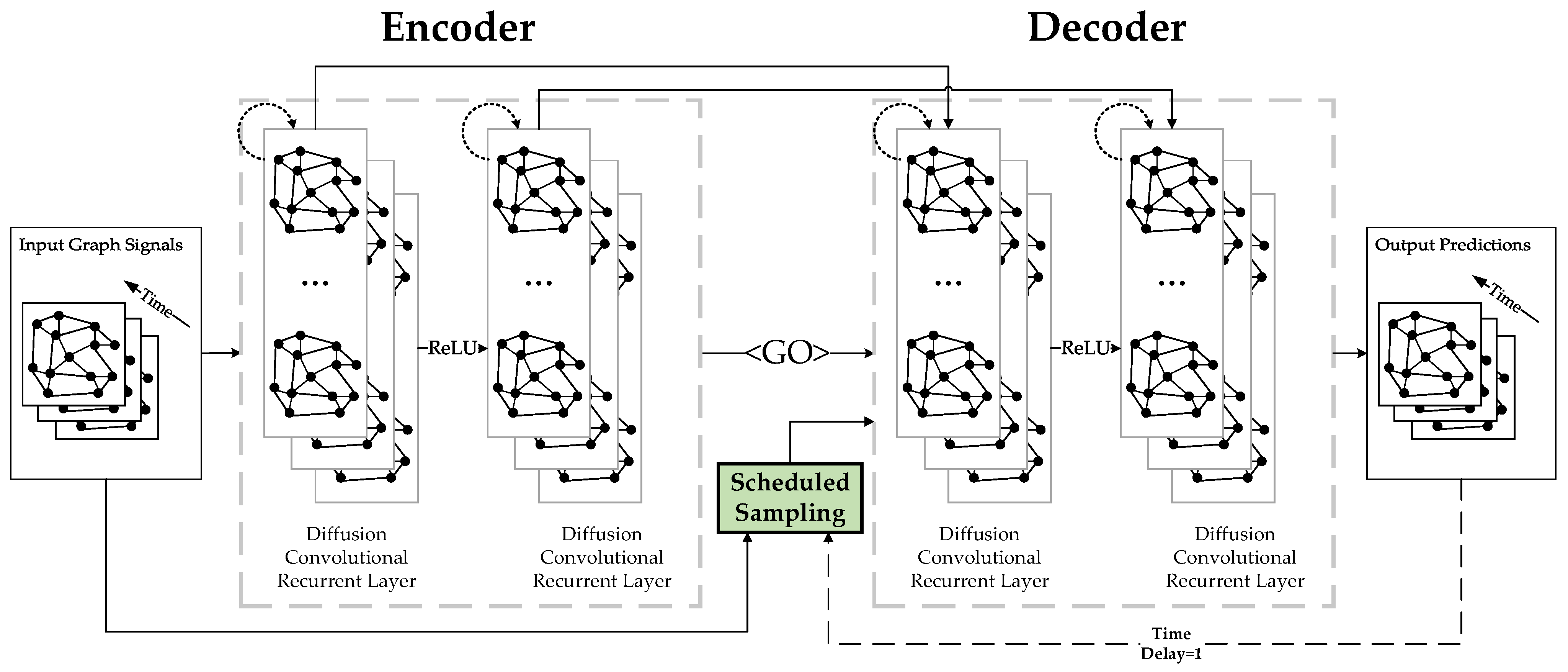
Sequence to Sequence (Seq2Seq) [38] model is a type of neural network architecture that is commonly used for sequence prediction or generation. The fundamental idea of the Seq2Seq models is to use an encoder–decoder architecture. In the model, the encoder network maps an input sequence into a fixed-length vector representation and the decoder network generates the output sequence based on the vector representation. The DCRNN adopts the Seq2Seq model architecture with both encoder and decoder implemented by the DCGRU, which enables the network to effectively perform multi-step prediction tasks with temporal dependencies.

During the training phase, the encoder of the Seq2Seq architecture takes the historical time series as input and generates final states, which are then used to initialize the decoder. The decoder is responsible for generating predictions based on the ground truth values that are previously observed. During the testing phase, the model uses its own predictions as inputs instead of the ground truth values. However, the discrepancy between the input distributions during training and testing can decline the model performance. In order to mitigate the potential degradation of performance caused by the discrepancy between input distributions, the DCRNN integrates Scheduled Sampling [35] into the model. Specifically, the DCRNN generates predictions that simultaneously capture the temporal dependencies of the multi-source inputs and the spatial dependencies of the topological features. When training, the model puts ground truth inputs into the decoder. During testing, the model feeds the predictions generated by the decoder as inputs to the next time step. Scheduled Sampling balances the use of the ground truth values and the model-generated inputs during training, which can make the model more robust when testing. A pseudo-code is presented in Algorithm 1

Algorithm 1: DCRNN

Input: historical graph signals ${(X}^{\left(t-\delta +1\right)},\dots ,X^{\left(t\right)}$) and graph $G=(V,E,M)$. Output: DCRNN model and future graph signals $\left(X^{\left(t+1\right)},\dots ,X^{\left(t+o\right)}\right)$. 1. Define the topology of the bus transit network using a weighted graph $G=(V,E,M)$. 2. Represent the volume of transit card transactions on $G$ as a graph signal $X\in {ℝ}^{N\times I}$, where $N$ is the total number of bus lines and $I$ is the number of features of each vertex. 3. Define a function $\xi \left(\cdot \right)$ that maps $\delta$ historical graph signals to $o$ future graph signals, given graph $G:\left(X^{\left(t-\delta +1\right)},\dots ,X^{\left(t\right)};G\right)\stackrel{\xi \left(\cdot \right)}{\to }\left(X^{\left(t+1\right)},\dots ,X^{\left(t+o\right)}\right)$. 4. Integrate diffusion convolution into a recurrent neural network to capture the spatiotemporal relationships:  (a) Define a DCRNN structure.  (b) Use a diffusion convolutional filter with a learnable parameter $\theta$, the maximum number of diffusion steps $Y,$ and restart probability $p$ to control the degree of diffusion.  (c) Normalize the graph signals based on the adjacency matrix $M$ in $G$.  (d) Apply the GDC layer on each feature of the graph signal $X$ to obtain the output graph signal.  (e) Combine GDC, RNN, and Seq2Seq to achieve multi-step input and multi-step output prediction. 5. Train the model by maximizing the likelihood of generating the target future time series using backpropagation through time.

With the spatial and temporal modeling structures described above, a DCRNN is built as shown in Figure 2. The network is trained by maximizing the likelihood of generating the target future time series using backpropagation through time. With the incorporation of both spatial and temporal dependencies along time series, the DCRNN captures the complex spatiotemporal patterns in various forecasting tasks. As a result, the DCRNN is applied for bus passenger flow prediction in a bus network.

3. Study Area and Data Processing

3.1. Temporal Patterns of Daily Ridership

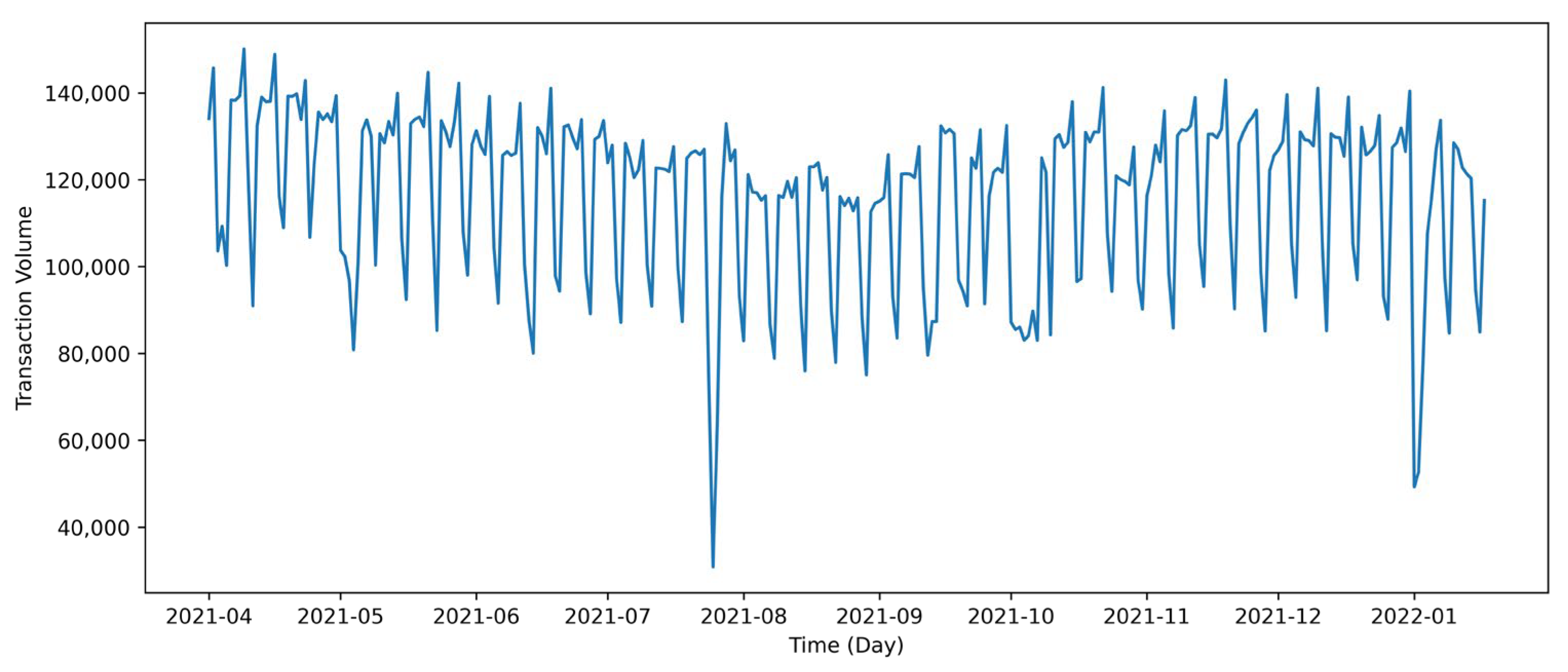
In this study, we focus on the bus network in Jiading District of Shanghai. The IC card transaction data from April 2021 to January 2022 are incorporated into this study. The data include the name of the bus line, the time of transaction, the bus fare, and the identification number of the IC card. The total daily ridership during the 10-month study period is presented in Figure 3. In the figure, we can find that the daily ridership roughly ranges from 80,000 (on weekends and holidays) to 14,000 (on workdays). Except for the great drop in bus ridership in late July 2021 caused by the landfall of Typhoon In-Fa, it presents a high regularity with recurrent patterns across the study period. The diurnal travel demand shares similar rhythms every week.

To process the data for bus passenger flow prediction, the following steps are conducted. First, we aggregate the individual transaction records with a 15-min granularity and interpolate the missing or anomalous values. Second, considering the characteristics of bus schedules that normally operate the buses during the daytime with fixed first and last bus trip requirements, we retain the hours from 6:00 to 22:00 each day for prediction. Next, to construct the data into a specific format, a matrix with the size of $m\times n$ is developed. In the matrix, the rows represent the dimension of time with a 15-min time interval for each row. The values in the y-axis refer to the total number of passengers boarding the bus on the corresponding bus line at each time interval.

3.2. Spatial Distribution and Construction of Graph for Bus Network

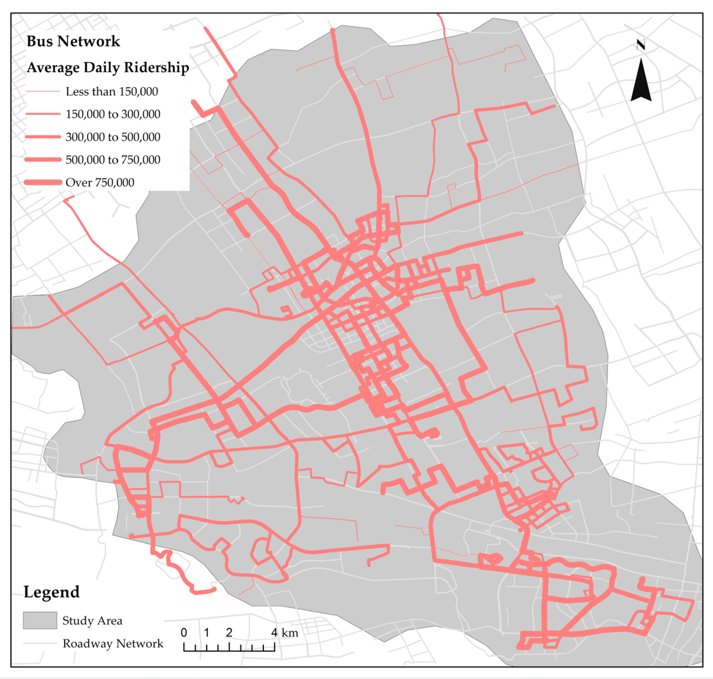
To study the spatial relationships among the bus lines, 59 bus routes are selected for this work with $n=59$. The layout of the bus network is shown in Figure 4. The figure also shows the average daily ridership of each bus line. It presents a clear pattern of spatial correlation of the bus ridership in different bus lines. The ridership in a bus line crossing or overlapping other high-demand bus lines is normally great as well, while the bus lines with low ridership cluster around the other low-ridership bus lines.

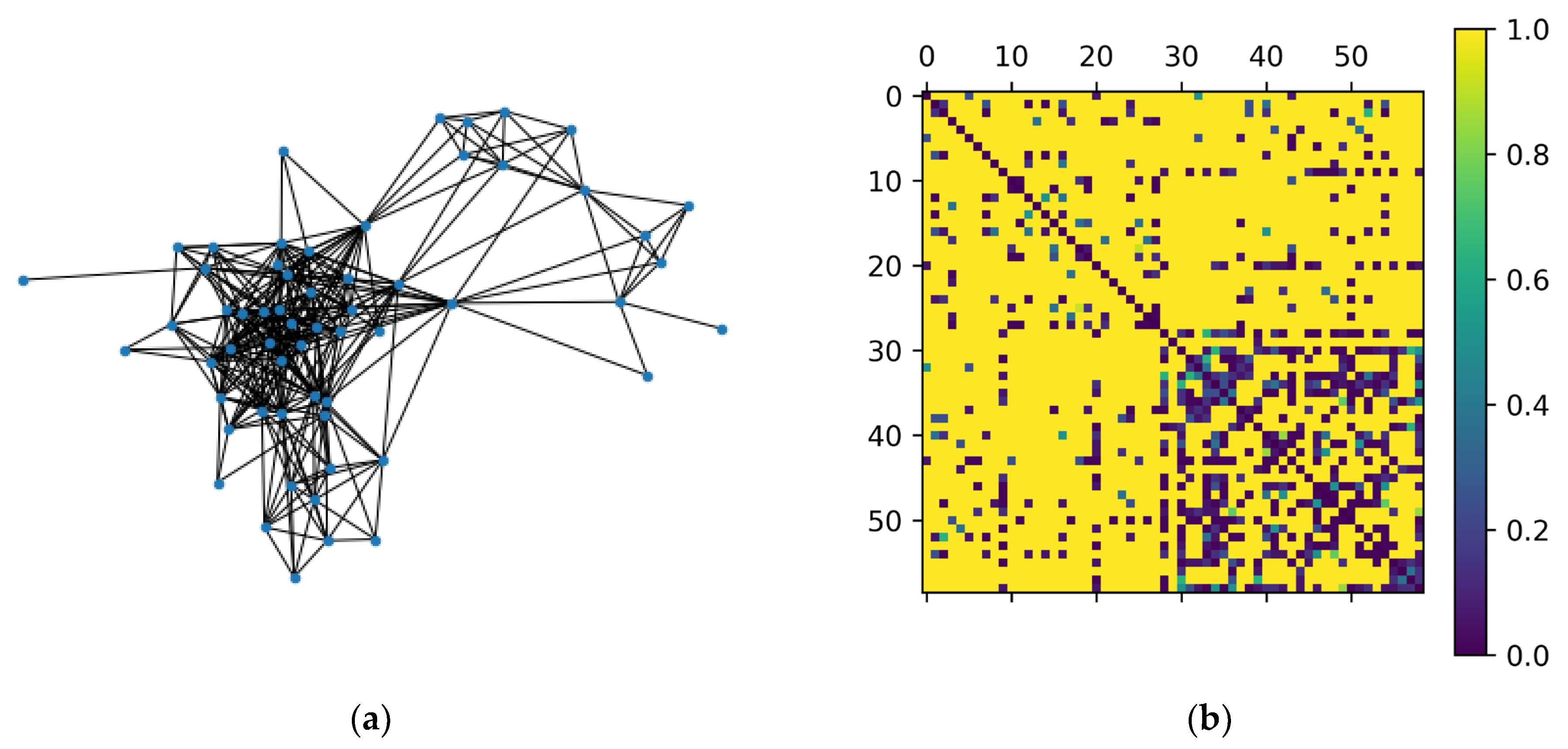
To better capture the spatial patterns in bus demand evolution, the topological structure of the bus network is mapped, where a vertex represents a bus line, shown in Figure 5a. The weights of the edges are determined by the number of shared bus stops between the bus lines. We use a Standard Gaussian Kernel to build the adjacency matrix. A transformation is also performed on the numerical values based on multiple experiments:

$$M_{ij}=\left\{\begin{array}{l}\frac{2}{\exp \left(-\mathrm{s}\mathrm{i}\mathrm{m}\mathrm{i}\mathrm{l}\mathrm{a}\mathrm{r}\mathrm{i}\mathrm{t}\mathrm{y}{\left(v_i,v_j\right)}^2/{\sigma }^2\right)}-1 i\ne j\\ 0 \hspace{1em}\hspace{1em}\hspace{1em}\hspace{1em}\hspace{1em}\hspace{1em}\hspace{1em}\hspace{1em}\hspace{1em}i=j\end{array}\right.$$

(14)

where $M_{ij}$ represents the weight of the edge between bus line $v_i$ and bus line $v_j$; $\mathrm{s}\mathrm{i}\mathrm{m}\mathrm{i}\mathrm{l}\mathrm{a}\mathrm{r}\mathrm{i}\mathrm{t}\mathrm{y}\left(v_i,v_j\right)$ denotes the common stops of line $v_i$ and line $v_j$; and $\sigma$ is the standard deviation of stops. The adjacency matrix is visualized in Figure 5b.

4. Results and Discussion

4.1. Metrics for Modeling Evaluation

We normalize the input data to ensure that each feature contributes equally to the analysis. The dataset is split into three subsets for training, testing, and validation, respectively. The DCRNN models are coded in Python 3.8 based on the PyTorch deep learning framework and are then loaded in an Ubuntu 20.04 server equipped with one Nvidia RTX 4090 and two Nvidia RTX 3090 graphics cards for training and tuning.

In the proposed models, ReLU is employed as the activation function, while the loss function is defined based on the mean square error. We use Adam optimizer to train the weights of the neural network with Early-Stopping technique to enhance the effectiveness of training.

After training, the models are tested and evaluated using the following statistical indices, which are the Mean Absolute Percentage Error (MAPE) expressed in Equation (15), t the Mean Absolute Error (MAE) expressed in Equation (16), and the Root Mean Square Error (RMSE) expressed in Equation (17). The MAPE is used to evaluate the accuracy of the model prediction in percentage, while MAE and RMSE measure the difference between the predicted and actual values [39].

$$\mathrm{M}\mathrm{A}\mathrm{P}\mathrm{E}=\frac{1}{n}\sum _{i=1}^n\left|\frac{{\eta }_i-{\mu }_i}{{\eta }_i}\right|\times 100\%$$

(15)

$$\mathrm{M}\mathrm{A}\mathrm{E}=\frac{1}{n}\sum _{i=1}^n\left|{\eta }_i-{\mu }_i\right|$$

(16)

$$\mathrm{R}\mathrm{M}\mathrm{S}\mathrm{E}=\sqrt{\frac{1}{n}\sum _{i=1}^n{\left({\eta }_i-{\mu }_i\right)}^2}$$

(17)

where ${\eta }_i$ and ${\mu }_i$ denote the actual ground truth values and the predicted values of the i-th data point, respectively; $n$ is the number of data points; and $v$ is the mean of the actual values.

4.2. Modeling Results with Different Hyperparameters

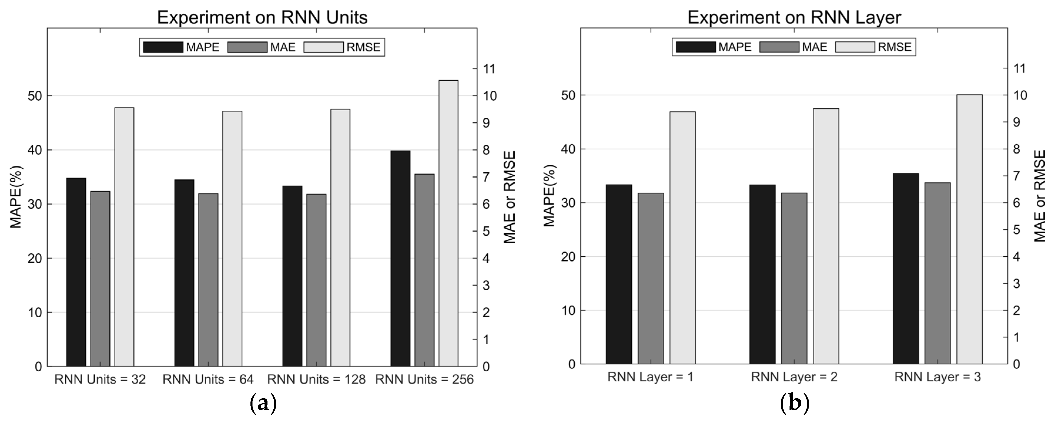
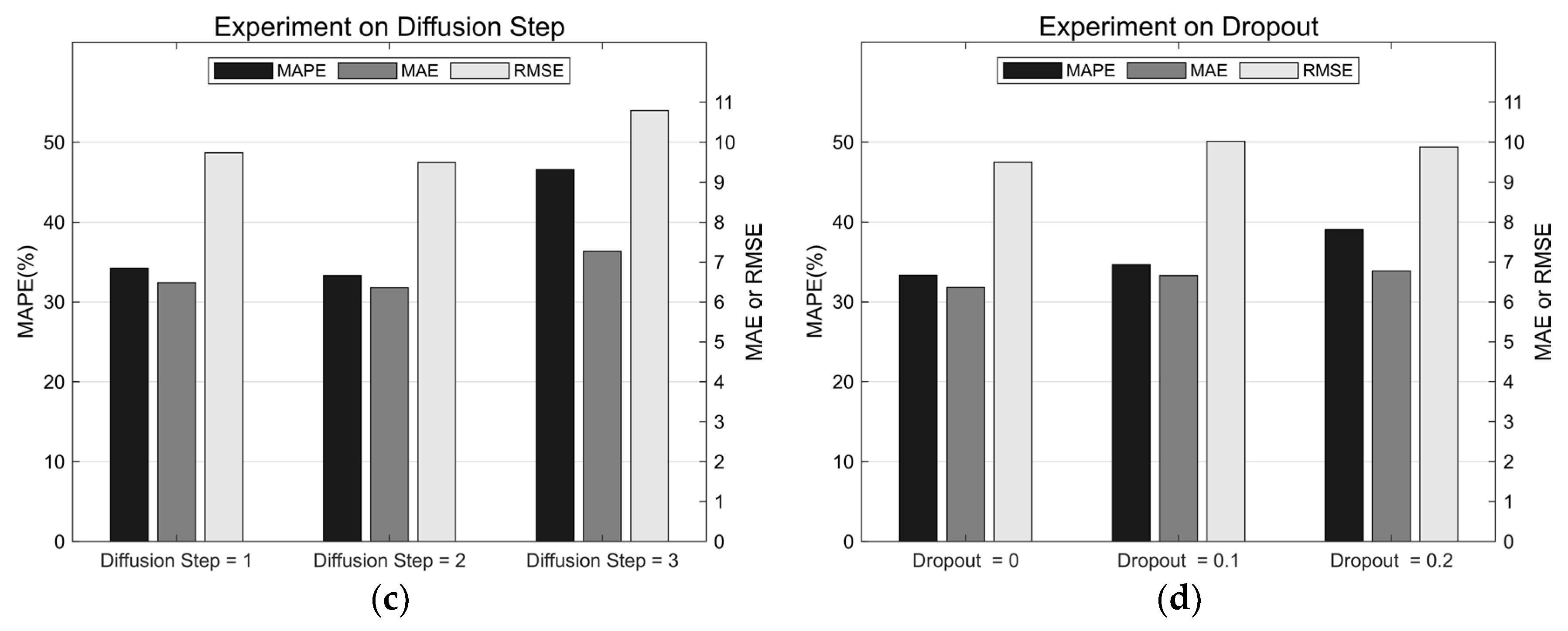
The hyper-parameters are determined based on the performance of the model on the validated dataset. The results of four different sets of experiments—RNN hidden units, RNN layers, diffusion steps, and dropout—are presented in Table 1 and Figure 6. Specifically, in each set, we focus on one of the four key hyperparameters:

(1)

The number of hidden units in each layer: the RNN units determine the model’s capacity and representational power, where a greater number of units result in a more complex model but also increase the risk of overfitting.

(2)

The number of layers in the model: The RNN layers also affect the complexity and learning capability of the model. Deeper layers make the modeling structure more sophisticated, but can also lead to potential issues such as gradient vanishing and/or exploding.

(3)

The diffusion steps of the graph convolutional filter: The diffusion steps affect the model’s ability to capture spatial information. A larger number of steps enable the model to better capture the relationships between the vertices in a network that are distant from each other. However, it may also lead to the overfitting of the model and make it more demanding in computation.

(4)

The dropout parameter of the model: the dropout parameter helps the model mitigate the overfitting issue by randomly dropping a certain proportion of neurons during the training process.

Table 1. Four sets of experiments on hyperparameters.

Case	Baseline Parameter	Hyper Parameter	MAPE	MAE	RMSE	Number of Parameters
1	RNN Layers = 2, Diffusion steps = 2, Dropout = 0	RNN Units = 32	34.80%	6.47	9.56	94,017
		RNN Units = 64	34.47%	6.38	9.43	372,353
		RNN Units = 128	33.32%	6.36	9.50	1,481,985
		RNN Units = 256	39.81%	7.10	10.56	5,913,089
2	RNN Units = 128, Diffusion steps = 2, Dropout = 0	RNN Layers = 1	33.36%	6.36	9.38	498,177
		RNN Layers = 2	33.32%	6.36	9.50	1,481,985
		RNN Layers = 3	35.46%	6.74	10.01	2,465,793
3	RNN Units = 128, RNN Layers = 2, Dropout = 0	Diffusion Steps = 1	34.24%	6.49	9.74	889,857
		Diffusion Steps = 2	33.32%	6.36	9.50	1,481,985
		Diffusion Steps = 3	46.58%	7.27	10.79	2,074,113
4	RNN Units = 128, RNN Layers = 2, Diffusion steps = 2	Dropout = 0	33.32%	6.36	9.50	1,481,985
		Dropout = 0.1	34.67%	6.66	10.02	1,481,985
		Dropout = 0.2	39.08%	6.77	9.88	1,481,985

Table 1. Four sets of experiments on hyperparameters.

Case	Baseline Parameter	Hyper Parameter	MAPE	MAE	RMSE	Number of Parameters
1	RNN Layers = 2, Diffusion steps = 2, Dropout = 0	RNN Units = 32	34.80%	6.47	9.56	94,017
		RNN Units = 64	34.47%	6.38	9.43	372,353
		RNN Units = 128	33.32%	6.36	9.50	1,481,985
		RNN Units = 256	39.81%	7.10	10.56	5,913,089
2	RNN Units = 128, Diffusion steps = 2, Dropout = 0	RNN Layers = 1	33.36%	6.36	9.38	498,177
		RNN Layers = 2	33.32%	6.36	9.50	1,481,985
		RNN Layers = 3	35.46%	6.74	10.01	2,465,793
3	RNN Units = 128, RNN Layers = 2, Dropout = 0	Diffusion Steps = 1	34.24%	6.49	9.74	889,857
		Diffusion Steps = 2	33.32%	6.36	9.50	1,481,985
		Diffusion Steps = 3	46.58%	7.27	10.79	2,074,113
4	RNN Units = 128, RNN Layers = 2, Diffusion steps = 2	Dropout = 0	33.32%	6.36	9.50	1,481,985
		Dropout = 0.1	34.67%	6.66	10.02	1,481,985
		Dropout = 0.2	39.08%	6.77	9.88	1,481,985

The detailed results with four different hyperparameters on the model are listed in Table 1. In case 1, with the increasing number of hidden units per layer in the neural network, the accuracy of the model gradually improves. However, after reaching a certain point, with 256 hidden units, the model accuracy suddenly decreases. Similarly, in case 2, the model accuracy presents a similar pattern. There is not much difference in accuracy between a one-layer and a two-layer network. However, when the number of layers increases to three, the MAPE increases from 33.3% to 35.5%, and the other performance metrics also show significant degradation.

In case 1 and case 2, we can find that the increase in the number of units and layers does not necessarily lead to a monotonic improvement of network performance. The increased depth of the network may bring the gradient to vanish or explode, resulting in unstable updates of the gradient during the training process. Second, with more units and layers, the number of trainable parameters largely increases, potentially leading to overfitting if the volume of training data is limited. It thus reduces the generalization ability of the models. In addition, a more complex network structure prolongs the training time with greater computational costs.

In case 3, we test the impacts of different diffusion steps. The diffusion step can be interpreted as proximity to the size of the receptive field. With larger receptive fields, the model captures broader spatial dependencies. However, the complexity of the model also increases. With diffusion steps increasing from one to three, the predicted MAPE decreases from 34% to 33%, but then sharply rises to 47%. It indicates that with greater diffusion steps, the weights of the graph become more evenly distributed. Therefore, the neural network learns less effective knowledge. This also suggests that the number of passengers in a bus line is more similar to the numbers in the closely related bus lines. The distant lines may have little impact, which also confirms the effectiveness of the incorporation of diffusion convolution. With more diffusion steps, the total number of trainable parameters significantly increases, resulting in a longer training time. In case 4, it shows that different settings of dropout parameters do not lead to a significant improvement in performance.

In summary, to ensure the accuracy of the model with a greater sensitivity on smaller prediction values, we choose the group of hyperparameters with the smallest MAPE. The chosen set of hyperparameters is: {number of hidden units in each layer = 128, number of layers = 2, diffusion steps = 2, dropout = 0}.

4.3. Comparison with Alternative Models

To demonstrate the advantages of the proposed DCRNN model, we will compare it with the other five classic models. The comparative models include two classic RNN models, LSTM and GRU [40], and three statistical models—the static model, the historical average (HA) model, and the vector auto-regression (VAR) model.

Specifically, the static model simply assumes that $X^{t+1}=X^t$, meaning the data for the next time period is the same as the previous cycle. The HA captures the evolution of bus travel demand as a seasonal process. It predicts future values by using a weighted average from the past seasons. In this work, we use a period of one week and aggregate the data from previous weeks for predictions. For instance, to predict the bus passenger flow on this Friday, we take the average bus passenger flow from past Fridays. As the HA method does not rely on short-term data, its performance remains stable in the presence of slight disturbances and noise. The VAR models the relationship between multiple time series variables. It has been widely used in transportation research to predict bus passenger flows by considering the interdependencies among multiple transit-related variables. The lag value is set to three in this paper.

Due to the fact that LSTM and GRU are both deep neural network models, we also performed hyperparameter selection for fine-tuning these two models. As shown in

Table 2. Selection of hyperparameters on LSTM and GRU.

Model	Baseline Parameter	Hyper Parameter	MAPE	MAE	RMSE
LSTM	RNN Layer = 2 Dropout = 0.2	RNN Units = 32	38.93%	6.34	9.49
		RNN Units = 64	40.93%	6.48	9.65
		RNN Units = 128	39.23%	6.29	9.43
		RNN Units = 256	38.06%	6.43	9.76
GRU	RNN Layer = 2 Dropout = 0.2	RNN Units = 32	38.90%	6.33	9.45
		RNN Units = 64	44.23%	6.64	9.73
		RNN Units = 128	39.90%	6.37	9.54
		RNN Units = 256	38.65%	6.56	10.03

, the hyperparameters were chosen based on the same criteria as for DCRNN. We select the set of hyperparameters with the smallest MAPE. For both models, the set of hyperparameters is {the number of units of each RNN layer = 256, the number of network layers = 2, dropout = 0.2}.

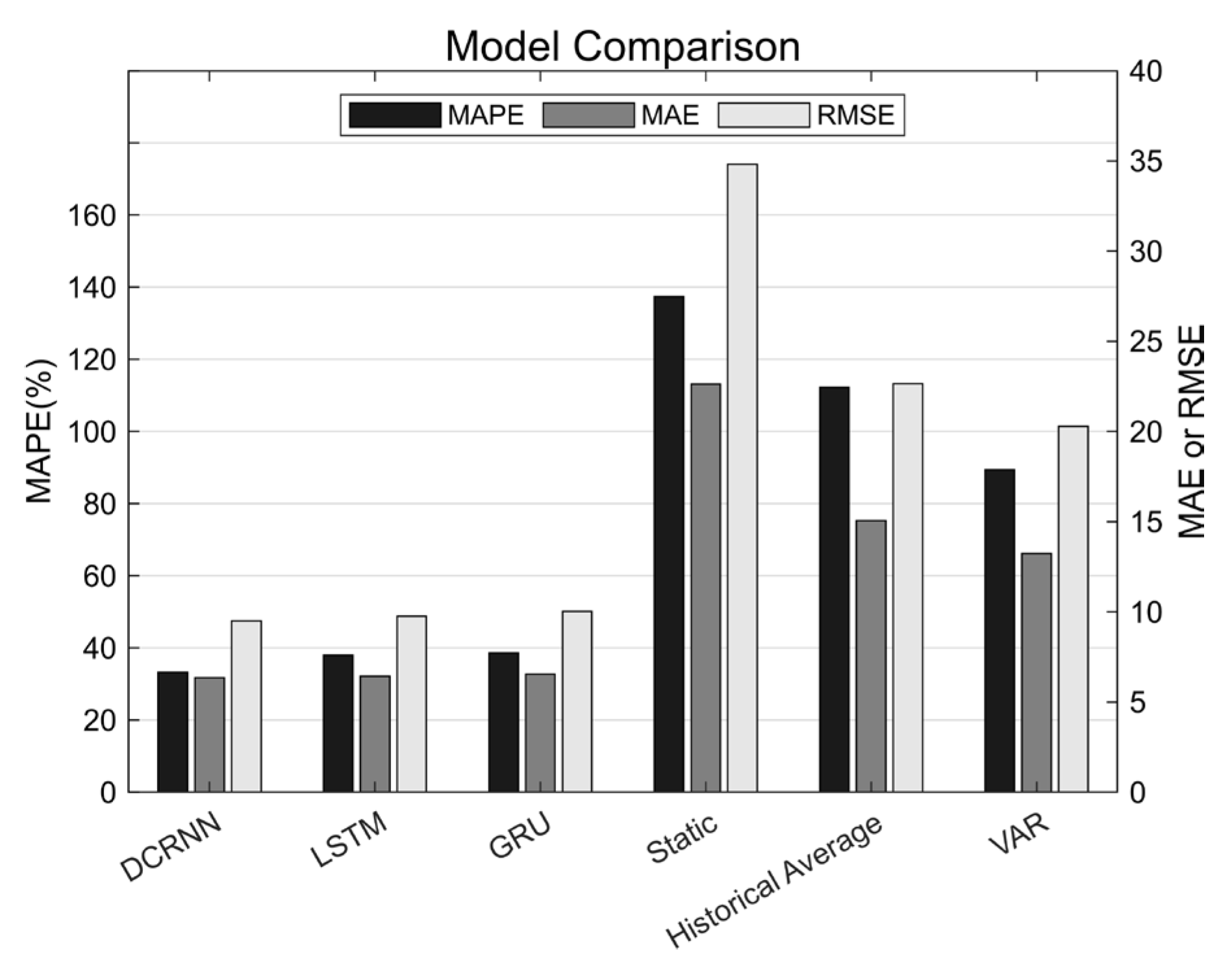
The datasets for training and prediction data are kept consistent for all models. The model comparison results are given in Table 3 and visualized in Figure 7. It is evident that all three neural network models outperform the other three traditional models. Compared with the LSTM and GRU, the DCRNN presents a significant advantage of about 4–5% improvement in terms of MAPE with a comparable performance of MAE and RMSE.

Table 3. Model comparison results.

Model	MAPE	MAE	RMSE
DCRNN	33.32%	6.36	9.50
LSTM	38.06%	6.43	9.76
GRU	38.65%	6.56	10.03
Static	137.45%	22.64	34.81
Historical Average	112.32%	15.07	22.66
VAR	89.48%	13.25	20.3

Table 3. Model comparison results.

Model	MAPE	MAE	RMSE
DCRNN	33.32%	6.36	9.50
LSTM	38.06%	6.43	9.76
GRU	38.65%	6.56	10.03
Static	137.45%	22.64	34.81
Historical Average	112.32%	15.07	22.66
VAR	89.48%	13.25	20.3

The similar values of MAE or RMSE indicate that the average difference between the absolute or squared values of the prediction errors is not significant, which means that the model has a balanced capability to reduce the size of prediction errors. Nonetheless, if the MAPE metric is smaller, it means that the model’s prediction capability is more balanced and robust for very small and very large values. This indicates that the DCRNN has a more consistent performance in bus passenger flow forecasting with smaller prediction errors for the case of smaller predicted values, making it more reliable than the classic LSTM and GRU models.

4.4. Discussion

An accurate prediction of bus passenger flow is significantly important for the improvement of transit service efficiency by optimizing the allocation of service resources. For real-time bus operation, short-term passenger flow prediction is needed for bus operators to better understand the changes in passenger flow during different time periods, as well as the distribution of passenger flow among different bus routes. Thus, they can dispatch the vehicles and crews to match the bus passengers’ travel demand more precisely, avoiding service hazards such as overcrowding/overloading, long waiting times, etc., thereby improving the passengers’ experience.

The challenge of optimizing the real-time dispatching strategies of bus operations lies in how to better re-allocate the limited bus vehicles and crews from low-demand bus lines to high-demand bus lines. In other words, to support the high-demand bus routes, it is crucial to ensure the basic level of service of the low-demand lines, meaning that the passengers in low-demand routes should not be significantly affected. Therefore, to relocate the bus resources to high-demand routes, the prediction of travel demand in low-demand routes is essential for maintaining the level of bus service.

Since neural networks capture more non-linear features compared with traditional machine learning models [16], in this work, we can find that the LSTM, GRU, and DCRNN models all significantly outperform the other three models, i.e., the static, HA, and VAR. Compared with the LSTM and the GRU models, the DCRNN adopted in this work that incorporates spatial interactions between bus lines has a lower value of MAPE. This indicates that the model is more accurate and sensitive in forecasting the travel demand in low-demand bus routes, which can provide better support for real-time inter-line operation for bus operators with more precise prediction in the ridership of low-demand bus lines. Although LSTM and GRU are widely implemented for time series prediction, they are not able to capture the spatial dependencies among different routes in the bus network. DCRNN, however, leverages diffusion convolution to capture spatiotemporal dependencies, thereby achieving more accurate predictions of bus passenger flows. What has to be noted is that the DCRNN model has a more complex architecture that requires a large amount of data for training. The training time spent for DCRNN is quadruple the time spent for LSTM and GRU. Nonetheless, once the DCRNN model is well trained, the running speed of the model for prediction tasks is not inferior to other classic RNN models.

5. Conclusions

This article utilizes an end-to-end deep learning framework for the short-term forecasting of the passenger flows of each bus line in a bus transit network. A graph-based DCRNN structure is developed to extract and adaptively learn the relationships between bus lines in the network since bus passengers interchange between these lines. As the bus networks are not grid-like, we adopt graph convolution to learn the topological features of the network. The model considers the impacts of distance decay in a series of spatially correlated vertices in a graph by introducing the diffusion convolution process. The RNN and Seq2Seq structures incorporated in the model can also capture the time-series information. The proposed DCRNN model is performed using 10-month consecutive transactional data from the bus services in Jiading of Shanghai, which shows greater accuracy, especially in predicting low-demand bus lines, compared with classic RNN models.

It must be noted that there are also limitations to this study. First, the data adopted in this work only include transaction records with transit IC cards and Quick Response (QR) code scanning. The information about passengers paying in cash is not included. Although the share of cash-paying passengers is relatively low, the lack of such information may also impact the accuracy of the model. In addition, the passengers do not swap their IC cards or scan the QR codes again when alighting. Therefore, in this work, the bus passenger flow means the number of passengers boarding a bus line but not in a specific bus vehicle. To get the accurate passenger flow in each bus vehicle, additional work needs to be conducted for alighting stop inference.

For future research, external information such as weather information can be considered to enrich the inputs of the model. Furthermore, the prediction of the number of passengers boarding at each bus stop and the passenger flow in each bus vehicle should also be investigated with more detailed data at the stop level.

References

1. Alomari, A.H.; Khedaywi, T.S.; Jadah, A.A.; Marian, A.R.O. Evaluation of Public Transport among University Commuters in Rural Areas. Sustainability 2023, 15, 312. [Google Scholar] [CrossRef]
2. Anderson, M.L. Subways, Strikes, and Slowdowns: The Impacts of Public Transit on Traffic Congestion. Am. Econ. Rev. 2014, 104, 2763–2796. [Google Scholar] [CrossRef] [Green Version]
3. Nagaraj, N.; Gururaj, H.L.; Swathi, B.H.; Hu, Y.-C. Passenger Flow Prediction in Bus Transportation System Using Deep Learning. Multimed. Tools Appl. 2022, 81, 12519–12542. [Google Scholar] [CrossRef]
4. Tirachini, A.; Hensher, D.A.; Rose, J.M. Crowding in Public Transport Systems: Effects on Users, Operation and Implications for the Estimation of Demand. Transp. Res. Part A Policy Pract. 2013, 53, 36–52. [Google Scholar] [CrossRef]
5. Liu, C.; Shen, Q. An Empirical Analysis of the Influence of Urban Form on Household Travel and Energy Consumption. Comput. Environ. Urban Syst. 2011, 35, 347–357. [Google Scholar] [CrossRef]
6. Luo, D.; Zhao, D.; Ke, Q.; You, X.; Liu, L.; Zhang, D.; Ma, H.; Zuo, X. Fine-Grained Service-Level Passenger Flow Prediction for Bus Transit Systems Based on Multitask Deep Learning. IEEE Trans. Intell. Transp. Syst. 2021, 22, 7184–7199. [Google Scholar] [CrossRef]
7. Ahmed, M.S.; Cook, A.R. Analysis of Freeway Traffic Time-Series Data by Using Box-Jenkins Techniques; Transportation Research Record; Transportation Research Board: Washington, DC, USA, 1979. [Google Scholar]
8. Williams, B.M.; Durvasula, P.K.; Brown, D.E. Urban Freeway Traffic Flow Prediction: Application of Seasonal Autoregressive Integrated Moving Average and Exponential Smoothing Models. Transp. Res. Rec. 1998, 1644, 132–141. [Google Scholar] [CrossRef]
9. Williams, B.M.; Hoel, L.A. Modeling and Forecasting Vehicular Traffic Flow as a Seasonal ARIMA Process: Theoretical Basis and Empirical Results. J. Transp. Eng. 2003, 129, 664–672. [Google Scholar] [CrossRef] [Green Version]
10. Li, X.; Pan, G.; Wu, Z.; Qi, G.; Li, S.; Zhang, D.; Zhang, W.; Wang, Z. Prediction of Urban Human Mobility Using Large-Scale Taxi Traces and Its Applications. Front. Comput. Sci. 2012, 6, 111–121. [Google Scholar]
11. Jiao, P.; Li, R.; Sun, T.; Hou, Z.; Ibrahim, A. Three Revised Kalman Filtering Models for Short-Term Rail Transit Passenger Flow Prediction. Math. Probl. Eng. 2016, 2016, e9717582. [Google Scholar] [CrossRef] [Green Version]
12. Su, H.; Zhang, L.; Yu, S. Short-Term Traffic Flow Prediction Based on Incremental Support Vector Regression. In Proceedings of the Third International Conference on Natural Computation (ICNC 2007), Haikou, China, 24–27 August 2007; Volume 1, pp. 640–645. [Google Scholar]
13. Cheng, S.; Lu, F.; Peng, P.; Wu, S. Short-Term Traffic Forecasting: An Adaptive ST-KNN Model That Considers Spatial Heterogeneity. Comput. Environ. Urban Syst. 2018, 71, 186–198. [Google Scholar] [CrossRef]
14. Toqué, F.; Khouadjia, M.; Come, E.; Trepanier, M.; Oukhellou, L. Short & Long Term Forecasting of Multimodal Transport Passenger Flows with Machine Learning Methods. In Proceedings of the 2017 IEEE 20th International Conference on Intelligent Transportation Systems (ITSC), Yokohama, Japan, 16–19 October 2017; pp. 560–566. [Google Scholar]
15. Li, Y.; Ma, C. Short-Time Bus Route Passenger Flow Prediction Based on a Secondary Decomposition Integration Method. J. Transp. Eng. Part A Syst. 2023, 149, 04022132. [Google Scholar] [CrossRef]
16. Nguyen, H.; Kieu, L.-M.; Wen, T.; Cai, C. Deep Learning Methods in Transportation Domain: A Review. IET Intell. Transp. Syst. 2018, 12, 998–1004. [Google Scholar] [CrossRef]
17. Gang, X.; Kang, W.; Wang, F.; Zhu, F.; Lv, Y.; Dong, X.; Riekki, J.; Pirttikangas, S. Continuous Travel Time Prediction for Transit Signal Priority Based on a Deep Network. In Proceedings of the 2015 IEEE 18th International Conference on Intelligent Transportation Systems, Gran Canaria, Spain, 15–18 September 2015; pp. 523–528. [Google Scholar]
18. Ma, X.; Tao, Z.; Wang, Y.; Yu, H.; Wang, Y. Long Short-Term Memory Neural Network for Traffic Speed Prediction Using Remote Microwave Sensor Data. Transp. Res. Part C Emerg. Technol. 2015, 54, 187–197. [Google Scholar] [CrossRef]
19. Duan, Y.; Lv, Y.; Wang, F.-Y. Travel Time Prediction with LSTM Neural Network. In Proceedings of the 2016 IEEE 19th International Conference on Intelligent Transportation Systems (ITSC), Rio de Janeiro, Brazil, 1–4 November 2016; pp. 1053–1058. [Google Scholar]
20. Huang, W.; Song, G.; Hong, H.; Xie, K. Deep Architecture for Traffic Flow Prediction: Deep Belief Networks With Multitask Learning. IEEE Trans. Intell. Transp. Syst. 2014, 15, 2191–2201. [Google Scholar] [CrossRef]
21. Ke, J.; Zheng, H.; Yang, H.; Chen, X. (Michael) Short-Term Forecasting of Passenger Demand under on-Demand Ride Services: A Spatio-Temporal Deep Learning Approach. Transp. Res. Part C Emerg. Technol. 2017, 85, 591–608. [Google Scholar] [CrossRef] [Green Version]
22. Perez, L.; Wang, J. The Effectiveness of Data Augmentation in Image Classification Using Deep Learning. arXiv 2017, arXiv:1712.04621. [Google Scholar] [CrossRef]
23. Young, T.; Hazarika, D.; Poria, S.; Cambria, E. Recent Trends in Deep Learning Based Natural Language Processing. IEEE Comput. Intell. Mag. 2018, 13, 55–75. [Google Scholar] [CrossRef]
24. Schlichtkrull, M.; Kipf, T.N.; Bloem, P.; van den Berg, R.; Titov, I.; Welling, M. Modeling Relational Data with Graph Convolutional Networks. In The Semantic Web, Proceedings of the 15th International Conference, ESWC 2018, Heraklion, Crete, Greece, 3–7 June 2018; Gangemi, A., Navigli, R., Vidal, M.-E., Hitzler, P., Troncy, R., Hollink, L., Tordai, A., Alam, M., Eds.; Springer International Publishing: Cham, Switzerland, 2018; pp. 593–607. [Google Scholar]
25. Yu, B.; Yin, H.; Zhu, Z. Spatio-Temporal Graph Convolutional Networks: A Deep Learning Framework for Traffic Forecasting. In Proceedings of the Twenty-Seventh International Joint Conference on Artificial Intelligence, Stockholm, Sweden, 13–19 July 2018; pp. 3634–3640. [Google Scholar]
26. Polson, N.G.; Sokolov, V.O. Deep Learning for Short-Term Traffic Flow Prediction. Transp. Res. Part C Emerg. Technol. 2017, 79, 1–17. [Google Scholar] [CrossRef] [Green Version]
27. Liu, Y.; Liu, Z.; Jia, R. DeepPF: A Deep Learning Based Architecture for Metro Passenger Flow Prediction. Transp. Res. Part C Emerg. Technol. 2019, 101, 18–34. [Google Scholar] [CrossRef]
28. Ren, Y.; Chen, H.; Han, Y.; Cheng, T.; Zhang, Y.; Chen, G. A Hybrid Integrated Deep Learning Model for the Prediction of Citywide Spatio-Temporal Flow Volumes. Int. J. Geogr. Inf. Sci. 2020, 34, 802–823. [Google Scholar] [CrossRef]
29. Zhao, T.; Huang, Z.; Tu, W.; He, B.; Cao, R.; Cao, J.; Li, M. Coupling Graph Deep Learning and Spatial-Temporal Influence of Built Environment for Short-Term Bus Travel Demand Prediction. Comput. Environ. Urban Syst. 2022, 94, 101776. [Google Scholar] [CrossRef]
30. Chen, T.; Fang, J.; Xu, M.; Tong, Y.; Chen, W. Prediction of Public Bus Passenger Flow Using Spatial–Temporal Hybrid Model of Deep Learning. J. Transp. Eng. Part A Syst. 2022, 148, 04022007. [Google Scholar] [CrossRef]
31. Baghbani, A.; Bouguila, N.; Patterson, Z. Short-Term Passenger Flow Prediction Using a Bus Network Graph Convolutional Long Short-Term Memory Neural Network Model. Transp. Res. Rec. 2023, 2677, 1331–1340. [Google Scholar] [CrossRef]
32. Zhao, C.; Song, A.; Du, Y.; Yang, B. TrajGAT: A Map-Embedded Graph Attention Network for Real-Time Vehicle Trajectory Imputation of Roadside Perception. Transp. Res. Part C Emerg. Technol. 2022, 142, 103787. [Google Scholar] [CrossRef]
33. Atwood, J.; Towsley, D. Diffusion-Convolutional Neural Networks. In Proceedings of the Advances in Neural Information Processing Systems 29 (NIPS 2016), Barcelona, Spain, 5–10 December 2016; Curran Associates, Inc.: Sydney, Australia, 2016. [Google Scholar]
34. Gasteiger, J.; Weißenberger, S.; Günnemann, S. Diffusion Improves Graph Learning. In Proceedings of the Advances in Neural Information Processing Systems 32 (NeurIPS 2019), Vancouver, BC, Canada, 8–14 December 2019; Curran Associates, Inc.: Sydney, Australia, 2019. [Google Scholar]
35. Li, Y.; Yu, R.; Shahabi, C.; Liu, Y. Diffusion Convolutional Recurrent Neural Network: Data-Driven Traffic Forecasting. arXiv 2017, arXiv:1707.01926. [Google Scholar] [CrossRef]
36. Wang, H.-W.; Peng, Z.-R.; Wang, D.; Meng, Y.; Wu, T.; Sun, W.; Lu, Q.-C. Evaluation and Prediction of Transportation Resilience under Extreme Weather Events: A Diffusion Graph Convolutional Approach. Transp. Res. Part C Emerg. Technol. 2020, 115, 102619. [Google Scholar] [CrossRef]
37. Lin, L.; He, Z.; Peeta, S. Predicting Station-Level Hourly Demand in a Large-Scale Bike-Sharing Network: A Graph Convolutional Neural Network Approach. Transp. Res. Part C Emerg. Technol. 2018, 97, 258–276. [Google Scholar] [CrossRef] [Green Version]
38. Sutskever, I.; Vinyals, O.; Le, Q.V. Sequence to Sequence Learning with Neural Networks. In Proceedings of the Advances in Neural Information Processing Systems 27 (NIPS 2014), Montreal, QC, Canada, 8–13 December 2014; Curran Associates, Inc.: Sydney, Australia, 2014. [Google Scholar]
39. Zou, L.; Shu, S.; Lin, X.; Lin, K.; Zhu, J.; Li, L. Passenger Flow Prediction Using Smart Card Data from Connected Bus System Based on Interpretable XGBoost. Wirel. Commun. Mob. Comput. 2022, 2022, e5872225. [Google Scholar] [CrossRef]
40. Fu, R.; Zhang, Z.; Li, L. Using LSTM and GRU Neural Network Methods for Traffic Flow Prediction. In Proceedings of the 2016 31st Youth Academic Annual Conference of Chinese Association of Automation (YAC), Wuhan, China, 11–13 November 2016; pp. 324–328. [Google Scholar]
Figure 1. Illustration of the graph diffusion process with Y diffusion steps on a schematic graph.
Applsci 13 04910 g001
Figure 2. The architecture for the DCRNN for bus passenger flow prediction.
Applsci 13 04910 g002
Figure 3. Total daily ridership during the 10-month study period.
Applsci 13 04910 g003
Figure 4. Bus network and the distribution of average daily ridership at bus line level.
Applsci 13 04910 g004
Figure 5. (a) Graph visualization of 59 bus routes; (b) Visualization of adjacency matrix of the weighted graph.
Applsci 13 04910 g005
Figure 6. Comparison of the effect of each set of experiments on the model accuracy: (a) The impact of the number of hidden units; (b) The impact of the number of layers; (c) The impact of the diffusion steps; (d) The impact of dropout parameter.
Applsci 13 04910 g006aApplsci 13 04910 g006b
Figure 7. Model comparison between DCRNN and the baseline models.
Applsci 13 04910 g007