Abstract
This paper presents a study on controlling the out-of-water motion of amphibious multi-rotor UAVs using a cascade control method based on the Active Disturbance Rejection Control (ADRC) algorithm. The aim is to overcome the challenges of time-varying model parameters and complex external disturbances. The research involves developing an underwater dynamic model and analyzing hydrodynamic forces to calculate theoretical inertial hydrodynamic forces and simulate viscous hydrodynamic forces. This establishes the relationship between viscous hydrodynamic forces and exit velocity. A complete air dynamic model is then established, selecting model parameters based on the center of mass position of the amphibious vehicle to enable switching from water to air. To address control algorithm instability caused by changes in model parameters, position and attitude controllers are built using the ADRC algorithm. The control effects are compared with traditional PID and sliding mode controllers (SMC) to verify the effectiveness and superiority of the proposed cascade ADRC control strategy. Experimental results show that our controller has stronger anti-interference than traditional PID and SMC controllers and can overcome control instability caused by changes in model parameters. Our research highlights the importance of using ADRC-based controllers for amphibious multi-rotor UAVs to achieve robust and stable control.
1. Introduction
As a new type of robot, the amphibious multi-rotor UAV offers groundbreaking advantages over traditional UAVs and single-medium robots as they can operate continuously across multiple scenarios [1,2,3,4], making them a research hotspot in various countries [5,6,7,8]. However, they face the challenge of spanning different mediums and coping with the physical differences between water and air, as well as the interference of external factors such as water flow, wind, and waves. These changes can lead to variations in control model parameters. Traditional cross-medium control methods have low robustness and have difficulty in maintaining system stability when encountering complex environments, leading to cross-medium failure.
The cross-media technology of amphibious multi-rotor UAVs is a key area of research, and numerous scholars have made significant contributions to this field. In 2014, Drews et al. [9] proposed a two-stage approach to the spanning process, dividing it into airborne and underwater phases, and designed a corresponding dynamics model. They also established a simulation control system using a PD controller and verified the feasibility of their approach. In 2015, Neto et al. [10] proposed a switching approach to cross-media control, with separate robust controllers for air and underwater media. However, their method did not consider the variation in added mass and float, leading to limitations in seamless cross-media control.
In 2015, Yu Z et al. [11] designed a physical model of a symmetric cylindrical vehicle for an amphibious trans-media vehicle and investigated the underwater dynamics of the vehicle. In 2016, Siddall [12] and others, inspired by birds, invented a deformable winged aircraft that can dive from the air into the water and verified its feasibility through experiments. In 2016, Qi et al. [13] developed a power system with independent air and water thrusters using ADRC technology to achieve attitude and altitude control during water entry. The results of the study show that the controller has better control performance than the traditional PID controller.
In 2018, Ma et al. [14] designed and experimentally validated an adaptive sliding mode controller to reduce the effect of parameter uncertainty on aircraft stability. In 2018, Mercado Diego et al. [15] designed a hybrid controller for the trajectory tracking of an air-submerged motion system for an air–air amphibious multi-rotor vehicle based on the hybrid control system concept, and experiments confirmed that the hybrid controller can effectively accomplish trajectory tracking. In 2019, Zha et al. [16] introduced a small unmanned underwater vehicle (UUAV) similar to the conventional quadcopter and proposed a strategy to break the calm water surface. However, the paper clarifies the point that further analysis of underwater dynamics in submerged and transition states should be carried out.
In 2020, Qimin Yan et al. [17] designed a PID controller based on an RBF neural network with real-time rectification parameters for trans-media vehicles, achieving better robustness in attitude angle control than the traditional PID controller. In 2021, Shuo Zhang et al. [18] designed an unmanned aircraft capable of rapid multiple transitions across media based on the hybrid design concept for the interface media spanning problem and verified their approach through experiments. In 2021, Chen et al. [19] designed a single-input FUZZY P + ID controller to stabilize air and underwater attitudes and achieve the seamless docking of cross-media processes.
Most recently, in 2022, Ma et al. [20] developed a proportional–integral–derivative (PID) controller based on a genetic algorithm (GA) and radial basis function (RBFNN) based on the cross-media process of water–air vehicles and compared the performance of the two controllers through simulations. More introductions and research on amphibious robots and amphibious multi-rotor UAVs can be seen in the literature [21,22,23].
In the past decade, many scholars have conducted extensive research on the cross-media problem of amphibious multi-rotor UAVs. However, most of these studies remain at the simulation level, and only a few algorithms have been experimentally verified. At present, there is no widely accepted and highly effective algorithm for the cross-media operations of amphibious multi-rotor UAVs. Therefore, the research on cross-media controllers of amphibious multi-rotor UAVs is of great significance. During the water–air cross-media operations, the medium changes, resulting in changes in buoyancy and added mass. Amphibious multi-rotor UAVs are also affected by the “water surface effect”, making the design of a cross-media controller challenging.
Since amphibious multi-rotor UAVs are derived from multi-copters, their controller design can refer to that of a multi-copter. Traditional control algorithms, such as ADRC, SMC, fuzzy control, and PID, as well as their corresponding improved algorithms [24,25,26], are often used in the control of quadrotor aircraft. In addition, machine learning methods have recently become very popular in various fields, including quadrotor control [27,28,29] where they have also been applied. Many studies have shown that ADRC has good robustness in practical engineering, and its anti-interference ability is often superior to SMC, fuzzy control, and PID control algorithms [30,31]. Additionally, there is currently little evidence to suggest that the anti-interference ability of machine learning methods is better than that of ADRC. Furthermore, relevant research on machine learning methods is often still at the simulation stage. Therefore, this paper uses the ADRC algorithm to carry out the cross-media control research, as it is expected to improve the robustness of the control process.
This paper introduces the ADRC control algorithm into the controller of amphibious multi-rotor UAVs, to improve the robustness of the cross-media process and to carry out the preliminary attempt at cross-media control research. The main work of this paper is based on the research of Wang et al. [32] and Li et al. [33], focusing on the analysis of the viscous hydrodynamics that plays a major role in influencing the water exit process of the UAV (physically as shown in Figure 1). A dynamic and kinematic model of an amphibious multi-rotor UAV was established, and combined with the ADRC algorithm, a posture and position cascade controller was built for the motion control of the water outlet process. Compared with the control effect of conventional algorithms such as SMC and PID, the superiority of the ADRC controller is proved.
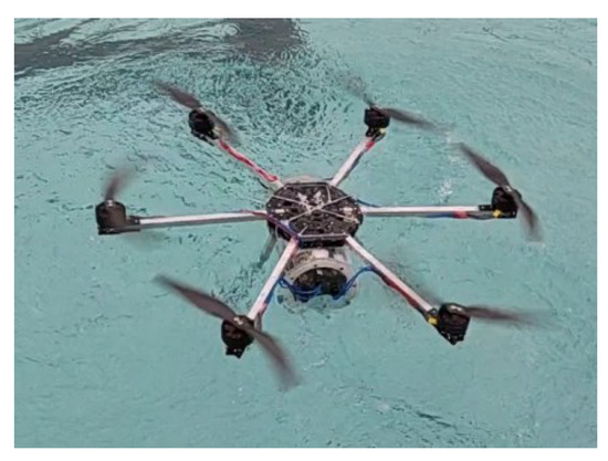
Figure 1.
Water and air amphibious multi-rotor UAV physical picture.
2. Dynamic and Kinematic Modeling
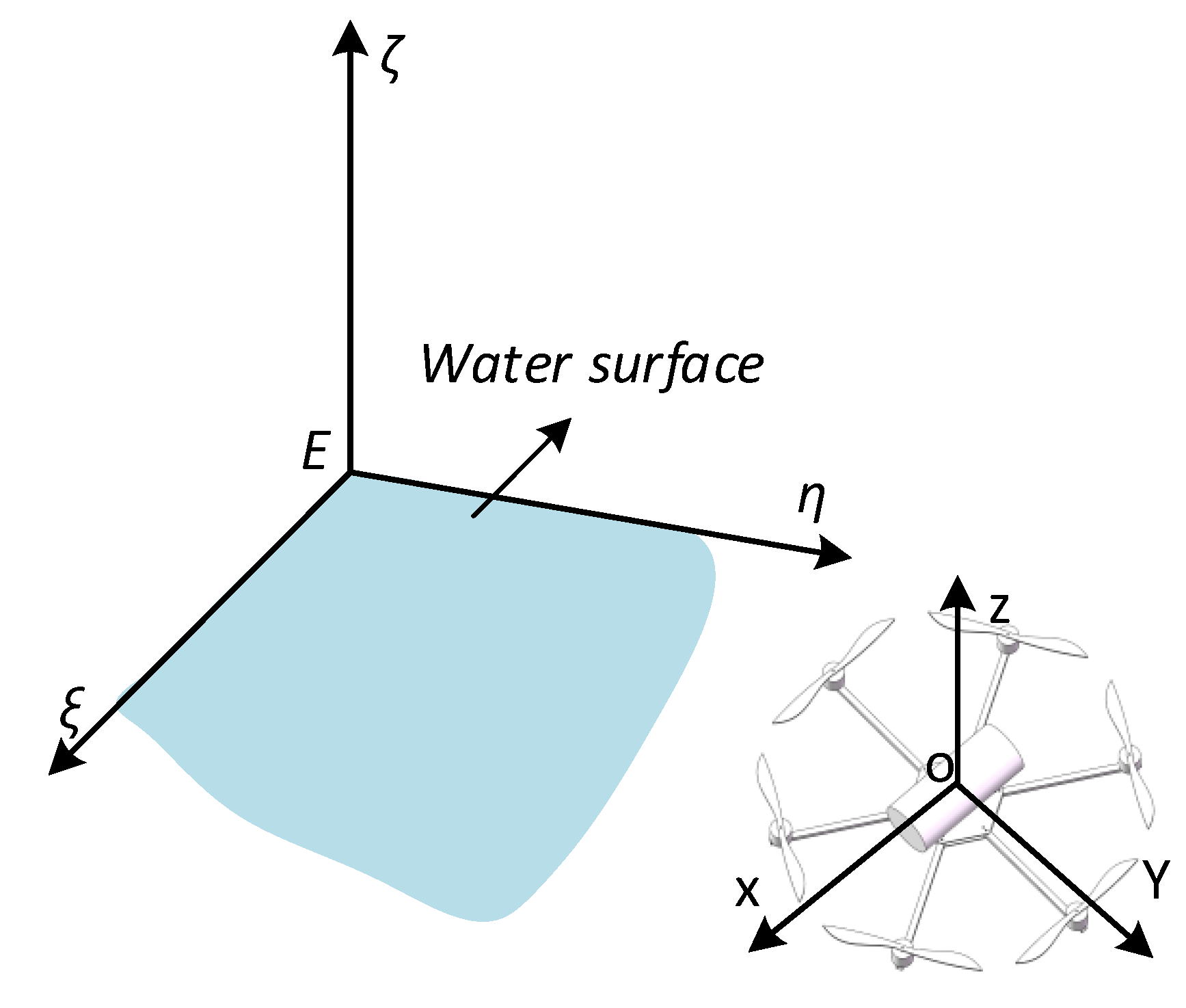
To facilitate the study of the dynamic and kinematic model of the amphibious multi-rotor UAV, this paper establishes a coordinate system as shown in Figure 2. is the coordinate system consisting of a fixed coordinate system established on the horizontal plane, and is an airframe motion coordinate system fixed on the amphibious multi-rotor UAV.

Figure 2.
Coordinate system.
First, to facilitate the analysis of the motion and forces on the amphibious multi-rotor UAV, the following assumptions are made for the amphibious multi-rotor UAV under study.
(1) The amphibious multi-rotor aircraft can be regarded as a rigid body with uniformly distributed mass and uniformly symmetric left and right.
(2) The center and center of gravity of the amphibious multi-rotor aircraft body coincide with the origin of the body coordinate system.
(3) There is a constant acceleration of gravity, ignoring the impact of the rotor on the surrounding airflow when the vehicle is in the air.
(4) The flow velocity of the water where the UAV is located is zero and the fluid is incompressible.
Second, before modeling, the symbols of physical quantities involved in this paper, including linear and angular velocities in the motion coordinate system, forces, and moments, and positions, linear velocities, and Euler angles in the fixed coordinate system, are defined as shown in Table 1.

Table 1.
Amphibious multi-rotor vehicle state physical quantities.
In a fixed coordinate system, according to the momentum theorem, the moment of momentum of the aircraft’s center of mass can be expressed as
where is the total force of the external forces on the amphibious multi-rotor UAV in a fixed coordinate system.
In addition, if the center of gravity of the amphibious multi-rotor UAV does not coincide with the origin of the coordinate system, according to the moment of momentum theorem, the moment of momentum of the rigid body to the point can be expressed as
where, is the momentum of the center of gravity , . According to the momentum moment theorem of rigid body, the total momentum moment of the amphibious multi-rotor UAV can be expressed as
Thus, according to the Newtonian Euler equation, it follows that
where, represents the total torque of UAV in the motion coordinate system.
In the motion coordinate system, since the center of gravity of the UAV coincides with the origin of the motion coordinate system,, , and . The general equations of motion of the UAV with six degrees of freedom in space in the moving coordinate system are obtained by calculating and simplifying according to Equations (1)–(4) and the momentum and momentum moment derivation theorems [34].
where , , and are the moments of inertia of the UAV in the three axes of the motion coordinate system.
3. Motion Force Analysis
The description of the relevant physical quantities in this chapter is shown in Table 2.
Table 2.
Description of related physical quantities.
Due to the need for a suitable and accurate force analysis of the amphibious multi-rotor UAV, and considering that the working environment of the amphibious multi-rotor UAV is variable and complex, this paper mainly considers the factors that play a major role in the system performance: static force (moment) , control force (moment) , and hydrodynamic force (moment) . Under normal conditions, the total external force (moment) on the amphibious multi-rotor UAV moving in the water is , where is the static force (moment) consisting of gravity and buoyancy; is the control force (moment) including rotor lift; is the hydrodynamic force (moment) caused by the motion of the amphibious multi-rotor UAV in the water. In this paper, it is stipulated that the force model is judged according to the position of the center of mass of the aircraft. When z > 0, the hydrodynamic force is ignored, and the static and dynamic models are judged according to the positive and negative values of z.
3.1. Static Force (Moment)
In the process of air motion, the static force on the vehicle is gravity, and the magnitude is ; in the process of underwater motion, the static forces include gravity and buoyancy , where gravity is expressed as ; buoyancy is expressed as , where is the fluid density in the basin, and is the amount of water discharged by the drone.
In the coordinate system , the combined force on the drone is , where , , and the center of gravity of the drone coincides with the origin of the object coordinates. When the center of gravity of the vehicle does not coincide with its floating center, the center of gravity and the center of buoyancy in the motion coordinate system are given as and , respectively.
Then the static force matrix (for the airframe coordinate system) on the UAV in a fixed coordinate system can be obtained as
3.2. Thrust (Moment)
The amphibious multi-rotor vehicle relies on its propulsion system for both underwater and aerial movements, as shown in Figure 3, for the location distribution of its propellers and the steering of its motors. The arrows in the figure point to the direction of rotation of the motor, and the direction of thrust generated is parallel to the axis.
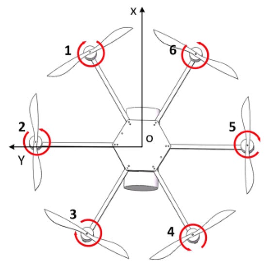
Figure 3.
Distribution of motors.
It is assumed that the propellers are fully submerged in a certain medium when the vehicle is operating, and the effects of factors such as fluid flow are ignored. Air propellers have also been shown to be effective in water [35]. The propeller thrust for any operating condition can be estimated using the empirical equation [36], then the thrust is
In the above equation, denotes the thrust coefficient of the propeller [37], where the subscripts and denote the type of propeller and the type of medium it is in, respectively. For example, denotes the propeller thrust coefficient used during the transition from air to water for an amphibious multi-rotor UAV; denotes the propeller speed, denotes the diameter of different types of propellers.
The propeller generates thrust through the rotating fluid, so the drive motor must generate enough torque to achieve rotational motion. This paper uses DC brushless motors, and their required drive torque can be calculated by the following empirical [17] formula:
In this equation, denotes the propeller moment coefficient [37]. Both thrust and moment coefficients are related to the geometric parameters of the propeller and the properties of the working medium and can be approximated empirically instead of in the actual modeling calculations.
Let the propeller speed of the propeller be , and the six propeller speeds be , then the thrust generated by the vehicle propeller system and its moment can be obtained as
In this equation, , , , and , where represent the thrust (moment) coefficients used in the air and underwater, respectively, and represent the distance from the motor to the origin of the motion coordinate system, .
3.3. Hydrodynamic (Moment)
Under normal conditions, the hydrodynamic forces (moments) are influenced by the physical characteristics, motion state, and fluid properties of the amphibious multi-rotor vehicle. Assumptions:
When the amphibious multi-rotor vehicle moves in water, it is subjected to hydrodynamic forces (moments) generated by the water flow on the surface of the vehicle. According to the principle of fluid dynamics, the hydrodynamic forces of the underwater robot consist of inertial hydrodynamic forces (moments) and viscous fluid hydrodynamic forces (moments) . Among them, the inertial hydrodynamic force is only related to acceleration and angular acceleration, and the viscous hydrodynamic force is only related to velocity and angular velocity.
3.3.1. Inertial Hydrodynamic Force (Moment)
According to the theory of fluid inertial forces, the hydrodynamic force on an object of any shape conducting non-constant motion in an ideal fluid, its magnitude is proportional to the (angular) acceleration of the object, the direction is opposite to the direction of acceleration, the proportionality constant is the added mass, the expression of inertial hydrodynamic force [38] is
After comprehensive consideration of the added mass, this paper approximates the amphibious multi-rotor UAV as a cylinder by ignoring its arm and motor. The vehicle is divided into strips based on the strip theory [39], and the two-dimensional hydrodynamic derivative of each strip is calculated. The integration operation is then performed on the two-dimensional hydrodynamic derivative to obtain the mass of the three-dimensional additional term. The added mass is also calculated using the empirical equation [40] to determine the added mass generated by the amphibious multi-rotor UAV during the underwater motion, which is expressed as
In this equation, is the added mass in the direction when moving with unit (angular) acceleration in the direction. represents the radius of the bottom circle of the cylindrical control chamber, and represents the length of the side of the cylinder at the control.
3.3.2. Viscous Hydrodynamic Force (Moment)
Due to fluid viscosity, the motion of a rigid body is also affected by viscous hydrodynamic forces , which are generated only with the velocity and angular velocity. The viscous hydrodynamic was obtained mainly by simulation. First, we consider the error between the actual hydrodynamics and the calculated hydrodynamics as an internal disturbance.
Then, the N-S equation together with the mode is solved using an implicit solver [41]. The flow field used in this paper is a rectangular parallel hexahedron of sufficient size. The final computational domain is obtained by a Boolean operation between the 3D model and the flow field. When the amphibious multi-rotor vehicle is moving slowly underwater, it is assumed to move along the Z-axis at . Through simulation, the relationship between the velocity and the combined force (moment) along the Z direction is shown in Table 3. Simulation tests show that when the amphibious multi-rotor vehicle comes out of the water, only viscous hydrodynamic forces exist in the Z direction, while the presence of forces and moments in other directions is negligible. Therefore, the relationship between the fitted velocity and the viscous hydrodynamic force is
Table 3.
Viscous hydrodynamic moment test table.
4. Controller Design
Amphibious multi-rotor UAVs are subject to hydrodynamic and other factors when moving underwater, which affects the stability of the controller. The disturbing factors become more complicated when the out-of-water movement is performed. To improve the anti-interference of the amphibious multi-rotor UAV, a cascade ADRC position and attitude controller is designed in this paper in combination with the ADRC algorithm [42], and the control block diagram is shown in Figure 4.
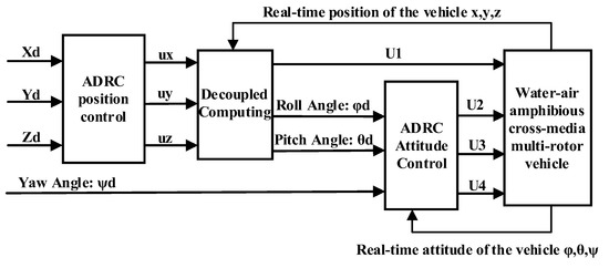
Figure 4.
ADRC control block diagram.
In the outgoing process, it is assumed that is the amount of variation due to buoyancy changes, is the error between the actual hydrodynamic forces experienced and the estimated hydrodynamic forces, and is the amount of other external disturbances experienced. Then, the external force (moment) applied in Equation (5) can be expressed as Equation (14):
The inner loop control includes pitch angle control, traverse angle control, and yaw angle control, assuming that is the given attitude angle and is the actual attitude angle obtained by feedback. The ADRC attitude controller design is introduced as an example of yaw angle control. Since the motion of the amphibious multi-rotor UAV is a small-angle motion in an equilibrium attitude, the angular velocity and attitude angle can be approximated by the quasi-integral relationship. The yaw angle control model is shown in Equation (15).
The ADRC arrangement transition process obtains the value of a given yaw angle from the outer ring.
In Equation (16), is the sampling time; is the factor that determines the tracking speed; is the filtering factor, and is the fast synthesis function of the second-order discrete system. After the expansion state observer and the nonlinear error feedback, the final control quantity is generated as in Equation (17).
In Equation (17), the dilated state observer of the ADRC obtains the observations of yaw angles and , , , and the system perturbations. is the parameter of the nonlinear function ; is the controller gain parameter; and is the output compensation factor. The complete ADRC formula can be found in reference [43].
The position of the controller design is according to the amphibious multi-rotor UAV ADRC attitude controller design method. In the coordinate system, the equation is satisfied as in Equation (18).
In Equation (18), is the external disturbance to the amphibious multi-rotor UAV in the coordinate system.
The external forces required to make the amphibious multi-rotor UAV reach the desired position are ; known and decoupled calculations are performed to obtain the magnitude of the external forces and attitude required to reach the desired position as in Equation (19).
In Equation (19), and are the calculated attitude sizes that the UAV needs to achieve to reach the desired position. Therefore, after obtaining and , the design process of yaw Angle controller is referred to. The controller of pitch Angle and roll Angle is designed as Formulas (20) and (21):
Since the mathematical model of the amphibious multi-rotor UAV is similar to that of ordinary quadcopters, the stability proof of the ADRC control system is similar to that in the literature [43,44].
5. Experimental Results and Analysis
To validate the accuracy of the motion model of the amphibious multi-rotor UAV and the effectiveness of the cascade ADRC position and attitude controller in the cross-media phase, a position and attitude controller was developed in this study using both the PID algorithm and SMC (sliding mode control) algorithm [45,46].
In the PID and SMC controller building, the design method of the ADRC controller is used, and the block diagram of the built cascade controller is similar to the block diagram of the ADRC controller in Figure 4.
The PID algorithm is a widely used control algorithm, and it is also widely used in aircraft control. It is based on error feedback, through the proportional, integral, and differential linear combination output control quantity to achieve the control effect. Using the altitude control of an amphibious aircraft as an example, its output control quantity is shown in Formula (22).
where is the running time of the experiment; , , are the proportion, integral and differential parameters to be determined, respectively; is the error between the expected height and the actual height at time t; is the output control quantity at time t.
The sliding mode control system is often used for aircraft control because of its strong robustness. In this paper, the sliding surface of the sliding mode controller is , using the constant velocity convergence law . In addition, to reduce the high-frequency jitter of the control signal, the function is used instead of , in the form shown in Equation (23). When the jitter condition of the output control signal is weak, it can be used as the final control quantity.
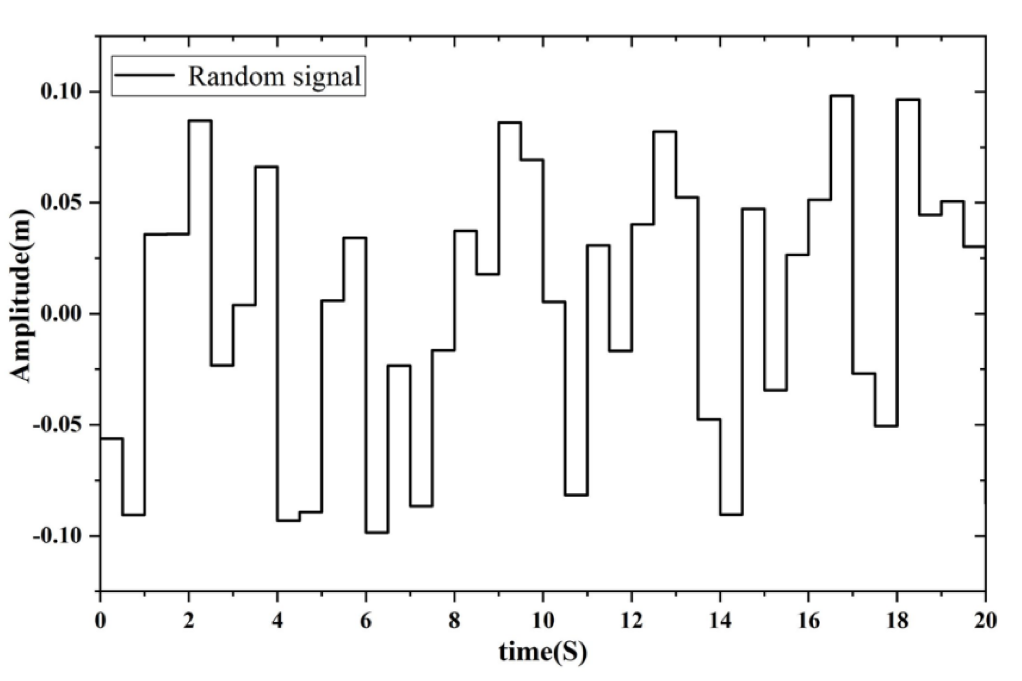
Equation (24) is used to simulate the disturbing external force during the motion across the medium. Additionally, considering the position offset generated by the amphibious multi-rotor UAV due to wave surge during underwater waves, this paper uses the random signal as shown in Figure 5 to represent the position offset and add it to the simulation position control loop.
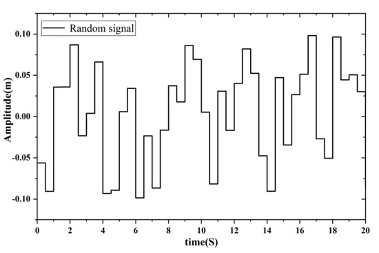
Figure 5.
Random offset.
The physical parameters of the amphibious multi-rotor UAV and the parameters designed for the simulation experiments are shown in Table 4.
Table 4.
Simulation parameters.
A simulation experiment using MATLAB with a simulation time of 15 s; given the initial position and the desired position ; initial positions of , , and , and desired positions of , and . The parameters of the PID controller and SMC controller are also adjusted to show better control performance, and the parameters of the ADRC controller are adjusted to meet the control requirements. The final simulation results are shown in Figure 6 and Figure 7.
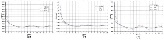
Figure 6.
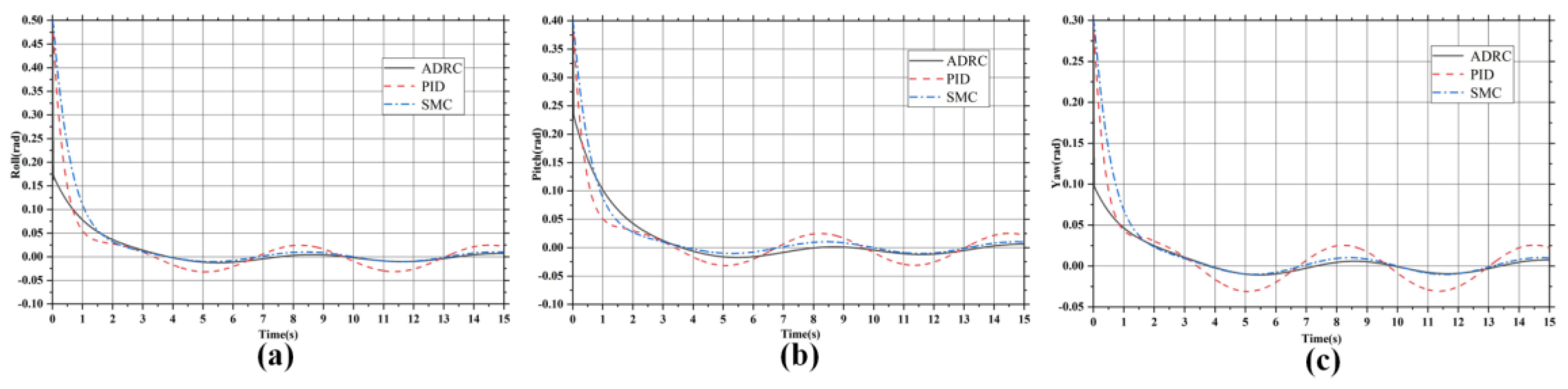
Simulation results of PID, SMC and ADRC out-of-water motion attitude angle control: (a) roll angle, (b) pitch angle, (c) yaw angle.
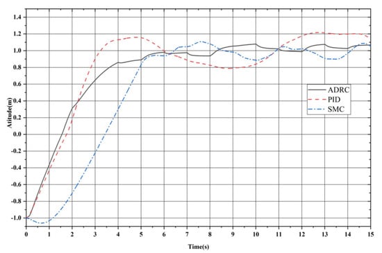
Figure 7.
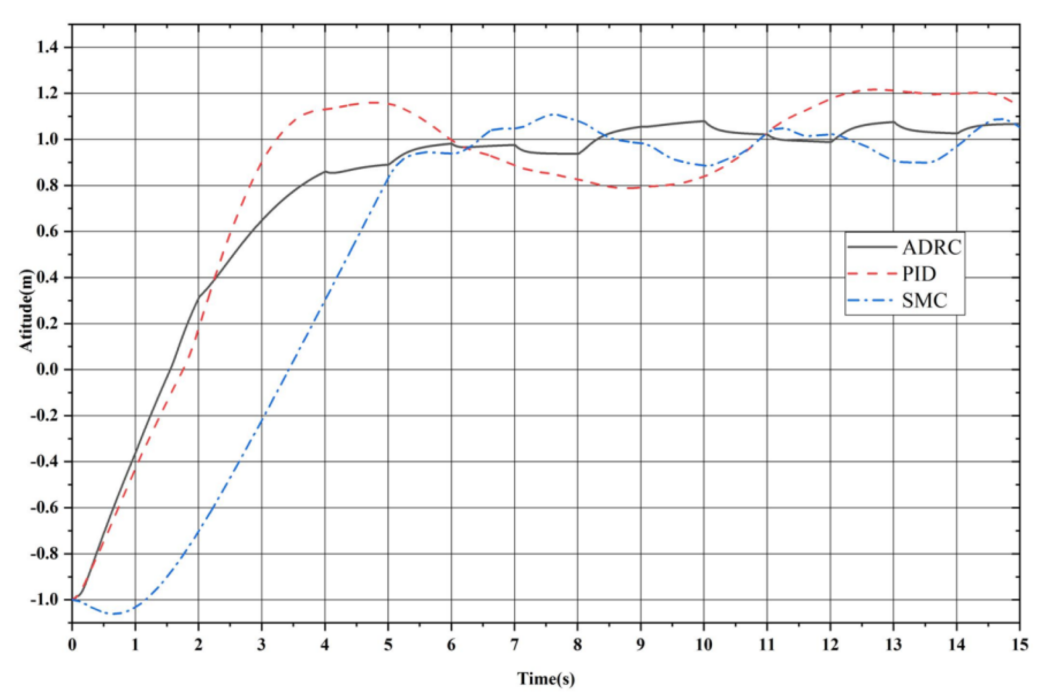
Comparison of simulation results of PID, SMC, and ADRC outgoing water motion height control.
From the simulation results of the attitude angle control in Figure 6, it can be found that PID, SMC, and ADRC can all bring the attitude of the UAV to the set desired attitude in about 3–4 s and keep the attitude in the vicinity of the desired attitude. It can also be found that after 4 s, the PID control curve has an obvious fluctuation compared with SMC and ADRC, and the fluctuation range is ; the SMC and ADRC control curve is relatively flat, and the fluctuation range is ; for the attitude control of the water exit process, PID and SMC and ADRC can all complete the effective control of the UAV attitude, but the anti-interference ability of the PID algorithm is weaker than SMC and ADRC.
From the simulation results of the altitude control in Figure 7, we can find that PID, SMC, and ADRC can all complete the altitude control of UAV. The time for the PID to reach the desired height for the first time is 3 s, which has better rapidity compared with SMC and ADRC, but the control curve of the PID is more fluctuating, with a fluctuation range of and an obvious amount of overshoot. The time for SMC and ADRC to reach the desired height for the first time is 6 s. Although there is a small reduction in rapidity, the fluctuation of the SMC control curve is smaller, and the fluctuation range is , and there is a reduction in overshoot, which also reflects better anti-interference performance. The fluctuation range of the ADRC control curve is , the minimum amount of fluctuation in the three controllers, and there is no overshoot when the UAV just reaches the desired altitude. In the form of disturbing external force as a sinusoidal signal, the fluctuation trend of the ADRC curve is not obvious compared with PID and SMC, which also shows the strong anti-disturbance property of the ADRC algorithm.
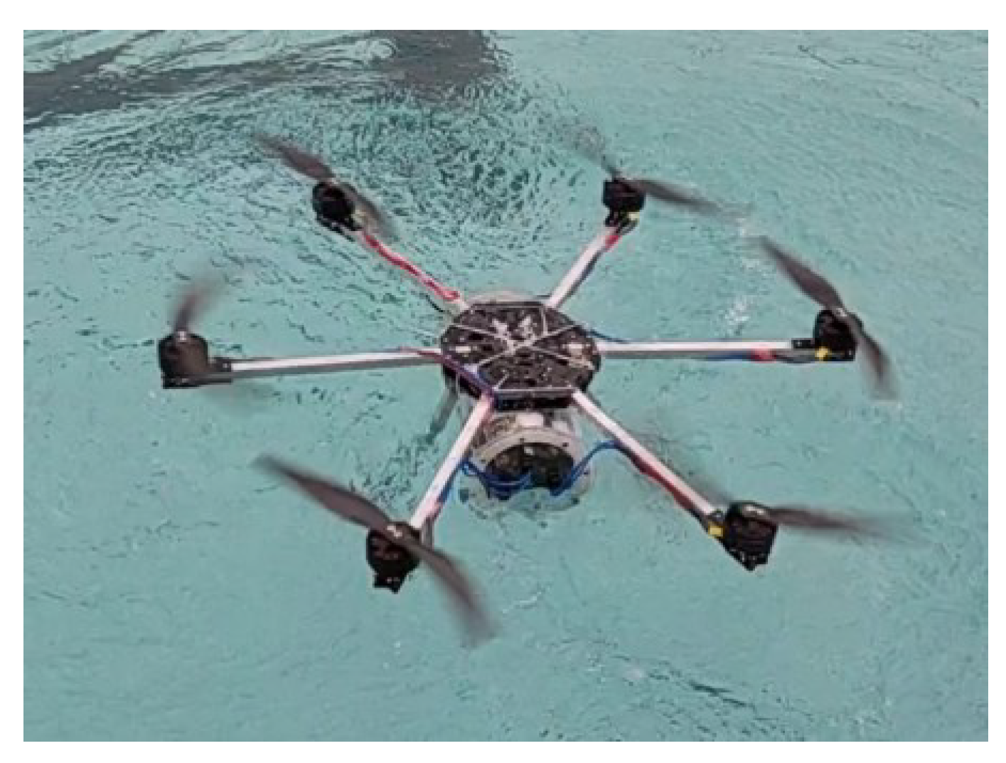
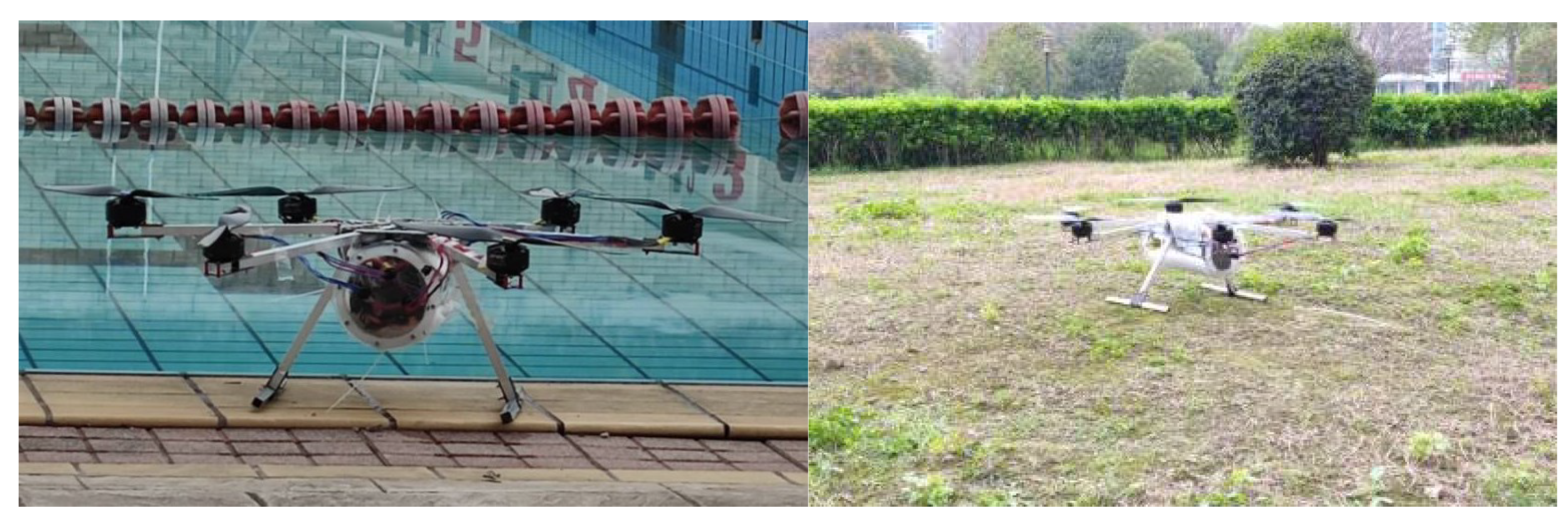
Furthermore, to verify the usability of the ADRC algorithm in an actual control, a control research process of ADRC is further carried out for the prototype of the amphibious multi-rotor UAV, as shown in Figure 8. In Figure 8, all electrical components are placed in a cylindrical waterproof compartment of acrylic material, and perforated screws are used to connect the wires to the inner and outer elements, and finally the gaps in the perforated screws are filled with waterproof glue to prevent water leakage. In addition, the brushless motors used in the prototype can work normally in water. The total memory of the ADRC controller is about 1881 KB, and it has high scalability.
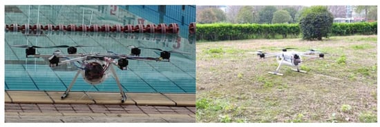
Figure 8.
Experimental prototype of an amphibious multi-rotor UAV.
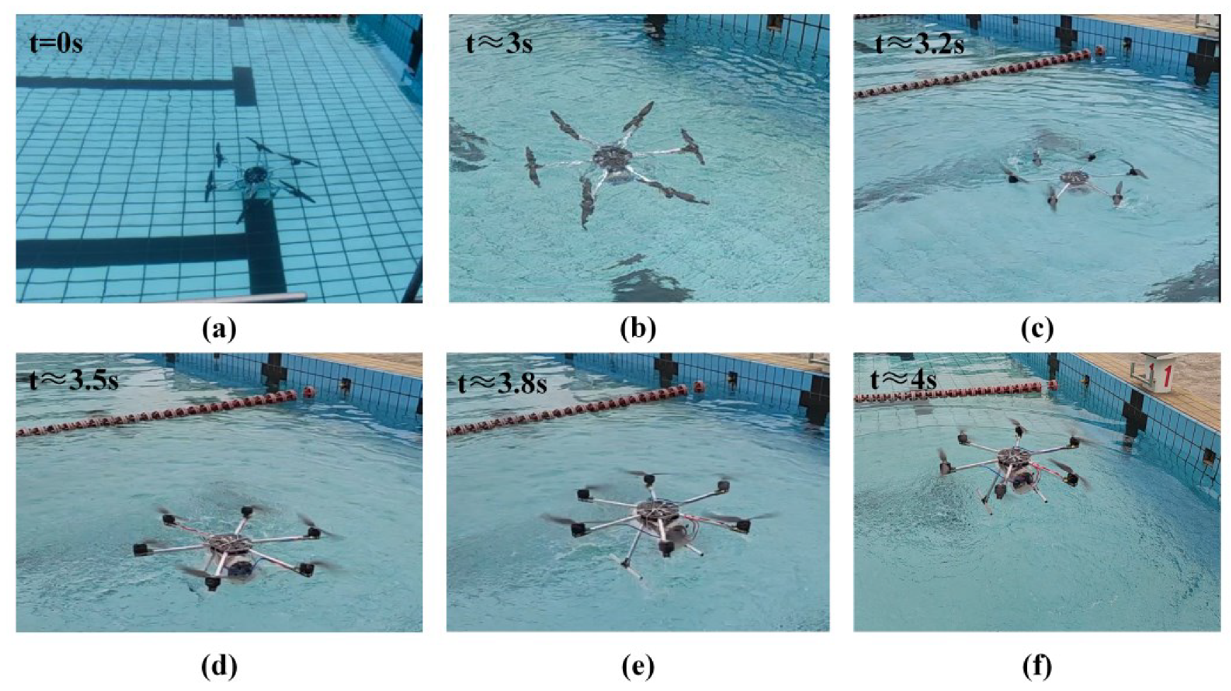
To verify the usability of the ADRC algorithm in a practical control, the amphibious multi-rotor UAV is placed at a depth of 1 m underwater, and the initial attitude , , is set. In the state of the body so set, the controller built with PID, SMC, and ADRC algorithms are used to control the water discharge to a height of 1 m in the air, respectively. The whole process of amphibious multi-rotor UAV out-of-water movement is shown in Figure 9. The experimental results are shown in Figure 10 and Figure 11.

Figure 9.
Diagram of the out-of-water motion process: (a) 1 m underwater (b) from underwater near the horizontal (c), (d) transition (e) 0–1 m in air (f) 1 m in air.
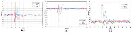
Figure 10.
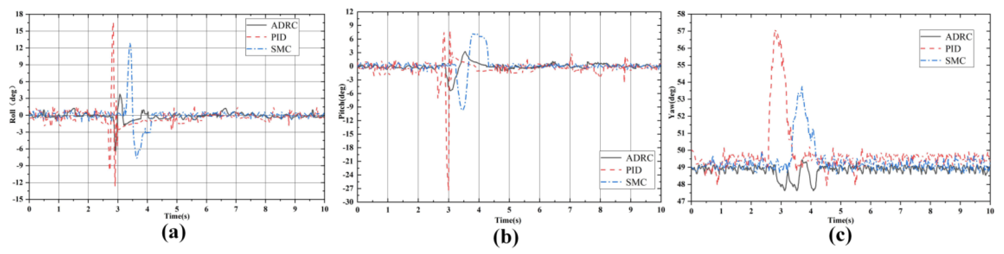
Experimental results of attitude angle control of PID, SMC, and ADRC out-of-water motion: (a) roll angle, (b) pitch angle, (c) yaw angle.
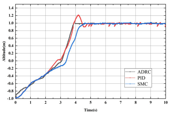
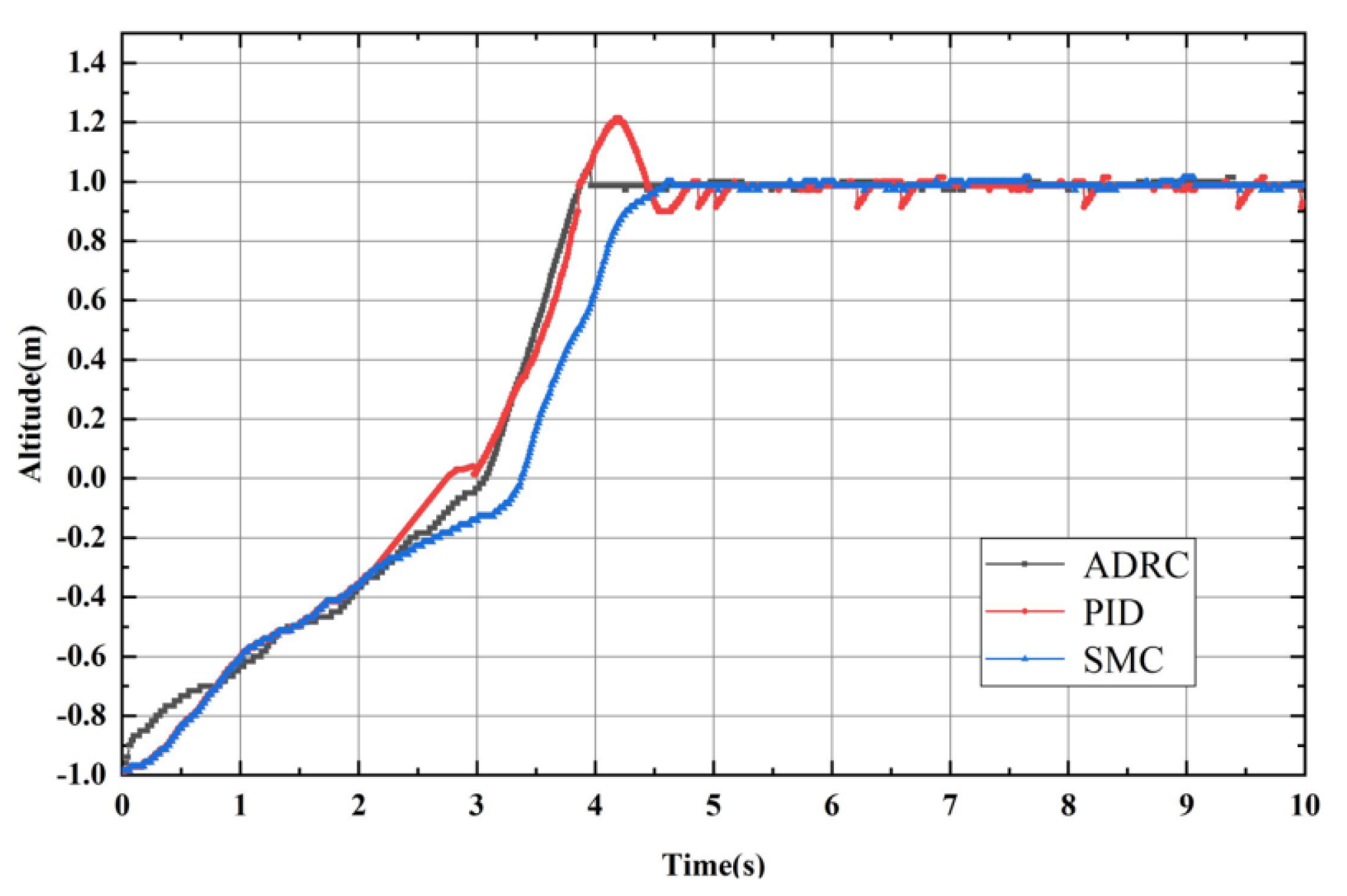
Figure 11.
Comparison of experimental results of PID, SMC, and ADRC water outlet motion height control.
From the experimental results in Figure 10, it can be found that near 3 s, i.e., when the amphibious multi-rotor UAV is out of the water transition, the attitude of the UAV has a more serious jitter due to the buoyancy and hydrodynamic force and the weight of the water attached to the airframe. ADRC allows the UAV roll angle and pitch angle jitter to be controlled between and . SMC can make the UAV roll angle and pitch angle jitter be controlled between and . The PID allows the UAV roll angle and pitch angle jitter to be controlled between and . It can be found that ADRC still shows strong control performance in the actual control and can achieve good attitude control to ensure the stable completion of the water exit movement. SMC performance can also meet the actual control needs, but the anti-interference is weaker compared to ADRC. PID has the worst performance, and in the actual process, the PID attitude control may cause the fuselage to tilt excessively, making the propeller hit the horizontal surface, causing the UAV to flip sideways and fall into the water, leading to the failure of the out-of-water movement.
From the comparison of the experimental results of out-of-water motion in Figure 11, PID, SMC, and ADRC have completed the out-of-water motion of the amphibious multi-rotor UAV. However, the PID algorithm has a significant overshoot of 0.2 m; the SMC is slower and reaches the desired height at 4.5 s, but there is no significant overshoot, and the control curve is smoother; the ADRC reaches the desired height at 4 s and there is no overshoot, and the control curve is very smooth.
Based on the out-of-water motion control of an amphibious aircraft, it can be seen that before reaching z = 0, since the model parameters did not change significantly and the controller parameters were adjusted to the optimal condition for the experiment, the control curve of the three control algorithms, PID, SMC, and ADRC, all showed a certain anti-interference ability against external disturbances. When the aircraft reaches z > 0, the force situation changes dramatically, and the PID controller curve jumps up and down at 3 s, indicating the aircraft wobbles at the water–air interface, which may lead to the amphibious aircraft’s rotor flaps to the horizontal plane resulting in the amphibious aircraft rolling over and falling into the water. Finally, the PID algorithm also generates a large overshoot of 0.2 m, which indicates that the PID algorithm cannot overcome the instability caused by the change in model parameters. The control curve of the SMC algorithm is smooth and shows no obvious overkill. However, there is a 0.5 s delay in the control effect when dynamic models and parameter switching occur. Compared with the control curve of the ADRC algorithm and PID algorithm, it can be considered that part of the control rapidity is sacrificed and the control robustness is improved. Compared with the PID algorithm and SMC algorithm, the control curve of the ADRC algorithm exhibits no significant step changes after the amphibious aircraft transitions from water to air. Furthermore, the control curve remains smooth without any noticeable overshoot. On the premise that the robustness of the control algorithm is guaranteed, good control rapidity is also retained.
ADRC is proposed based on the shortcomings and improvement methods of PID, and the emergence of ADRC solves some limitations of PID to a certain extent, making the control system more stable, adaptable, and accurate. Therefore, in the simulation and experiments, ADRC and PID have the same speed, and ADRC has a lower overshoot and stronger anti-interference ability than PID. In terms of the control performance for ADRC and SMC, ADRC introduces a state observer to observe and estimate the total disturbance in real time and compensate at the input to eliminate interference more effectively, and ADRC has a stronger adaptive ability to dynamically adjust parameters to adapt to a different system and environmental changes. For SMC, it focuses more on suppressing interference. Therefore, in the simulation and experiments, ADRC has a slightly better anti-interference ability than SMC and has a shorter rise time than SMC. Therefore, through both the simulation and experiments, this paper verifies the excellence of the proposed method.
6. Conclusions
For the amphibious multi-rotor UAV, the water–air transition presents a significant challenge due to changes in buoyancy and added mass as well as the impact of the “water surface effect”. To address this challenge, this paper proposes the use of the conventional ADRC control algorithm, which has shown strong robustness in aircraft control, to design the controller for the amphibious multi-rotor UAV and conduct a preliminary exploration of cross-media control research. Kinematic and dynamic models of the amphibious multi-rotor UAV were established, and the hydrodynamics of the underwater vehicle were analyzed to construct a cascaded active anti-interference controller using the ADRC algorithm. Simulation results demonstrate that the ADRC algorithm provides better control performance and robustness than SMC and PID in the cross-media control process. Experimental verification is then carried out to verify the usability of the ADRC algorithm in actual control. The results show that during the water discharge process, although the amphibious multi-rotor UAV experiences significant disturbance, the ADRC algorithm demonstrates smaller attitude fluctuations compared to SMC and PID, as well as better control performance and robustness. These results verify the superiority of the ADRC control algorithm and demonstrate its potential for use in the design of a cross-media controller for the amphibious multi-rotor UAV.
Author Contributions
Conceptualization, L.T.; Methodology, S.L.; Validation, L.L.; Resources, J.H.; Writing—original draft, L.T.; Writing—review & editing, Z.Q. and H.S. All authors have read and agreed to the published version of the manuscript.
Funding
This work was supported by the Science Fund for Excellent Young Scholars of Heilongjiang Province under Grant YQ2020F007, the National Natural Science Foundation of China under Grant 6191101340, the China Postdoctoral Science Foundation funded under Grant 2018M631930, and Fundamental Research Funds for the Central Universities under Grant 2022FRFK060007.
Data Availability Statement
The data that support the findings of this study are available from the corresponding author upon reasonable request.
Conflicts of Interest
The authors declare no conflict of interest.
References
- Yang, X.G.; Liang, J.H. Status of research on water-air amphibious trans-media unmanned aerial vehicles. Robotics 2018, 40, 102–114. [Google Scholar]
- Zeng, Z.; Lyu, C.; Bi, Y. Review of hybrid aerial underwater vehicle: Cross-domain mobility and transitions control. Ocean Eng. 2022, 248, 110840. [Google Scholar] [CrossRef]
- Zhang, Y.; Chen, X.; Zhou, J. Flight design and dynamics analysis of a new water-air UAV. J. Phys. Conf. Ser. 2021, 1748, 062023. [Google Scholar] [CrossRef]
- Lu, D.; Xiong, C.; Zhou, H. Design, fabrication, and characterization of a multimodal hybrid aerial underwater vehicle. Ocean Eng. 2021, 219, 108324. [Google Scholar] [CrossRef]
- Maia, M.M.; Soni, P.; Diez, F.J. Demonstration of an aerial and submersible vehicle capable of flight and underwater navigation with seamless air-water transition. arXiv 2015, arXiv:1507.01932. [Google Scholar]
- Ma, Z.; Chen, D.; Li, G.; Zhou, J. Constrained adaptive backstepping take-off control for a morphing hybrid aerial underwater vehicle. Ocean. Eng. 2020, 213, 107666. [Google Scholar]
- Chen, G.; Liu, A.; Hu, J.; Feng, J.; Ma, Z. Attitude and altitude control of unmanned aerial-underwater vehicle based on incremental nonlinear dynamic inversion. IEEE Access 2020, 8, 156129–156138. [Google Scholar] [CrossRef]
- Lu, D.; Xiong, C.; Zeng, Z. Adaptive dynamic surface control for a hybrid aerial underwater vehicle with parametric dynamics and uncertainties. IEEE J. Ocean. Eng. 2019, 45, 740–758. [Google Scholar] [CrossRef]
- Drews, P.L.J.; Neto, A.A.; Campos, M.F.M. Hybrid unmanned aerial underwater vehicle: Modeling and simulation. In Proceedings of the 2014 IEEE/RSJ International Conference on Intelligent Robots and Systems, Chicago, IL, USA, 14–18 September 2014; pp. 4637–4642. [Google Scholar]
- Neto, A.A.; Mozelli, L.A.; Drews, P.L.J.; Campos, M.F.M. Attitude control for an hybrid unmanned aerial underwater vehicle: A robust switched strategy with global stability. In Proceedings of the 2015 IEEE International Conference on Robotics and Automation (ICRA), Seattle, WA, USA, 26–30 May 2015; pp. 395–400. [Google Scholar]
- Yu, Z.J.; Feng, J.F.; Hu, J.H.; Wei, Y.M. Modeling of water-air spanning navigators out of water motion. Comput. Simul. 2015, 32, 101–105. [Google Scholar]
- Siddall, R.; Ortega Ancel, A.; Kovač, M. Wind and water tunnel testing of a morphing aquatic micro air vehicle. Interface Focus 2017, 7, 20160085. [Google Scholar] [CrossRef]
- Qi, D.; Feng, J.; Li, Y. Dynamic model and ADRC of a novel water-air unmanned vehicle for water entry with in-ground effect. J. Vibroeng. 2016, 18, 3743–3756. [Google Scholar] [CrossRef]
- Ma, Z.; Feng, J.; Yang, J. Research on vertical air-water trans-media control of hybrid unmanned aerial underwater vehicles based on adaptive sliding mode dynamical surface control. Int. J. Adv. Robot. Syst. 2018, 15, 1729881418770531. [Google Scholar] [CrossRef]
- Mercado Diego Maia, M.M.; Diez, F.J. Modeling and control of unmanned aerial/underwater vehicles using hybrid control. Control. Pract. 2018, 76, 112–122. [Google Scholar] [CrossRef]
- Zha, J.; Thacher, E.; Kroeger, J.; Makiharju, S.A.; Mueller, M.W. Towards breaching a still water surface with a miniature unmanned aerial underwater vehicle. In Proceedings of the 2019 International Conference on Unmanned Aircraft Systems (ICUAS), Atlanta, GA, USA, 11–14 June 2019; IEEE: New York, NY, USA, 2019; pp. 1178–1185. [Google Scholar]
- Yan, Q.M.; Hu, J.H. Modeling and control of water-air crossing for a double-layer quadrotor trans-media vehicle. Flight Mech. 2020, 38, 7. [Google Scholar]
- Zhang, S.; Zhang, S.X. Fast water-air transition design and test for small cross-media UAV. Flight Mech. 2021, 39, 77–81. [Google Scholar]
- Chen, Q.; Zhu, D.; Liu, Z. Attitude control of aerial and underwater vehicles using single-input FUZZY P+ ID controller. Appl. Ocean Res. 2021, 107, 102460. [Google Scholar] [CrossRef]
- Ma, Z.C.; Jing, X.Y.; Zhang, Z.R.; Xiao, S.; Zhao, T.; Li, G. GA and RBFNN based PID for altitude-depth control of the multirotor hybrid aerial underwater vehicles. J. Phys. Conf. Ser. 2022, 2239, 012005. [Google Scholar]
- Ma, Z.; Chen, D.; Li, G.; Jing, X.; Xiao, S. Configuration design and trans-media control status of the hybrid aerial underwater vehicles. Appl. Sci. 2022, 12, 765. [Google Scholar] [CrossRef]
- Rafeeq, M.; Toha, S.F.; Ahmad, S.; Razib, M.A. Locomotion strategies for amphibious robots-a review. IEEE Access 2021, 9, 26323–26342. [Google Scholar] [CrossRef]
- Raja, V.; Kumar, A.; Pacheco, D.A.J. Multi-disciplinary engineering design of a high-speed nature-inspired unmanned aquatic vehicle. Ocean. Eng. 2023, 270, 113455. [Google Scholar] [CrossRef]
- Abro, G.E.M.; Bin Mohd Zulkifli, S.A.; Asirvadam, V.S. dual-loop single dimension fuzzy-based sliding mode control design for robust tracking of an underactuated quadrotor craft. Asian J. Control. 2023, 25, 144–169. [Google Scholar] [CrossRef]
- Suhail, S.A.; Bazaz, M.A.; Hussain, S. Adaptive sliding mode-based active disturbance rejection control for a quadcopter. Trans. Inst. Meas. Control. 2022, 44, 3176–3190. [Google Scholar] [CrossRef]
- Meng, Z.; Yang, X.; Ding, S. The controller design of the water-aerial vehicle based on variable gain PID. In Proceedings of the 2020 Chinese Control And Decision Conference (CCDC), Hefei, China, 22–24 August 2020; pp. 4590–4594. [Google Scholar]
- El-kenawy, E.S.M.; Ibrahim, A.; Bailek, N. Sunshine duration measurements and predictions in Saharan Algeria region: An improved ensemble learning approach. Theor. Appl. Climatol. 2021, 147, 1015–1031. [Google Scholar] [CrossRef]
- Ibrahim, A.; Mirjalili, S.; El-Said, M.; Ghoneim, S.; Al-Harthi, M. Wind speed ensemble forecasting based on deep learning using adaptive dynamic optimization algorithm. IEEE Access 2021, 9, 125787–125804. [Google Scholar] [CrossRef]
- Huo, Y.; Li, Y.; Feng, X. Memory-based reinforcement learning for trans-domain tiltrotor robot control. J. Phys. Conf. Ser. 2020, 1510, 012011. [Google Scholar] [CrossRef]
- Shen, S.; Xu, J. Attitude active disturbance rejection control of the quadrotor and its parameter tuning. Int. J. Aerosp. Eng. 2020, 2020, 8876177. [Google Scholar] [CrossRef]
- Song, Z.; Wang, Y.; Liu, L. Research on attitude control of quadrotor uav based on active disturbance rejection control. In Proceedings of the 2020 Chinese Control And Decision Conference (CCDC), Hefei, China, 22–24 August 2020; pp. 5051–5056. [Google Scholar]
- Wang, Y.; Li, J.; Huo, J. Analysis of the hydrodynamic performance of a water-air amphibious trans-medium hexacopter. In Proceedings of the 2020 Chinese Automation Congress (CAC), Shanghai, China, 6–8 November 2020; pp. 4959–4964. [Google Scholar]
- Li, J.; Chen, S.; Guo, M. Underwater dynamics modeling and simulation analysis of trans-media multicopter. In Proceedings of the 2021 5th International Conference on Robotics and Automation Sciences (ICRAS), Wuhan, China, 11–13 June 2021; pp. 116–122. [Google Scholar]
- Lu, D.; Xiong, C.; Lyu, B. Multi-mode hybrid aerial underwater vehicle with extended endurance. In Proceedings of the 2018 OCEANS-MTS/IEEE Kobe Techno-Oceans (OTO), Kobe, Japan, 28–31 May 2018; pp. 1–7. [Google Scholar]
- Alzu’bi, H.; Akinsanya, O.; Kaja, N. Evaluation of an aerial quadcopter power-plant for underwater operation. In Proceedings of the 2015 10th International Symposium on Mechatronics and its Applications (ISMA), Sharjah, United Arab Emirates, 8–10 December 2015; pp. 1–4. [Google Scholar]
- Chen, Y.; Liu, Y.; Meng, Y. System modeling and simulation of an unmanned aerial underwater vehicle. J. Mar. Sci. Eng. 2019, 7, 444. [Google Scholar] [CrossRef]
- Shi, D.; Dai, X.; Zhang, X. A practical performance evaluation method for electric multicopters. IEEE/ASME Trans. Mechatron. 2017, 22, 1337–1348. [Google Scholar] [CrossRef]
- Meng, L.; Yang, L.; Su, T.C. Study on the influence of porous material on underwater vehicle’s hydrodynamic characteristics. Ocean. Eng. 2019, 191, 106528. [Google Scholar] [CrossRef]
- Isa, K.; Arshad, M.R.; Ishak, S. A hybrid-driven underwater glider model, hydrodynamics estimation, and an analysis of the motion control. Ocean. Eng. 2014, 81, 111–129. [Google Scholar] [CrossRef]
- Ross, A.; Fossen, T.I.; Johansen, T.A. Identification of underwater vehicle hydrodynamic coefficients using free decay tests. IFAC Proc. Vol. 2004, 37, 363–368. [Google Scholar] [CrossRef]
- He, J.W.; Zhai, J.Y.; Gao, W.P.; Li, Y. Numerical simulation of flow characteristics of cylindrical structure of underwater navigable body based on different turbulence models. J. Mil. Eng. 2022, 43, 53–63. [Google Scholar]
- Shi, J.; Pei, Z.G.; Tang, Z.Y. Design and implementation of improved active disturbance rejection quadrotor UAV control system. J. Beijing Univ. Aeronaut. Astronsutics 2021, 47, 1823–1831. [Google Scholar]
- Zhang, Y.; Chen, Z.; Zhang, X. A novel control scheme for quadrotor UAV based upon active disturbance rejection control. Aerosp. Sci. Technol. 2018, 79, 601–609. [Google Scholar] [CrossRef]
- Song, Z.; Zhao, C.; Zhang, H.; Dong, T.; Ma, A.; Yan, D. Research on aircraft attitude control method based on linear active disturbance rejection. Int. J. Aerosp. Eng. 2022, 2022, 1908020. [Google Scholar] [CrossRef]
- Zhou, L.; Pljonkin, A.; Singh, P.K. Modeling and PID control of quadrotor UAV based on machine learning. J. Intell. Syst. 2022, 31, 1112–1122. [Google Scholar] [CrossRef]
- Zheng, B.; Wu, Y.; Li, H. Adaptive sliding mode attitude control of quadrotor uavs based on the delta operator framework. Symmetry 2022, 14, 498. [Google Scholar] [CrossRef]


Disclaimer/Publisher’s Note: The statements, opinions and data contained in all publications are solely those of the individual author(s) and contributor(s) and not of MDPI and/or the editor(s). MDPI and/or the editor(s) disclaim responsibility for any injury to people or property resulting from any ideas, methods, instructions or products referred to in the content. |
© 2023 by the authors. Licensee MDPI, Basel, Switzerland. This article is an open access article distributed under the terms and conditions of the Creative Commons Attribution (CC BY) license (https://creativecommons.org/licenses/by/4.0/).