Abstract
The article assesses comparative analyses of some selected machine-learning algorithms for the estimation of the subsurface tensile strength of cementitious composites containing waste granite powder. Any addition of material to cementitious composites causes their properties to differ; therefore, there is always a need to prepare a precise model for estimating these properties’ values. In this research, such a model of prediction of the subsurface tensile strength has been carried out by using a hybrid approach of using a nondestructive method and neural networks. Moreover, various topologies of neural networks have been evaluated with different learning algorithms and number of hidden layers. It has been proven by the very satisfactory results of the performance parameters that such an approach might be used in practice. The errors values (MAPE, NRMSE, and MAE) of this model range from 10 to 12%, which, in the case of civil engineering practice, proves that this model is sufficient for being used. This novel approach can be a reasonable alternative for evaluating the properties of spacious cementitious composite elements where there is a need to analyse not only the compressive strength but also its subsurface tensile strength.
1. Introduction
A composite is defined as a material made up of at least two components with different properties such that it has superior and/or new properties over those components taken separately. However, the given definition is not generally accepted and precise, but is intended to generalize the most common descriptive definitions. On its basis, it can be assumed that a cement composite is a composite of whom one of the basic components is cement. The most popular composites in which cement acts as a binder are: grout, mortar, and concrete [1]. By the term grout, we mean the material that results from the combination of water and cement. The leaven itself is rarely used in construction. Cement mortar is used much more often, e.g., for bricklaying, plastering, or making floor underlays. Standard cement mortar is a mixture of the appropriate proportions of cement, water, and sand. The composition of the mortar can be supplemented with additives and admixtures added to give the appropriate properties to the mixture or hardened mortar. Concrete is another material. It is the most widespread cement composite in the world. In addition to water, sand, and cement, concrete contains coarse aggregate. In concrete, as in the case of mortar, we use admixtures and additives, which, in standard concretes, allow us, for example, to obtain better working parameters of the mixture with the use of less water, or to improve the physical parameters of the hardened composite [2].
An additive to concrete can be called a fine-grained component added to the concrete mix, whose task is to improve its properties or obtain the special parameters of hardened concrete. The amount of additive is generally from 5% to 15% of the weight of the cement. The content of the additive should be taken into account in subsequent iterations of the calculations of the designed mixtures. There are two main types of additives. The first type is nearly inert additives, which are in turn divided into fillers and pigments. Pigments are used to tint the concrete to the desired color. The role of fillers is to fill the pores of the concrete mixture [3]. An additive typical for this group is limestone powder. Additives with latent hydraulic or pozzolanic properties are the second type of concrete additives. Their use leads to an improvement in the properties of concrete or the acquisition of special properties. Representatives of this group are silica fume or fly ash. The most popular methods of adding fillers to a cement composite are in the form of (i) cement replacement, (ii) aggregate replacement, and (iii) grout replacement. These methods are successfully applied to waste materials in the form of quartz dust, marble powder, powdered glass, or fly ash, added to concrete and mortar as fillers or additives that modify the properties of the mixture or the hardened cement composite [4].
The mere production of cement as a basic component of concretes and mortars also has an undesirable impact on the environment. During the production of 1 ton of this material, about 900 kg of carbon dioxide are emitted; therefore, the partial replacement of cement with another component may contribute to reducing CO2 emissions to the atmosphere [5].
Granite powder is a waste material that results from the crushing or cutting of granite rocks for industrial purposes. In recent years, an increase in the amount of granite powder waste has been observed as a result of the development of the granite industry. The powder fraction of this material alone is currently not applicable, which exacerbates the problem of the proper management of this product. The improper storage of dry material in the form of heaps, which can easily spread in the environment, causes water pollution, changes in the pH of land intended for agricultural purposes, and air pollution in the vicinity of landfills. Insisting that the effects of the environmental degradation by granite powder can be felt directly by humans, it is necessary to take the appropriate measures to reduce the amount of this production residue in the environment. One way to reduce its harmful effects is to use this by-product for the sustainable production of cement composites as the most common building material and use it as a supplementary cementitious material (SCM) [6].
However, when another material is added to cementitious composites, it is necessary to evaluate how it affects their properties. Most of the tests used for evaluating the materials’ properties in civil engineering are destructive; therefore, they are costly and time-consuming, and they produce wastes. Therefore, sometimes for this purpose, the nondestructive tests are reasonable substitutes [7]. It is also important while performing such tests in buildings which are operating or which are characterized as historical heritage sites and cannot be tested destructively [8]. It was previously shown that an NDT method such as the Schmidt hammer method was successful in evaluating the compressive strength of concrete [9,10]. However, there is an issue with evaluating the other properties of cementitious composites such as subsurface tensile strength. For this purpose, very often, a method such as the pull-off test is used, but, after the test, the sample needs to be repaired, which makes this method not fully nondestructive [11]. However, it is still possible to try to correlate the compressive strength with the subsurface tensile strength. Therefore, it is possible to try to evaluate the opposite, which means that it is possible to evaluate the subsurface tensile strength using a Schmidt hammer [12]. Evaluating the subsurface tensile strength in cementitious composites such as mortars dedicated for floor substrate is very important because of the fact that, very often, these parameters are responsible for the durability of the element [13].
Recently, very often, soft computing techniques such as artificial neural networks are used for this purpose, while they are able to strengthen the results of NDT methods by improving the performance of these methods, which might be necessary in this case [14]. Such approaches have previously been successful when using the combination of a Schmidt hammer and neural networks to predict the unconfined compressive strength of rocks [15], to predict the damage analyses of concrete subjected to high temperature [16], or to assess the load-carrying capacity of concrete anchor bolts [17].
Taking the aforementioned thoughts into account, it might be reasonable to use such a combination for evaluating the subsurface tensile strength of cementitious composites using the combination of a Schmidt hammer and neural networks. Therefore, for this purpose, the authors propose the hybrid method of using the nondestructive Schmidt hammer method and neural networks for evaluating the properties of cementitious composites containing granite powder that can be used in the civil-engineering practice. This solution might be beneficial for evaluating the properties of existing floors made of mortars which are located in operating buildings.
2. Materials and Methods
2.1. Materials
In order to create the database used for ANN modeling, the research part was necessary. Four different cementitious composite mixes were prepared with varying compositions in terms of the amount of granite powder used, as shown in Table 1. The first mix, which is the reference mix designated REF, contained only Portland cement as a binder, and is typical mortar mixture used in floors. In the other mixes, Portland cement was partially replaced by granite powder, obtained from a local stone plant in Strzegom, in proportions of 10%, 20%, and 30% (designated GP10, GP20, and GP30, respectively). The amount of water was assumed to be constant for all mixes and was determined for a reference composition for a water–cement ratio of 0.5. CEM I 42.5 cement, which consisted of 95–100% Portland clinker and 0–5% secondary components, was used for the mortars. Its normal compressive strength was ≥42.5 MPa and ≤62.5 MPa. The sand used in the study had a specific density of about 1600 kg/m3 and a water absorption of W(A,24) = 0.6%. The samples were made into 500 mm × 500 mm × 40 mm slabs, which were then cured for the required time (56 days or 90 days). All samples were compacted and manually trowelled. The samples were cured in air (AIR) and in a moist environment (WET), created by applying moist sponges to the surface of the samples, at a temperature of 18 ± 3 °C. The condition of the environment in which the samples were cured was maintained for 28 days, which, in the case of the wet environment, consisted of checking the water saturation of the sponges and re-wetting them if necessary. It was recommended that the sponges not be saturated, so, after wetting, they were left for 15–30 min to drain excess water.

Table 1.
Compositions of individual floor mortar mixes.
2.2. Methods
2.2.1. Schmidt Hammer Test
In order to better evaluate the surface layer of the cement mortars made, a Schmidt hammer test was performed to correlate the results with the compressive strength of the surface layer of the specimens. The test is carried out by placing the hammer at right angles to the test surface and gradually increasing the pressure until the hammer strikes. At the moment of impact, the number of rebounds is recorded, representing a test of the hardness of the material. Adjacent test points shall not be closer than 25 mm to either each other or to the edge. If the test results in crushing or damage to the mortar at the measurement point, the result shall be rejected. The hammer was checked before the test on a calibration steel anvil—6 control measurements were taken, each indicating a reflection number of 80 ± 2. This allowed the artificial neural networks to increase the database on which they worked. The test was conducted according to the method of [18]. Twelve impact tests were performed, 3 at each pull-off strength test location.
The approximate strength fc was taken as equal to the value of fL. For the obtained reflection number (L), the compressive strength value was calculated from Equations (1) and (2) based on the base curve (Figure 1a):
fL = 1.25L − 23 by 20 ≤ L ≤ 24,
fL = 1.73L − 34.5 by 24 ≤ L ≤ 50,
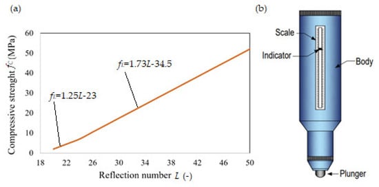
Figure 1.
(a) Base curve according to the standard [13]; and (b) Schmidt hammer.
2.2.2. Pull-Off Tests
Four boreholes were drilled on the prepared panels after each curing time as shown in Figure 2a. The holes were drilled with a 50 mm inside diameter, using diamond saw to a depth of 8 mm. This will clarify the tests directly on the near-surface layer, which was defined as a range from 0 to 4 mm depth (Figure 2b). According to the standard [19], to achieve meaningful results, it was necessary to place the edge of the disc a minimum of 50 mm from the edge of the specimen. After drilling, the surface of the discs was vacuumed and cleaned with acetone without compromising the integrity of the coating. Then, in order to connect the Proceq Dy-216 test device to the specimen, the steel discs (cleaned with acetone) were glued to the wells with Poxipol two-component adhesive. The glue was applied to the surface of the puck and the surface of the sample, then positioning the puck by carefully pressing it to remove air bubbles. The adhesive had no effect on the test specimen. Once the adhesive was fully cured, the test was proceeded. The connection between the puck and the test instrument was screwed into the puck. The machine was levelled and programmed to complete the test in a maximum of 100 s at a loading rate of 0.05 MPa/s. The result of the test is recorded on the instrument along with a graph of load increase over time. After entering the relevant data into the apparatus, the pull-off strength was automatically calculated from Equation (3). Regarding the work of [20] and [21] where the pull-off strength between the substrate layer and the overlay layer is predicted using ANN, the network performed on the basis of the obtained results is supposed to allow for us to estimate the pull-off strength of the near-surface layer as the most exposed layer.
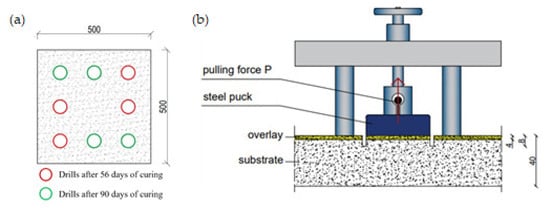
Figure 2.
Pull-off test: (a) pull-off disc arrangement diagram; and (b) pull-off test.
2.2.3. Neural Networks
As we work to reduce the use of cement in the construction of subfloors, replacing it with waste granite powder, it is necessary to determine the optimal values of the components while maintaining the appropriate parameters of the final product. In order to optimize the process of designing the composition of cement mortars with cement replacements, artificial neural networks (ANN) in the form of multilayer perceptron (MLP) were used. MLP is one of the most recognized ANNs used when solving design problems in the construction industry. Karthiyaini et al. [22] predicted the mechanical strength of concrete, doped with fibers, using a multiple regression model (MRA) and an artificial neural network (ANN). The purpose of their work was to compare the two models with each other. The work of Mehdi et al. [23] describes the use of evolutionary neural networks (EANN), as a combination of artificial neural network (ANN) and evolutionary search procedures, in predicting the compressive strength of concrete. Panagiotis G. Asteris et al. [24] trained a database, in conventional machine learning models, of an artificial neural network (ANN) to predict the compressive strength of concrete. Czarnecki et al. [25] presented the application of artificial neural networks (ANNs) to nondestructively evaluate the adhesion of a repair overlay to a concrete substrate. The subject of the paper by Czarnecki et al. [26] was the prediction of the strength of a cementitious composite with the addition of ground granulated blast-furnace slag. There, they compared an artificial neural network (ANN) with a self-organizing feature map (SOFM). This tool is eagerly used by researchers to work with cementitious composites because it can handle inconsistent or “noisy” information which is a common occurrence when studying these materials. According to Figure 3, an artificial neural network in the form of an MLP consists of three layers: input, output, and one or two hidden. Each layer can have one or more neurons. Before interpreting the results, such networks should be subjected to training.
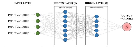
Figure 3.
Block diagram of an artificial neural network.
For the purpose of this study, the MATLAB program was used for designing the neural networks’ structures and learning algorithms as: gradient descent algorithm, conjugate gradient algorithm, and the Broyden–Fletcher–Goldfarb–Shanno and Levenberg–Marquardt algorithms. It also allows the use of 5 types of hidden layer activation functions and output layer activation functions. During ANN modelling, calculations were made for all possible combinations of the above-mentioned network elements. In addition, the number of hidden layer neurons was changed in the range of 1 to 15. We changed the number of layers of hidden neurons to 2 and again edited the number of neurons in layer 1 and layer 2 in the range of 1 to 15. Each of these functions processes the data using the corresponding Formulaes (4)–(8):
Based on the database created, each input variable has 7 parameters, including: (1) the amount of cement (C), (2) the amount of sand (S), (3) the amount of water (W), (4) the amount of granite powder (GP), (5) the curing method (dry or wet), (6) the curing time, and (7) the compressive strength tested with a Schmidt hammer (fc). The output parameter consists of the tensile strength values of the floor mortar substrate measured using pull-off method.
3. Results
3.1. Schmidt Hammer Test
The samples were compared with each other based on the amount of granite powder added to partially replace the cement, as well as based on the maturation conditions of the samples. Figure 4 shows the average compressive strengths obtained when testing each of the sleepers. The basic requirement for cementitious composite substrates in terms of compressive strength is to achieve a minimum value of 20 MPa. It can be seen that all of the samples made reached the minimum value; therefore, the results obtained were used to make a database. From the graph, it can be seen that, as the amount of granite powder in the mix increases, the compressive strength of the substrate decreases, but even for the samples with the highest filler content, the substrate achieved the required strength.
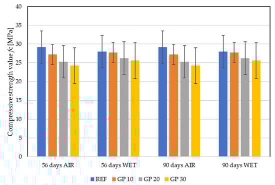
Figure 4.
Average compressive strength of the near-surface layer fc.
3.2. Pull-Off Tests
The samples were compared to each other due to the amount of granite powder added to partially replace the cement, as well as the conditions and maturation time of the samples. Figure 5 shows the average pull-off strengths of each mixture. First of all, it can be seen that there is a large difference in the results due to the different maturation conditions of the samples. Variation in testing time also affected the results. Likewise, the amount of granite powder replacing the cement made a difference. It can be noted that, with the amount of 10% filler, the obtained results for the air-matured samples increased, which suggests the validity of using this modern waste approach to mortar design.

Figure 5.
Average pull-off strength fh of the near-surface layer fc.
4. Statistical Analyses of the Collected Data
The whole dataset is presented in Appendix A. The minimum, maximum, mean, standard deviation, and range of the parameters included in the database are shown in Table 2.
Table 2.
Range of input and output variables.
The correlation coefficients between all possible variables are shown in Table 3. High positive or negative correlation coefficient values between input variables can result in low efficiency and difficulty in determining the impact of these variables on the response. There are no significant correlations between the independent input variables, which was to be expected. As expected, it is clear that there is a strong correlation between the mortar fh and input parameters, such as the amount of cement and granite powder, water-to-cement ratio (W/C), and curing method. In addition, Figure 6 shows the frequency histogram of the six input parameters. These figures are extremely useful because they can help identify the range of parameter values where the data are insufficient and where more data are required.
Table 3.
Correlation matrix of the input and output variables.
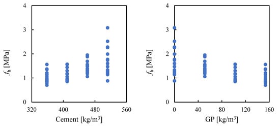
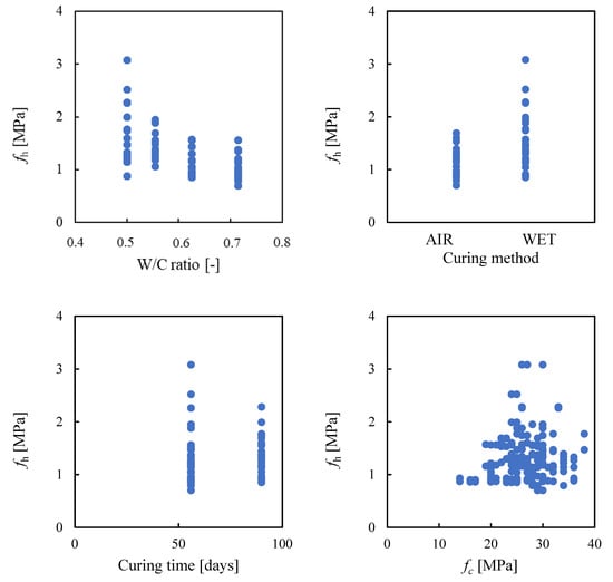
Figure 6.
The relation between input variables and tensile strength.
5. Neural Network Analyses
Using numerical methods of design and prediction, it is necessary to create a database. Based on the results of the study, a database was created containing information on the material composition of the four previously mentioned mortars, how and when they were matured, and the results of the tests presented in Section 2 and Section 3. To meet the requirements of the PN-EN 12504-2 standard of the Schmidt hammer tests, the authors decided to performed the four pull-off tests for each composition and maturing conditions, and, in each of these areas, the three Schmidt hammer tests were performed. Because these three tests inside one pull-off area is less than that stated in the standard, the authors have not calculated the average value out of them. With this, a database of 192 data sets was collected, which were divided into a set for the learning process (136 data sets—70%), the testing process (28 data sets—15%), and the validation process (28 data sets—15%), in a machine-learning model with artificial neural networks (ANN).
Using the ranking method, the most effective artificial neural network was determined, whose calculated values of R2 (9), NRMSE (10), MAE (11), and MAPE (12) were, at the same time, closest to the ideal values of the given indicators.
In the given formulae, is the i-th actual value obtained in the experimental part, while is the i-th value predicted by the network. The total number of data is described by r, and is the average of the real values, i.e., the experimental value of the cement composite.
Figure 7 illustrates the results of the predicted values of the pull-off strength in relation to the results obtained by the experimental method using the gradient descent learning algorithm with one layer of hidden neurons. With this algorithm, the best ability to predict the subsurface tensile strength of cementitious composite containing granite powder was obtained for a network with two hidden-layer neurons. It obtained the following network fit evaluation indices: , , , and Figure 6 shows the results for the learning process (blue rhombuses), the testing process (pink triangles), and the validation process (green circles). The red solid line with the function represents a perfect match, while the dashed lines represent the 20% error area. About 16% of the results are outside this area.
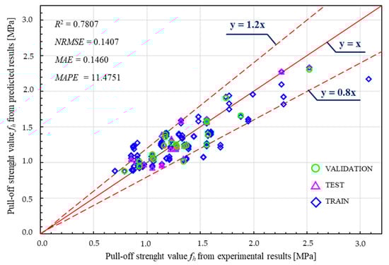
Figure 7.
Relationship between the predicted value and the experimental value of the pull-off strength fh for ANN test, train, and validation process for the GD algorithm with one layer of hidden neurons.
Figure 8 illustrates the results of the predicted values of the pull-off strength in relation to the results obtained by the experimental method using the Broyden–Fletcher–Goldfarb–Shanno learning algorithm with one layer of hidden neurons. With this algorithm, the best ability to predict the subsurface tensile strength of cementitious composite containing granite powder was obtained for a network with nine hidden-layer neurons. It obtained the following network fit evaluation indices: , , , and Figure 7 shows the results for the learning process (blue rhombuses), the testing process (pink triangles), and the validation process (green circles). The red solid line with the function represents a perfect match while the dashed lines represent the 20% error area. About 6% of the results are outside this area.
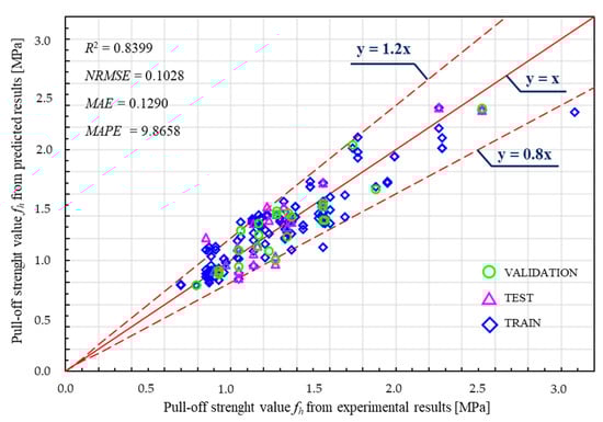
Figure 8.
Relationship between the predicted value and the experimental value of the pull-off strength fh for ANN test, train, and validation process for the BFGS algorithm with one layer of hidden neurons.
Figure 9 illustrates the results of the predicted values of the pull-off strength in relation to the results obtained by the experimental method using the Levenberg–Marquardt learning algorithm with one layer of hidden neurons. With this algorithm, the best ability to predict the subsurface tensile strength of cementitious composite containing granite powder was obtained for a network with seven hidden-layer neurons. It obtained the following network fit evaluation indices: , , , and Figure 8 shows the results for the learning process (blue rhombuses), the testing process (pink triangles), and the validation process (green circles). The red solid line with the function represents a perfect match while the dashed lines represent the 20% error area. About 9% of the results are outside this area.
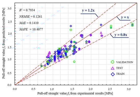
Figure 9.
Relationship between the predicted value and the experimental value of the pull-off strength fh for ANN test, train, and validation process for the LM algorithm with one layer of hidden neurons.
Figure 10 illustrates the results of the predicted values of the pull-off strength in relation to the results obtained by the experimental method using the conjugate gradient learning algorithm with one layer of hidden neurons. With this algorithm, the best ability to predict the subsurface tensile strength of cementitious composite containing granite powder was obtained for a network with three hidden-layer neurons. It obtained the following network fit evaluation indices: , , , and Figure 9 shows the results for the learning process (blue rhombuses), the testing process (pink triangles), and the validation process (green circles). The red solid line with the function represents a perfect match while the dashed lines represent the 20% error area. About 10% of the results are outside this area.
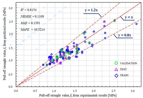
Figure 10.
Relationship between the predicted value and the experimental value of the pull-off strength fh for ANN test, train, and validation process for the CG algorithm with one layer of hidden neurons.
Figure 11 illustrates the results of the predicted values of the pull-off strength in relation to the results obtained by the experimental method using the gradient descent learning algorithm with two layers of hidden neurons. With this algorithm, the best ability to predict the subsurface tensile strength of cementitious composite containing granite powder was obtained for a network with 13 neurons in the first hidden layer and 15 neurons in the second hidden layer. It obtained the following network fit evaluation indices: , , , and Figure 10 shows the results for the learning process (blue rhombuses), the testing process (pink triangles), and the validation process (green circles). The red solid line with the function represents a perfect match while the dashed lines represent the 20% error area. About 18% of the results are outside this area.
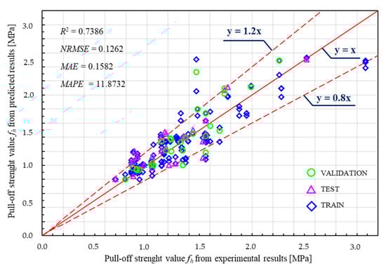
Figure 11.
Relationship between the predicted value and the experimental value of the pull-off strength fh for ANN test, train, and validation process for the GD algorithm with two layers of hidden neurons.
Figure 12 illustrates the results of the predicted values of the pull-off strength in relation to the results obtained by the experimental method using the Broyden–Fletcher–Goldfarb–Shanno learning algorithm with two layers of hidden neurons. With this algorithm, the best ability to predict the subsurface tensile strength of cementitious composite containing granite powder was obtained for a network with four neurons in the first hidden layer and three neurons in the second hidden layer. It obtained the following network fit evaluation indices: , , , and Figure 11 shows the results for the learning process (blue rhombuses), the testing process (pink triangles), and the validation process (green circles). The red solid line with the function represents a perfect match while the dashed lines represent the 20% error area. About 11.5% of the results are outside this area.
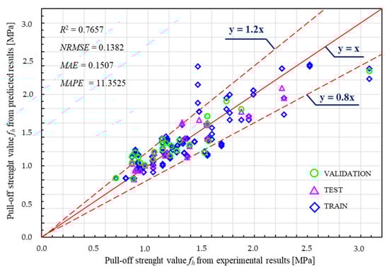
Figure 12.
Relationship between the predicted value and the experimental value of the pull-off strength fh for ANN test, train, and validation process for the BFGS algorithm with two layers of hidden neurons.
Figure 13 illustrates the results of the predicted values of the pull-off strength in relation to the results obtained by the experimental method using the Levenberg–Marquardt learning algorithm with two layers of hidden neurons. With this algorithm, the best ability to predict the subsurface tensile strength of cementitious composite containing granite powder was obtained for a network with four neurons in the first hidden layer and 10 neurons in the second hidden layer. It obtained the following network fit evaluation indices: , , , and Figure 12 shows the results for the learning process (blue rhombuses), the testing process (pink triangles), and the validation process (green circles). The red solid line with the function represents a perfect match while the dashed lines represent the 20% error area. About 8% of the results are outside this area.
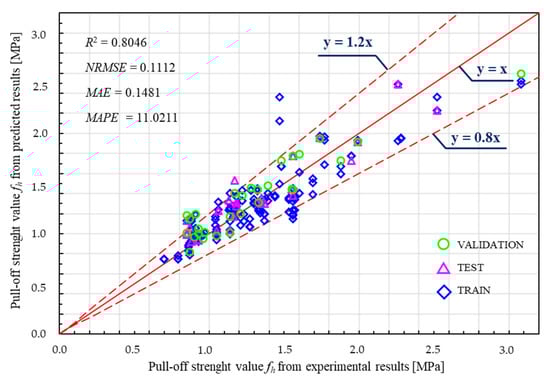
Figure 13.
Relationship between the predicted value and the experimental value of the pull-off strength fh for ANN test, train, and validation process for the LM algorithm with two layers of hidden neurons.
Figure 14 illustrates the results of the predicted values of the pull-off strength in relation to the results obtained by the experimental method using the conjugate gradient learning algorithm with two layers of hidden neurons. With this algorithm, the best ability to predict the subsurface tensile strength of cementitious composite containing granite powder was obtained for a network with 11 neurons in the first hidden layer and eight neurons in the second hidden layer. It obtained the following network fit evaluation indices: , , , and Figure 13 shows the results for the learning process (blue rhombuses), the testing process (pink triangles), and the validation process (green circles). The red solid line with the function represents a perfect match while the dashed lines represent the 20% error area. About 11% of the results are outside this area.
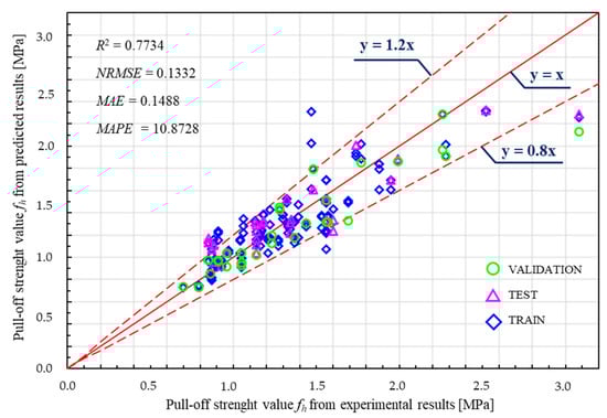
Figure 14.
Relationship between the predicted value and the experimental value of the pull-off strength fh for ANN test, train, and validation process for the CG algorithm with two layers of hidden neurons.
6. Comparison of the Models
The network allows us to estimate the strength based on the material composition of the floor mortar and the compressive strength value determined by the Schmidt hammer. This allows the use of a nondestructive method to evaluate the peel strength, thereby not exposing the tested surface to the repairs necessary after using the pull-off method. Subsequently, using the Schmidt hammer, it is possible to obtain both the compressive strength and pull-off strength. These are the two most important characteristics of floor substrates.
The machine-learning algorithms used in the article are accurate in predicting the subsurface tensile strength of green cementitious composites. This can be concluded from the values of the parameters determining their accuracy, which were R2, NRMSE, MAE, and MAPE. Figure 15, Figure 16, Figure 17, Figure 18 and Figure 19 and Table 4 compare the above algorithms. It can be seen that all the models tested predict the tensile strength of green cement composites well. The BFGS algorithm with one layer of hidden neurons performed best. However, since none of the models were perfectly accurate (R2 would be equal to 1; and NRMSE, MAE, MAPE, and relative error would be equal to 0), there is still room for improvement in the algorithms by building other databases or using other algorithms.
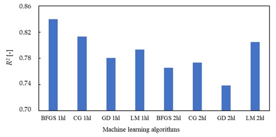
Figure 15.
Comparison of models for predicting the pull-off strength of the surface layer fh due to the value of R2.
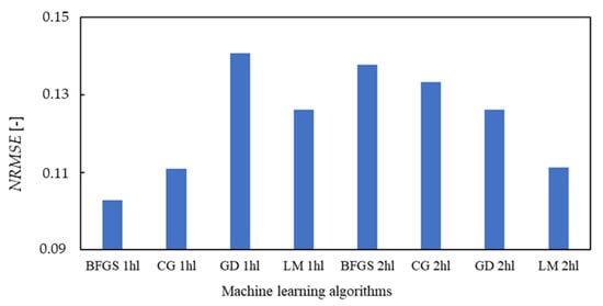
Figure 16.
Comparison of models for predicting the pull-off strength of the surface layer fh due to the value of NRMSE.
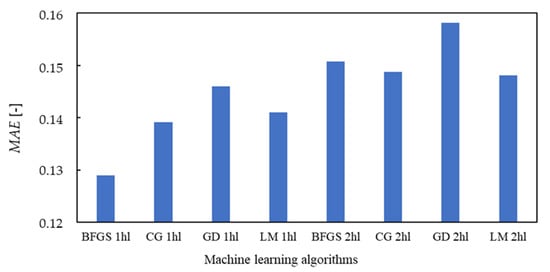
Figure 17.
Comparison of models for predicting the pull-off strength of the surface layer fh due to the value of MAE.
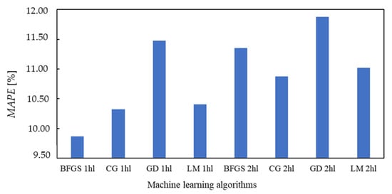
Figure 18.
Comparison of models for predicting the pull-off strength of the surface layer fh due to the value of MAPE.
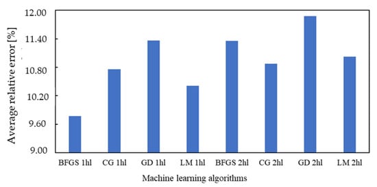
Figure 19.
Comparison of models for predicting the pull-off strength of the surface layer fh due to the value of average relative error.
Table 4.
Comparison of accuracy of compared neural networks.
The network based on the BFGS algorithm with nine hidden-layer neurons performed best in predicting the pull-off strength of cement floor underlayments. It obtained the following network fit evaluation indices: , , , and . According to the article [10], the values of determination coefficients achieved by the selected network are within the range of a very good match with the results obtained experimentally because . The MAPE absolute percentage error values of up to 10% are defined as a good fit. As can be seen in Figure 6, the presented network correctly predicts the pull-off strength of the surface layer. The strength ranging from 0.8 MPa to 2.6 MPa is predicted with similar accuracy. The result obtained for the experimental strength above 3 MPa significantly deviates from the rest of the results. This may be due to insufficient batch data from the 2.8 MPa to 3.2 MPa range. It should be noted that the prediction accuracy in the learning, testing, and validation processes of the given network was similar.
7. Conclusions
In this work, the authors proposed a hybrid neural–nondestructive model of subsurface tensile strength prediction in cementitious composites containing granite powder. For this purpose, the experimental tests using a Schmidt hammer were performed, combined with numerical analyses using neural networks. It has been proven that it is possible to design such accurate models using a neural network with the Broyden–Fletcher–Goldfarb–Shanno learning algorithm. The performance was very good, which was shown by the very high value of the coefficient of determination R2, equal to 0.8399, and very low values of the errors presented as NRMSE, MAE, and MAPE, equal to 0.1028, 0.1290, and 9.8658%, respectively. According to the results of the correlation between the input variables and output parameter, it can be seen that the amount of cement content and curing conditions contributed the most to the output parameter, whether the samples were kept in a dry environment or wet.
One of the advantages of this method is the fact that it can be used in existing structures, without a need to obtain the samples and destroy them. Moreover, it can still be used after almost 100 days of concreting. Because different curing conditions were taken into account, this method is more universal in comparison to standardized equations.
This novel approach can be a reasonable alternative for evaluating the properties of spacious mortar elements in which there is a need to analyse not only the compressive strength but also its subsurface tensile strength. Moreover, it is worth emphasizing that using a Schmidt hammer during the tests allows us to evaluate the compressive strength, which is beneficial in order to shorten the time of analysing the cementitious composite element.
However, there are some limitations which should be considered before using it in practice. Firstly, it has not been tested yet in the field; therefore, there is need for experimental verification. Second, it has not been used to evaluate the subsurface tensile strength of composites containing admixtures other than granite powder, which might be interesting from a cognitive point of view. Moreover, even though the mortars have been tested, there is still an open question if this model is suitable for concrete containing core aggregates.
Taking the above into account, the authors are still investigating the possibility of using these methods for different cementitious composite mixtures containing such admixtures as fly ash and blast-furnace slag. Moreover, the authors are trying different algorithms such as SVM, linear regression, or random forest, which might be more accurate than those presented in the article. Because this is still an open problem, the authors submit the data to the article for other researchers to use.
Author Contributions
Conceptualization, S.C. and M.M.; methodology, S.C.; software, S.C. and M.M.; validation, S.C.; formal analysis, S.C. and M.M.; investigation, S.C. and M.M.; resources, S.C. and M.M.; data curation, S.C. and M.M.; writing—original draft preparation, S.C. and M.M.; writing—review and editing, S.C.; visualization, M.M.; supervision, S.C.; project administration, S.C.; funding acquisition, S.C. All authors have read and agreed to the published version of the manuscript.
Funding
The authors received funding for preparing the samples from the project, supported by the National Centre for Research and Development, Poland [grant no. LIDER/35/0130/L-11/19/NCBR/2020 “The use of granite powder waste for the production of selected construction products.”].
Institutional Review Board Statement
Not applicable.
Informed Consent Statement
Not applicable.
Data Availability Statement
Data available upon request.
Conflicts of Interest
The authors declare no conflict of interest.
Appendix A
Table A1.
Data collected during studies.
Table A1.
Data collected during studies.
| Sample No. | Cement [kg/m3] | Dry Quartz Sand [kg/m3] | Water [kg/m3] | Granite Powder [kg/m3] | Curing Conditions | Curing Time [days] | fc [MPa] | fh [MPa] |
|---|---|---|---|---|---|---|---|---|
| 1 | 512 | 1536 | 256 | 0 | AIR | 56 | 22 | 1.23 |
| 2 | 512 | 1536 | 256 | 0 | AIR | 56 | 24 | 1.23 |
| 3 | 512 | 1536 | 256 | 0 | AIR | 56 | 27 | 1.23 |
| 4 | 512 | 1536 | 256 | 0 | AIR | 56 | 29 | 1.27 |
| 5 | 512 | 1536 | 256 | 0 | AIR | 56 | 34 | 1.27 |
| 6 | 512 | 1536 | 256 | 0 | AIR | 56 | 36 | 1.27 |
| 7 | 512 | 1536 | 256 | 0 | AIR | 56 | 32 | 1.14 |
| 8 | 512 | 1536 | 256 | 0 | AIR | 56 | 27 | 1.14 |
| 9 | 512 | 1536 | 256 | 0 | AIR | 56 | 25 | 1.14 |
| 10 | 512 | 1536 | 256 | 0 | AIR | 56 | 31 | 0.88 |
| 11 | 512 | 1536 | 256 | 0 | AIR | 56 | 36 | 0.88 |
| 12 | 512 | 1536 | 256 | 0 | AIR | 56 | 27 | 0.88 |
| 13 | 460.8 | 1536 | 256 | 51.2 | AIR | 56 | 25 | 1.18 |
| 14 | 460.8 | 1536 | 256 | 51.2 | AIR | 56 | 26 | 1.18 |
| 15 | 460.8 | 1536 | 256 | 51.2 | AIR | 56 | 26 | 1.18 |
| 16 | 460.8 | 1536 | 256 | 51.2 | AIR | 56 | 23 | 1.53 |
| 17 | 460.8 | 1536 | 256 | 51.2 | AIR | 56 | 29 | 1.53 |
| 18 | 460.8 | 1536 | 256 | 51.2 | AIR | 56 | 22 | 1.53 |
| 19 | 460.8 | 1536 | 256 | 51.2 | AIR | 56 | 24 | 1.06 |
| 20 | 460.8 | 1536 | 256 | 51.2 | AIR | 56 | 28 | 1.06 |
| 21 | 460.8 | 1536 | 256 | 51.2 | AIR | 56 | 34 | 1.06 |
| 22 | 460.8 | 1536 | 256 | 51.2 | AIR | 56 | 30 | 1.34 |
| 23 | 460.8 | 1536 | 256 | 51.2 | AIR | 56 | 34 | 1.34 |
| 24 | 460.8 | 1536 | 256 | 51.2 | AIR | 56 | 26 | 1.34 |
| 25 | 409.6 | 1536 | 256 | 102.4 | AIR | 56 | 23 | 0.88 |
| 26 | 409.6 | 1536 | 256 | 102.4 | AIR | 56 | 24 | 0.88 |
| 27 | 409.6 | 1536 | 256 | 102.4 | AIR | 56 | 25 | 0.88 |
| 28 | 409.6 | 1536 | 256 | 102.4 | AIR | 56 | 32 | 1.05 |
| 29 | 409.6 | 1536 | 256 | 102.4 | AIR | 56 | 20 | 1.05 |
| 30 | 409.6 | 1536 | 256 | 102.4 | AIR | 56 | 27 | 1.05 |
| 31 | 409.6 | 1536 | 256 | 102.4 | AIR | 56 | 28 | 0.96 |
| 32 | 409.6 | 1536 | 256 | 102.4 | AIR | 56 | 20 | 0.96 |
| 33 | 409.6 | 1536 | 256 | 102.4 | AIR | 56 | 20 | 0.96 |
| 34 | 409.6 | 1536 | 256 | 102.4 | AIR | 56 | 23 | 0.93 |
| 35 | 409.6 | 1536 | 256 | 102.4 | AIR | 56 | 25 | 0.93 |
| 36 | 409.6 | 1536 | 256 | 102.4 | AIR | 56 | 36 | 0.93 |
| 37 | 358.4 | 1536 | 256 | 153.6 | AIR | 56 | 21 | 0.87 |
| 38 | 358.4 | 1536 | 256 | 153.6 | AIR | 56 | 23 | 0.87 |
| 39 | 358.4 | 1536 | 256 | 153.6 | AIR | 56 | 14 | 0.87 |
| 40 | 358.4 | 1536 | 256 | 153.6 | AIR | 56 | 20 | 0.86 |
| 41 | 358.4 | 1536 | 256 | 153.6 | AIR | 56 | 17 | 0.86 |
| 42 | 358.4 | 1536 | 256 | 153.6 | AIR | 56 | 16 | 0.86 |
| 43 | 358.4 | 1536 | 256 | 153.6 | AIR | 56 | 30 | 0.7 |
| 44 | 358.4 | 1536 | 256 | 153.6 | AIR | 56 | 29 | 0.7 |
| 45 | 358.4 | 1536 | 256 | 153.6 | AIR | 56 | 30 | 0.7 |
| 46 | 358.4 | 1536 | 256 | 153.6 | AIR | 56 | 34 | 0.79 |
| 47 | 358.4 | 1536 | 256 | 153.6 | AIR | 56 | 29 | 0.79 |
| 48 | 358.4 | 1536 | 256 | 153.6 | AIR | 56 | 28 | 0.79 |
| 49 | 512 | 1536 | 256 | 0 | WET | 56 | 24 | 2.52 |
| 50 | 512 | 1536 | 256 | 0 | WET | 56 | 24 | 2.52 |
| 51 | 512 | 1536 | 256 | 0 | WET | 56 | 25 | 2.52 |
| 52 | 512 | 1536 | 256 | 0 | WET | 56 | 26 | 2.26 |
| 53 | 512 | 1536 | 256 | 0 | WET | 56 | 26 | 2.26 |
| 54 | 512 | 1536 | 256 | 0 | WET | 56 | 33 | 2.26 |
| 55 | 512 | 1536 | 256 | 0 | WET | 56 | 38 | 1.47 |
| 56 | 512 | 1536 | 256 | 0 | WET | 56 | 32 | 1.47 |
| 57 | 512 | 1536 | 256 | 0 | WET | 56 | 25 | 1.47 |
| 58 | 512 | 1536 | 256 | 0 | WET | 56 | 27 | 3.08 |
| 59 | 512 | 1536 | 256 | 0 | WET | 56 | 30 | 3.08 |
| 60 | 512 | 1536 | 256 | 0 | WET | 56 | 26 | 3.08 |
| 61 | 460.8 | 1536 | 256 | 51.2 | WET | 56 | 26 | 1.48 |
| 62 | 460.8 | 1536 | 256 | 51.2 | WET | 56 | 30 | 1.48 |
| 63 | 460.8 | 1536 | 256 | 51.2 | WET | 56 | 26 | 1.48 |
| 64 | 460.8 | 1536 | 256 | 51.2 | WET | 56 | 25 | 1.88 |
| 65 | 460.8 | 1536 | 256 | 51.2 | WET | 56 | 26 | 1.88 |
| 66 | 460.8 | 1536 | 256 | 51.2 | WET | 56 | 30 | 1.88 |
| 67 | 460.8 | 1536 | 256 | 51.2 | WET | 56 | 30 | 1.95 |
| 68 | 460.8 | 1536 | 256 | 51.2 | WET | 56 | 28 | 1.95 |
| 69 | 460.8 | 1536 | 256 | 51.2 | WET | 56 | 28 | 1.95 |
| 70 | 460.8 | 1536 | 256 | 51.2 | WET | 56 | 28 | 1.56 |
| 71 | 460.8 | 1536 | 256 | 51.2 | WET | 56 | 28 | 1.56 |
| 72 | 460.8 | 1536 | 256 | 51.2 | WET | 56 | 28 | 1.56 |
| 73 | 409.6 | 1536 | 256 | 102.4 | WET | 56 | 19 | 1.16 |
| 74 | 409.6 | 1536 | 256 | 102.4 | WET | 56 | 26 | 1.16 |
| 75 | 409.6 | 1536 | 256 | 102.4 | WET | 56 | 29 | 1.16 |
| 76 | 409.6 | 1536 | 256 | 102.4 | WET | 56 | 23 | 0.91 |
| 77 | 409.6 | 1536 | 256 | 102.4 | WET | 56 | 24 | 0.91 |
| 78 | 409.6 | 1536 | 256 | 102.4 | WET | 56 | 27 | 0.91 |
| 79 | 409.6 | 1536 | 256 | 102.4 | WET | 56 | 21 | 1.56 |
| 80 | 409.6 | 1536 | 256 | 102.4 | WET | 56 | 24 | 1.56 |
| 81 | 409.6 | 1536 | 256 | 102.4 | WET | 56 | 30 | 1.56 |
| 82 | 409.6 | 1536 | 256 | 102.4 | WET | 56 | 32 | 0.87 |
| 83 | 409.6 | 1536 | 256 | 102.4 | WET | 56 | 30 | 0.87 |
| 84 | 409.6 | 1536 | 256 | 102.4 | WET | 56 | 30 | 0.87 |
| 85 | 358.4 | 1536 | 256 | 153.6 | WET | 56 | 24 | 0.85 |
| 86 | 358.4 | 1536 | 256 | 153.6 | WET | 56 | 28 | 0.85 |
| 87 | 358.4 | 1536 | 256 | 153.6 | WET | 56 | 24 | 0.85 |
| 88 | 358.4 | 1536 | 256 | 153.6 | WET | 56 | 30 | 1.37 |
| 89 | 358.4 | 1536 | 256 | 153.6 | WET | 56 | 29 | 1.37 |
| 90 | 358.4 | 1536 | 256 | 153.6 | WET | 56 | 24 | 1.37 |
| 91 | 358.4 | 1536 | 256 | 153.6 | WET | 56 | 25 | 1.04 |
| 92 | 358.4 | 1536 | 256 | 153.6 | WET | 56 | 20 | 1.04 |
| 93 | 358.4 | 1536 | 256 | 153.6 | WET | 56 | 27 | 1.04 |
| 94 | 358.4 | 1536 | 256 | 153.6 | WET | 56 | 20 | 1.21 |
| 95 | 358.4 | 1536 | 256 | 153.6 | WET | 56 | 30 | 1.21 |
| 96 | 358.4 | 1536 | 256 | 153.6 | WET | 56 | 26 | 1.21 |
| 97 | 512 | 1536 | 256 | 0 | AIR | 90 | 22 | 1.6 |
| 98 | 512 | 1536 | 256 | 0 | AIR | 90 | 24 | 1.6 |
| 99 | 512 | 1536 | 256 | 0 | AIR | 90 | 27 | 1.6 |
| 100 | 512 | 1536 | 256 | 0 | AIR | 90 | 29 | 1.33 |
| 101 | 512 | 1536 | 256 | 0 | AIR | 90 | 34 | 1.33 |
| 102 | 512 | 1536 | 256 | 0 | AIR | 90 | 36 | 1.33 |
| 103 | 512 | 1536 | 256 | 0 | AIR | 90 | 32 | 1.17 |
| 104 | 512 | 1536 | 256 | 0 | AIR | 90 | 27 | 1.17 |
| 105 | 512 | 1536 | 256 | 0 | AIR | 90 | 25 | 1.17 |
| 106 | 512 | 1536 | 256 | 0 | AIR | 90 | 31 | 1.14 |
| 107 | 512 | 1536 | 256 | 0 | AIR | 90 | 36 | 1.14 |
| 108 | 512 | 1536 | 256 | 0 | AIR | 90 | 27 | 1.14 |
| 109 | 460.8 | 1536 | 256 | 51.2 | AIR | 90 | 25 | 1.28 |
| 110 | 460.8 | 1536 | 256 | 51.2 | AIR | 90 | 26 | 1.28 |
| 111 | 460.8 | 1536 | 256 | 51.2 | AIR | 90 | 26 | 1.28 |
| 112 | 460.8 | 1536 | 256 | 51.2 | AIR | 90 | 23 | 1.69 |
| 113 | 460.8 | 1536 | 256 | 51.2 | AIR | 90 | 29 | 1.69 |
| 114 | 460.8 | 1536 | 256 | 51.2 | AIR | 90 | 22 | 1.69 |
| 115 | 460.8 | 1536 | 256 | 51.2 | AIR | 90 | 24 | 1.39 |
| 116 | 460.8 | 1536 | 256 | 51.2 | AIR | 90 | 28 | 1.39 |
| 117 | 460.8 | 1536 | 256 | 51.2 | AIR | 90 | 34 | 1.39 |
| 118 | 460.8 | 1536 | 256 | 51.2 | AIR | 90 | 30 | 1.22 |
| 119 | 460.8 | 1536 | 256 | 51.2 | AIR | 90 | 34 | 1.22 |
| 120 | 460.8 | 1536 | 256 | 51.2 | AIR | 90 | 26 | 1.22 |
| 121 | 409.6 | 1536 | 256 | 102.4 | AIR | 90 | 23 | 0.85 |
| 122 | 409.6 | 1536 | 256 | 102.4 | AIR | 90 | 24 | 0.85 |
| 123 | 409.6 | 1536 | 256 | 102.4 | AIR | 90 | 25 | 0.85 |
| 124 | 409.6 | 1536 | 256 | 102.4 | AIR | 90 | 32 | 1.05 |
| 125 | 409.6 | 1536 | 256 | 102.4 | AIR | 90 | 20 | 1.05 |
| 126 | 409.6 | 1536 | 256 | 102.4 | AIR | 90 | 27 | 1.05 |
| 127 | 409.6 | 1536 | 256 | 102.4 | AIR | 90 | 28 | 1.05 |
| 128 | 409.6 | 1536 | 256 | 102.4 | AIR | 90 | 20 | 1.05 |
| 129 | 409.6 | 1536 | 256 | 102.4 | AIR | 90 | 20 | 1.05 |
| 130 | 409.6 | 1536 | 256 | 102.4 | AIR | 90 | 23 | 0.91 |
| 131 | 409.6 | 1536 | 256 | 102.4 | AIR | 90 | 25 | 0.91 |
| 132 | 409.6 | 1536 | 256 | 102.4 | AIR | 90 | 36 | 0.91 |
| 133 | 358.4 | 1536 | 256 | 153.6 | AIR | 90 | 21 | 0.93 |
| 134 | 358.4 | 1536 | 256 | 153.6 | AIR | 90 | 23 | 0.93 |
| 135 | 358.4 | 1536 | 256 | 153.6 | AIR | 90 | 14 | 0.93 |
| 136 | 358.4 | 1536 | 256 | 153.6 | AIR | 90 | 20 | 0.9 |
| 137 | 358.4 | 1536 | 256 | 153.6 | AIR | 90 | 17 | 0.9 |
| 138 | 358.4 | 1536 | 256 | 153.6 | AIR | 90 | 16 | 0.9 |
| 139 | 358.4 | 1536 | 256 | 153.6 | AIR | 90 | 30 | 0.97 |
| 140 | 358.4 | 1536 | 256 | 153.6 | AIR | 90 | 29 | 0.97 |
| 141 | 358.4 | 1536 | 256 | 153.6 | AIR | 90 | 30 | 0.97 |
| 142 | 358.4 | 1536 | 256 | 153.6 | AIR | 90 | 34 | 1.14 |
| 143 | 358.4 | 1536 | 256 | 153.6 | AIR | 90 | 29 | 1.14 |
| 144 | 358.4 | 1536 | 256 | 153.6 | AIR | 90 | 28 | 1.14 |
| 145 | 512 | 1536 | 256 | 0 | WET | 90 | 24 | 1.99 |
| 146 | 512 | 1536 | 256 | 0 | WET | 90 | 24 | 1.99 |
| 147 | 512 | 1536 | 256 | 0 | WET | 90 | 25 | 1.99 |
| 148 | 512 | 1536 | 256 | 0 | WET | 90 | 26 | 2.28 |
| 149 | 512 | 1536 | 256 | 0 | WET | 90 | 26 | 2.28 |
| 150 | 512 | 1536 | 256 | 0 | WET | 90 | 33 | 2.28 |
| 151 | 512 | 1536 | 256 | 0 | WET | 90 | 38 | 1.77 |
| 152 | 512 | 1536 | 256 | 0 | WET | 90 | 32 | 1.77 |
| 153 | 512 | 1536 | 256 | 0 | WET | 90 | 25 | 1.77 |
| 154 | 512 | 1536 | 256 | 0 | WET | 90 | 27 | 1.74 |
| 155 | 512 | 1536 | 256 | 0 | WET | 90 | 30 | 1.74 |
| 156 | 512 | 1536 | 256 | 0 | WET | 90 | 26 | 1.74 |
| 157 | 460.8 | 1536 | 256 | 51.2 | WET | 90 | 26 | 1.56 |
| 158 | 460.8 | 1536 | 256 | 51.2 | WET | 90 | 30 | 1.56 |
| 159 | 460.8 | 1536 | 256 | 51.2 | WET | 90 | 26 | 1.56 |
| 160 | 460.8 | 1536 | 256 | 51.2 | WET | 90 | 25 | 1.32 |
| 161 | 460.8 | 1536 | 256 | 51.2 | WET | 90 | 26 | 1.32 |
| 162 | 460.8 | 1536 | 256 | 51.2 | WET | 90 | 30 | 1.32 |
| 163 | 460.8 | 1536 | 256 | 51.2 | WET | 90 | 30 | 1.56 |
| 164 | 460.8 | 1536 | 256 | 51.2 | WET | 90 | 28 | 1.56 |
| 165 | 460.8 | 1536 | 256 | 51.2 | WET | 90 | 28 | 1.56 |
| 166 | 460.8 | 1536 | 256 | 51.2 | WET | 90 | 28 | 1.55 |
| 167 | 460.8 | 1536 | 256 | 51.2 | WET | 90 | 28 | 1.55 |
| 168 | 460.8 | 1536 | 256 | 51.2 | WET | 90 | 28 | 1.55 |
| 169 | 409.6 | 1536 | 256 | 102.4 | WET | 90 | 19 | 1.57 |
| 170 | 409.6 | 1536 | 256 | 102.4 | WET | 90 | 26 | 1.57 |
| 171 | 409.6 | 1536 | 256 | 102.4 | WET | 90 | 29 | 1.57 |
| 172 | 409.6 | 1536 | 256 | 102.4 | WET | 90 | 23 | 1.3 |
| 173 | 409.6 | 1536 | 256 | 102.4 | WET | 90 | 24 | 1.3 |
| 174 | 409.6 | 1536 | 256 | 102.4 | WET | 90 | 27 | 1.3 |
| 175 | 409.6 | 1536 | 256 | 102.4 | WET | 90 | 21 | 1.18 |
| 176 | 409.6 | 1536 | 256 | 102.4 | WET | 90 | 24 | 1.18 |
| 177 | 409.6 | 1536 | 256 | 102.4 | WET | 90 | 30 | 1.18 |
| 178 | 409.6 | 1536 | 256 | 102.4 | WET | 90 | 32 | 1.44 |
| 179 | 409.6 | 1536 | 256 | 102.4 | WET | 90 | 30 | 1.44 |
| 180 | 409.6 | 1536 | 256 | 102.4 | WET | 90 | 30 | 1.44 |
| 181 | 358.4 | 1536 | 256 | 153.6 | WET | 90 | 24 | 1.37 |
| 182 | 358.4 | 1536 | 256 | 153.6 | WET | 90 | 28 | 1.37 |
| 183 | 358.4 | 1536 | 256 | 153.6 | WET | 90 | 24 | 1.37 |
| 184 | 358.4 | 1536 | 256 | 153.6 | WET | 90 | 30 | 1.35 |
| 185 | 358.4 | 1536 | 256 | 153.6 | WET | 90 | 29 | 1.35 |
| 186 | 358.4 | 1536 | 256 | 153.6 | WET | 90 | 24 | 1.35 |
| 187 | 358.4 | 1536 | 256 | 153.6 | WET | 90 | 25 | 1.13 |
| 188 | 358.4 | 1536 | 256 | 153.6 | WET | 90 | 20 | 1.13 |
| 189 | 358.4 | 1536 | 256 | 153.6 | WET | 90 | 27 | 1.13 |
| 190 | 358.4 | 1536 | 256 | 153.6 | WET | 90 | 20 | 1.56 |
| 191 | 358.4 | 1536 | 256 | 153.6 | WET | 90 | 30 | 1.56 |
| 192 | 358.4 | 1536 | 256 | 153.6 | WET | 90 | 26 | 1.56 |
References
- Danish, A.; Ozbakkaloglu, T. Greener cementitious composites incorporating sewage sludge ash as cement replacement: A review of progress, potentials, and future prospects. J. Clean. Prod. 2022, 371, 133364. [Google Scholar] [CrossRef]
- Nadim Hasoun, M.; Al-Manaseer, A. Structural Concrete: Theory and Design, 7th ed.; Wiley: Hoboken, NJ, USA, 2020; ISBN 978-1-119-60512-6. [Google Scholar]
- Herath, C.; Gunasekara, C.; Law, D.W.; Setunge, S. Performance of high volume fly ash concrete incorporating additives: A systematic literature review. Constr. Build. Mater. 2020, 258, 120606. [Google Scholar] [CrossRef]
- Czarnecki, S. Modelling of Mechanical Properties of Eco-Friendly Cementitious Composites Used in Floors: State of the Art and Research Gaps. Chem. Eng. Trans. 2022, 94, 403–408. [Google Scholar]
- Chajec, A.; Chowaniec, A.; Królicka, A.; Sadowski, Ł.; Żak, A.; Piechowka-Mielnik, M.; Savija, B. Engineering of green cementitious composites modified with siliceous fly ash: Understanding the importance of curing conditions. Constr. Build. Mater. 2021, 313, 125209. [Google Scholar] [CrossRef]
- Chajec, A. Towards the Cleaner Production of Cementitious Materials with the Synergistic Addition of Granite Powder Waste and Fly Ash. Chem. Eng. Trans. 2022, 94, 289–294. [Google Scholar]
- Malla, P.; Khedmatgozar Dolati, S.S.; Ortiz, J.D.; Mehrabi, A.B.; Nanni, A.; Dinh, K. Feasibility of Conventional Non-Destructive Testing Methods in Detecting Embedded FRP Reinforcements. Appl. Sci. 2023, 13, 4399. [Google Scholar] [CrossRef]
- Łątka, D. Prediction of Mortar Compressive Strength Based on Modern Minor-Destructive Tests. Materials 2023, 16, 2402. [Google Scholar] [CrossRef] [PubMed]
- Kazemi, M.; Madandoust, R.; De Brito, J. Compressive strength assessment of recycled aggregate concrete using Schmidt rebound hammer and core testing. Constr. Build. Mater. 2019, 224, 630–638. [Google Scholar] [CrossRef]
- ASTM, C805; Standard Test Method for Rebound Number of Hardened Concrete. ASTM International: West Conshohocken, PA, USA, 2019.
- Cacciari, P.P.; Futai, M.M. Assessing the tensile strength of rocks and geological discontinuities via pull-off tests. Int. J. Rock Mech. Min. Sci. 2018, 105, 44–52. [Google Scholar] [CrossRef]
- Pereira, E.; De Mereiros, M.H.F. Pull Off test to evaluate the compressive strength of concrete: An alternative to Brazilian standard techniques. Ibracon Struct. Mater. J. 2021, 5, 757–780. [Google Scholar] [CrossRef]
- Kos, Ž.; Kroviakov, S.; Kryzhanovskyi, V.; Hedulian, D. Strength, Frost Resistance, and Resistance to Acid Attacks on Fiber-Reinforced Concrete for Industrial Floors and Road Pavements with Steel and Polypropylene Fibers. Materials 2022, 15, 8339. [Google Scholar] [CrossRef]
- Martini, R.; Carvalho, J.; Arede, A.; Varum, H. Validation of nondestructive methods for assessing stone masonry using artificial neural networks. J. Build. Eng. 2021, 42, 102469. [Google Scholar] [CrossRef]
- Le, T.-T.; Skentou, A.D.; Mamou, A.; Asteris, P.G. Correlating the Unconfined Compressive Strength of Rock with the Compressional Wave Velocity Effective Porosity and Schmidt Hammer Rebound Number Using Artificial Neural Networks. Rock Mech. Rock Eng. 2022, 55, 6805–6840. [Google Scholar] [CrossRef]
- Almasaeid, H.H.; Suleiman, A.; Alawneh, R. Assessment of high-temperature damaged concrete using non-destructive tests and artificial neural network modelling. Case Stud. Constr. Mater. 2022, 16, e01080. [Google Scholar] [CrossRef]
- Saleem, M. Assessing the load carrying capacity of concrete anchor bolts using non-destructive tests and artificial multilayer neural network. J. Build. Eng. 2020, 30, 101260. [Google Scholar] [CrossRef]
- PN-EN 12504-2; Testing of Concrete in Structures—Part 2: Non-Destructive Testing—Determination of Reflection Number. Polish Committee for Standardization: Warsaw, Poland, 2021.
- ASTM, D 4541; Standard Test Method for Pull-Off Strength of Coatings Using Portable Adhesion Testers. ASTM International: West Conshohocken, PA, USA, 2017.
- Sadowski, Ł.; Hoła, J. New nondestructive way of identifying the values of pull-off adhesion between concrete layers in floors. J. Civ. Eng. Manag. 2014, 20, 561–569. [Google Scholar] [CrossRef]
- Czarnecki, S.; Sadowski, Ł.; Hoła, J. Evaluation of interlayer bonding in layered composites based on non-destructive measurements and machine learning: Comparative analysis of selected learning algorithms. Autom. Constr. 2021, 132, 103977. [Google Scholar] [CrossRef]
- Karthiyaini, S.; Senthamaraikannan, K.; Priyadarshini, J.; Gupta, K.; Shanmugasundaram, M. Prediction of mechanical strength of fiber admixed concrete using multiple regression analysis and artificial neural network. Adv. Mater. Sci. Eng. 2019, 2019, 4654070. [Google Scholar] [CrossRef]
- Nikoo, M.; Torabian Moghadam, F.; Sadowski, Ł. Prediction of concrete compressive strength by evolutionary artificial neural networks. Adv. Mater. Sci. Eng. 2015, 2015, 849126. [Google Scholar] [CrossRef]
- Asteris, P.G.; Skentou, A.D.; Bardhan, A.; Samui, P.; Pilakoutas, K. Predicting concrete compressive strength using hybrid ensembling of surrogate machine learning models. Cem. Concr. Res. 2021, 145, 106449. [Google Scholar] [CrossRef]
- Czarnecki, S.; Sadowski, Ł.; Hoła, J. Artificial neural networks for non-destructive identification of the interlayer bonding between repair overlay and concrete substrate. Adv. Eng. Softw. 2020, 141, 102769. [Google Scholar] [CrossRef]
- Czarnecki, S.; Shariq, M.; Nikoo, M.; Sadowski, Ł. An intelligent model for the prediction of the compressive strength of cementitious composites with ground granulated blast furnace slag based on ultrasonic pulse velocity measurements. Measurement 2021, 172, 108951. [Google Scholar] [CrossRef]


Disclaimer/Publisher’s Note: The statements, opinions and data contained in all publications are solely those of the individual author(s) and contributor(s) and not of MDPI and/or the editor(s). MDPI and/or the editor(s) disclaim responsibility for any injury to people or property resulting from any ideas, methods, instructions or products referred to in the content. |
© 2023 by the authors. Licensee MDPI, Basel, Switzerland. This article is an open access article distributed under the terms and conditions of the Creative Commons Attribution (CC BY) license (https://creativecommons.org/licenses/by/4.0/).