Training Spiking Neural Networks with Metaheuristic Algorithms

Abstract

Taking inspiration from the brain, spiking neural networks (SNNs) have been proposed to understand and diminish the gap between machine learning and neuromorphic computing. Supervised learning is the most commonly used learning algorithm in traditional ANNs. However, directly training SNNs with backpropagation-based supervised learning methods is challenging due to the discontinuous and non-differentiable nature of the spiking neuron. To overcome these problems, this paper proposes a novel metaheuristic-based supervised learning method for SNNs by adapting the temporal error function. We investigated seven well-known metaheuristic algorithms called Harmony Search (HS), Cuckoo Search (CS), Differential Evolution (DE), Particle Swarm Optimization (PSO), Genetic Algorithm (GA), Artificial Bee Colony (ABC), and Grammatical Evolution (GE) as search methods for carrying out network training. Relative target firing times were used instead of fixed and predetermined ones, making the computation of the error function simpler. The performance of our proposed approach was evaluated using five benchmark databases collected in the UCI Machine Learning Repository. The experimental results showed that the proposed algorithm had a competitive advantage in solving the four classification benchmark datasets compared to the other experimental algorithms, with accuracy levels of 0.9858, 0.9768, 0.7752, and 0.6871 for iris, cancer, diabetes, and liver datasets, respectively. Among the seven metaheuristic algorithms, CS reported the best performance.

1. Introduction

In recent years, artificial neural networks (ANNs) have become the best-known approach in artificial intelligence (AI) and have achieved superb performance in various application fields, such as video processing [1], computer vision [2], autonomous driving drones [3], natural language processing (NLP) [4], medical diagnosis [5], game playing [6], and text processing [7]. The emergence of deep learning (DL) has again brought enormous attention to ANNs. They have become state-of-the-art models and won different machine learning (ML) challenges. Despite being inspired by the brain, these networks lack biological plausibility and have structural differences. The human brain can learn from a few samples and generalizes well. It stores a large amount of information and has amazing energy efficiency. For many years, a belief in neuroscience was that neurons encode essential information via frequencies of spikes. Recent neurophysiological findings show that the precise timing of action potentials is also necessary for effective information processing in brain systems [8,9]. ANN models can be divided into three generations based on their computational units, as shown in Figure 1. First-generation ANNs utilize the traditional McCulloch and Pitts neuron model as computational units, in which the output value is a binary variable (‘0’ or ‘1’). The second generation is characterized by the use of continuous activation functions in neural networks, such as perceptron and Hopfield. The third generation of neural algorithms is represented by spiking neural networks (SNNs) [10]. In this model, information is encoded into spikes inspired by neuroscience. Moreover, this neuron model mimics biological neurons and synaptic communication mechanisms based on action potentials [11]. In spiking neurons, inputs are integrated into a membrane potential only when spikes are received and generate spikes when the membrane potential reaches a certain threshold voltage. These operations enable event-driven computation and are exceptionally energy efficient [12,13], which makes them appealing for real-time embedded AI systems and edge computing solutions [14].

Table 1. Comparison of SNNs and ANNs.

	Spiking Neural Network	Artificial Neural Network
Neuron	Spiking neuron (e.g., Integrate-and-Fire, Hodgkin–Huxley, Izhikevich)	Artificial neuron (sigmoid, ReLU, tanh)
Data Processing	Spike-based	Frame-based
Time Processing	Continues	Sampled

shows the differences between SNNs and ANNs in terms of neurons and information processing.

Existing works reveal that SNNs are executed on neuromorphic chips handling spike-based accumulate (AC) operations. Thus, SNNs can save energy by orders of magnitude compared with ANNs that are dominated by energy-hungry multiply-and-accumulate (MAC) operations on conventional dense computing hardware, such as GPUs. Recently, many neuromorphic processors have been developed, such as IBM’s TrueNorth [15], Intel’s Loihi [16], and SpiNNaker [17], to implement SNNs. In recent years, SNNs have received extensive attention in numerous applications, including the brain–machine interface [18], machine control and navigation systems [19], event detection [20], and pattern recognition [21].

Although they offer many advantages, there are still some barriers to overcome. Learning strategies in SNNs are integrated with various elements of a neural network, including how information is encoded and the neuron model. Thus, training an SNN is difficult due to the non-differentiable nature of activation functions [22] (Figure 1). In recent years, tremendous efforts have been devoted to the training algorithms of SNNs. Conventionally, there are two main approaches to training SNNs: converting ANNs to SNNs and directly training SNNs. In the first case, conventional ANNs are fully trained, using backpropagation (BP), before being converted to an equivalent model consisting of spiking neurons [23,24]. This method is often referred to as rate-based learning, since, commonly, the analog outputs of traditional ANNs are converted to spike trains through rate encoding. The advantage here is that training happens in the ANN domain, leveraging widely used machine learning frameworks, such as PyTorch and TensorFlow, which have short training times and can be applied to complex datasets. Although some progress in SNN conversion has been made, such as threshold balancing [25,26], weight normalization [27], and a soft-reset mechanism [28], all of these methods require a large number of time steps, which significantly increases the latency and energy consumption of the SNN. Another disadvantage of such a learning approach is that it is not biologically plausible.

The second category is direct training methods, which include unsupervised and supervised learning rules; in either case, they utilize the full advantage of spiking neurons. Spike Timing Dependent Plasticity (STDP), an unsupervised learning mechanism, is a biologically plausible mechanism for synaptic learning in SNNs [29,30]. STDP-based learning rules modify the weight of a synapse connecting a pair of pre-and post-synaptic neurons based on the degree of correlation between the respective spike times [31]. Diehl and Cook [32] utilized STDP to train a two-layer SNN with lateral inhibitions in an unsupervised learning style. Masquelier and Thorpe [33] applied STDP to multilayer neural networks inspired by ventral visual pathways to enable unsupervised feature learning. Although unsupervised STDP training is attractive for the real-time hardware implementation of several emerging and non-von Neumann architectures, it is not yet suitable for challenging cognitive tasks due to its inaccuracy/scalability issues.

Supervised learning is the most widely used learning algorithm in traditional ANNs. However, directly training SNNs with backpropagation-based supervised learning methods is challenging due to the discontinuous and non-differentiable nature of the spiking neuron [34]. To circumvent this problem, several approaches, such as SpikeProp [35], the Tempotron learning rule [36], and ReSuMe [37], have been proposed. SpikeProp [35] is the primary spike-based method for backpropagating multilayer SNNs. Tempotron [36] can perform binary classification tasks in analogy to a perceptron. The remote supervised method (ReSuMe) [37] and the spike pattern association neuron (SPAN) [38] are classical spike sequence learning rules. However, these methods suffer from two major drawbacks, namely, overfitting problems and falling into local minima, which limit the practical usage of SNNs.

In recent years, metaheuristic algorithms have emerged as promising methods for training ANNs and deep learning [39]. In contrast to gradient-based algorithms, they can easily escape the local minimum, since their design considers two contradictory criteria: exploring a search space and exploiting the most efficient one [40]. They can accurately formulate the optimal estimation of ANN components, such as hyperparameters, weights, number of layers, number of neurons, and learning rate. To overcome the drawbacks of gradient descent in training SNNs, using metaheuristic algorithms for the learning process of SNNs has received increasing attention. Pavlidis et al. (2005) applied the parallel differential evolution strategy for training supervised SNNs [41]. They tested their model for solving the XOR problem, which did not reveal its advantages. For a linear and non-linear classification challenge, Vazquez and Garro (2011) used the PSO algorithm to train SNNs [42]. They observed that the same class of input patterns produced the same rate of fire. In another work, Vazquez and Garro (2015) used an artificial bee colony algorithm to train SNNs [43]. However, the accuracy was still lower than state-of-the-art performance on benchmark datasets.

The main research question of this work is: ‘How to develop a supervised learning method to address the challenge of gradient descent with spiking neurons?’ In this paper, a novel metaheuristic-based supervised learning method for SNNs based on adapting the temporal error function is introduced for solving classification problems. The procedure is as follows: each input pattern is converted into a spike, then the Integrate-and-Fire neuron is stimulated and emits a spike when it reaches its threshold, and finally, the temporal error function is computed. We used seven well-known algorithms, from modern to simple ones, called evolutionary algorithms (EAs), such as Genetic Algorithm (GA), Differential Evolution (DE) and Grammatical Evolution (GE), and swarm intelligence algorithms (SIAs), such as Particle Swarm Optimization (PSO) and Artificial Bee Colony (ABC). There are also nature-based methods, such as the Cuckoo Search algorithm (CS), and a family of physical algorithms, such as Harmony Search (HS). To define target firing times, relative target firing times were used instead of fixed and predetermined ones. The key benefit is that our proposed model makes predictions with only a single output spike, making the computation of the error function simpler. The main finding was that, due to the success of the metaheuristic algorithms, we effectively avoided the significant drawbacks of the gradient descent training method falling into local minima. The outcome is that our proposed approach demonstrated competitive accuracy on UCI datasets. All seven metaheuristic algorithms converged to the optimal solution; however, the CS algorithm reported the highest results and showed a faster convergence rate for most evaluated datasets. To the best of our knowledge, this is the first study to investigate seven metaheuristic algorithms for training SNNs. The following are the contributions of this paper:

• This work proposes a novel metaheuristic-based supervised learning method for multilayer SNNs to classify UCI datasets.
• This work uses seven well-known metaheuristic algorithms for the training of SNNs in order to overcome the issue of falling into local minima associated with gradient descent training.
• To simplify the computation of the error function, our proposed model makes predictions with only a single output spike. Moreover, this work uses relative target firing times instead of fixed and predetermined ones.
• To evaluate the efficiency of our proposed model, the trained network was tested on five benchmark classification datasets. The model performance was comparable to state-of-the-art methods, with accuracy levels of 0.9858, 0.9768, 0.9591, 0.7752, and 0.6871 for iris, cancer, wine, diabetes, and liver datasets, respectively. Among the seven metaheuristic algorithms, CS showed the most satisfactory performance.

The rest of the paper is organized as follows. Section 2 describes a theoretical framework and concepts of metaheuristic algorithms. Section 3 explains the SNN model and the proposed methodology for training multilayer spiking neural networks with temporal error. Section 4 describes the experimental configuration of this work and compares the efficiency of the proposed approaches against several existing metaheuristic and non-metaheuristic SNN learning models. Section 5 presents a discussion of the results. In the last section, conclusions are drawn and future research directions are indicated.

2. Materials and Methods

2.1. Metaheuristic Algorithms

This section describes the theoretical frameworks and concepts of five well-known metaheuristic algorithms. Metaheuristic algorithms are well-known optimization methods that attempt to find the best solution out of all possible solutions to an optimization problem [44]. These algorithms draw inspiration from various sources based on search strategy, being single-solution-based or nature-inspired to improve fitness, but most of these algorithms are nature-inspired. We have applied population-based algorithms in this work, which operate on multiple solutions. In contrast to single-solution-based algorithms, such as local search, simulated annealing, and tabu search, population-based algorithms have a high exploration (global search) ability. In the case of metaheuristics based on population, they can be classified into three basic categories: evolutionary algorithms, swarm-based algorithms, and physics-based algorithms [45]. Over the last few years, several metaheuristic algorithms have been developed that have been inspired by the behavior of swarms (insects, birds, and fish), by phenomena observed in physics and chemistry, or by the dynamics of natural selection through the use of operators, such as selection, crossover, and mutation. Among all these metaheuristic algorithms, we have selected seven well-known and widely used algorithms in optimization problems, namely, Genetic Algorithm (GA), Differential Evolution (DE), Grammatical Evolution (GE), Particle Swarm Optimization (PSO) and Artificial Bee Colony (ABC), Cuckoo Search (CS), and Harmony Search (HS). These algorithms are practical when dealing with a significant and complex problem with many local minima. Owing to their global search abilities, they are less likely to be trapped in local minima. Secondly, they are flexible, and their performance is not dependent on a particular type of problem.

2.1.1. Genetic Algorithms

Genetic algorithms are evolutionary algorithms that are influenced by natural selection. They simulate the process of natural selection by choosing the best individuals in a population [46]. A random selection of individuals is used as a search space of chromosome values in a GA. This indicates that the parameters of a network are the chromosomes of one individual. Each generation has a population with a particular number of individuals. After computing the individuals’ fitness values, the best ones have priority to be chosen for the next generation [47]. A typical GA is presented in pseudo-code format in Algorithm 1.

Algorithm 1. Genetic Algorithm
1:	Set parameters
2:	Determine fitness function
3:	Create individuals in initial population
4:	Evaluate the fitness function of the individuals
5:	While meet stopping criteria do
6:	Generation = generation + 1
7:	Select the best individuals
8:	Applying crossover and mutation operator and generate new individuals
9:	Examine the fitness of new individuals
10:	End while
11:	Return the best solution

2.1.2. Differential Evolution

Differential evolution (DE) is a sort of metaheuristic-based search technique that optimizes a problem by finding the best solution among the candidates. Compared to GA, it has lower computational complexity and efficient memory utilization [48]. Algorithm 2 depicts the DE procedure. CR and F represent the crossover rate and mutation, respectively.

Algorithm 2. Differential Evolution
1:	Set parameters
2:	Determine fitness function
3:	Create individuals in initial population
4:	While meet stopping criteria do
5:	Generation = generation + 1
6:	For each individual do
7:	Create three numbers: $1\le n_1, n_2, n_3\le popluation size$, where $n_1\ne n_2\ne$ $n_3\ne i$
8:	Randomly generate integer ($j\in \left[1;n\right])$
9:	For each parameter $i$
10:	$y_{i,j}=x_{n1,j}+F.\left(x_{n2,j}-x_{n3,j}\right)$ if $rand{ }_j<CR$
	$u_{i,j}=x_{i,j}$ otherwise
11:	End for
12:	Exchange individual $x_j$ with child $u_i$ individual, if individual $u_i$ is better
13:	Exchange individual $x_i$ by child $u_i$ individual
14:	End for
15:	End while

2.1.3. Cuckoo Search

The Cuckoo Search algorithm is a recently created metaheuristic that was influenced by various cuckoo species’ brood reproductive strategies, and its searching strategy uses Levy flight behaviors. It adheres to the following three rules: to begin with, each cuckoo lays an egg, which is then stored in a nest. Secondly, the most suitable nest will be passed down to the next generation. Lastly, the number of host nests is kept fixed, and the cuckoo egg is identified with the host bird [49]. Algorithm 3 depicts this search technique.

Algorithm 3. Cuckoo Search
1:	Begin
2:	Set parameters
3:	Determine fitness function
4:	Create population of n host nests
5:	Examine fitness and rank eggs
6:	While meet stopping criteria do
7:	Give a cuckoo randomly by Levy
8:	Assess its fitness
9:	Select a nest among n
10:	If $F_i>F_j$
11:	Exchange $j$ by the new solution
12:	End if
13:	Abandon a fraction ($P_a$) of worst nests
14:	Keep better solution
15:	Assess fitness, rank the solution, and discover the current best
16:	End while
17:	End

2.1.4. Particle Swarm

Particle swarm optimization is a technique that employs the concept of swarm intelligence. The solutions are named a flock of birds (also called particles) that move through the problem space. The particle tracks the coordinates of each particle in the problem space. They are connected to the best value (pbest). The global best value (gbest) is another best value that is derived whenever a particle considers the whole population to be its neighbors [50]. Algorithm 4 depicts this search technique.

Algorithm 4. Particle Swarm Optimization
1:	Begin
2:	Set parameters
3:	Determine fitness function
4:	Initialize a population of particles
5:	Evaluate fitness
6:	If fitness value is better than $pBest$
7:	Update $pBest$
8:	End
9:	Assign $pBest$ to $gBest$
10:	Compute particle velocity
11:	Update particle position
12:	End

2.1.5. Harmony Search

Harmony search (HS) is a metaheuristic-based method for finding the optimal state of harmony. Three techniques are used in this algorithm, including randomization, pitch adjustment, and harmony memory consideration [51]. Algorithm 5 depicts the pseudo-code of the HS.

Algorithm 5. Harmony Search
1:	Determine fitness function
2:	Initialize harmony memory
3:	Examine the fitness function
4:	While meet stopping criteria do
5:	If $rand<HMCR$
6:	Memory consideration
7:	If $rand<PAR$
8:	Adjust value
9:	End if
10:	Else
11:	Select random value
12:	End if
13:	Replace the worst solution in memory
14:	End while

2.1.6. Artificial Bee Colony

Harmony Artificial Bee Colony (ABC) is a swarm-based metaheuristic algorithm that was inspired by the intelligent search behavior of bees. This algorithm can find the optimum values in the search space of a given optimization problem [52]. The search space is explored and exploited by three types of bees: employed, onlookers, and scouts. One advantage of this algorithm is that only three control parameters are needed: population size, the maximum cycle number (MCN), and the value of the ‘limit’. Algorithm 6 depicts the pseudo-code of the ABC.

Algorithm 6. Artificial Bee Colony Algorithm
1:	Initialize the populations of solutions
2:	Determine fitness function
3:	Set cycle to 1
4:	For each employed bee do
5:	Produce new solutions, evaluate the fitness value
6:	Apply selection process and calculate the possibility value
7:	For each onlooker bee do
8:	Select a solution depending on the possibility
9:	Produce new solution and evaluate the fitness value
10:	Determine the abandoned solution, if exist, replace it with a new randomly produced solution for the scout bee
11:	Keep better solution
12:	Cycle = cycle + 1
13:	End for

2.1.7. Grammatical Evolution

Grammatical Evolution (GE) is a type of genetic programming (GP) that takes inspiration from the biological evolutionary process [53]. The fundamental difference between GE and traditional GP is that the former utilizes linear genotypes, performs genotype-to-phenotype mappings, and uses a grammar to create solutions. One advantage of this algorithm is that it allows a distinction between solution and search spaces. This allows GE to avoid the problem of getting stuck in local optima that traditional GP has. Algorithm 7 depicts the pseudo-code of the GE.

Algorithm 7. Grammatical Evolution Algorithm
1:	Population = new_population (pop_size)
2:	Solution_found = false
3:	Create individuals in initial population
4:	Evaluate the fitness function of the individuals
5:	While termination condition not satisfied do
6:	Perform Mapping Process (Population)
7:	Evaluate (Population)
8:	If Solution _found then
9:	Perform Genetic Operators (Population)
10:	End if
11:	End while
12:	Return the best solution

3. SNN Model and Learning Method

3.1. Spiking Neuron Model

There are several spiking neuron models, such as Leaky Integrate-and-Fire (LIF) [54], Izhikevich [55], the Morris–Lecar model [56], the FitzHugh–Nagumo model [57], and Hodgkin–Huxley (HH) [58], each having its advantages and disadvantages. Some of them are simple but not biologically accurate, whereas others are biologically plausible but costly to simulate.

The neuron model used in this paper is the Integrate-and-Fire (IF) model because of the limited resources needed to implement it and the speed of simulation. The IF is a low-computing-cost and one-dimensional neuron model. The membrane potential of the $j^{th}$ neuron in the $l^{th}$ layer is determined by:

$${\mathrm{V}}_j^l\left(\mathrm{t}\right)={\sum }_i{\omega }_{ij}^l{\sum }_{\tau =1}^t{S}_i^{l-1}\left(\tau \right)$$

(1)

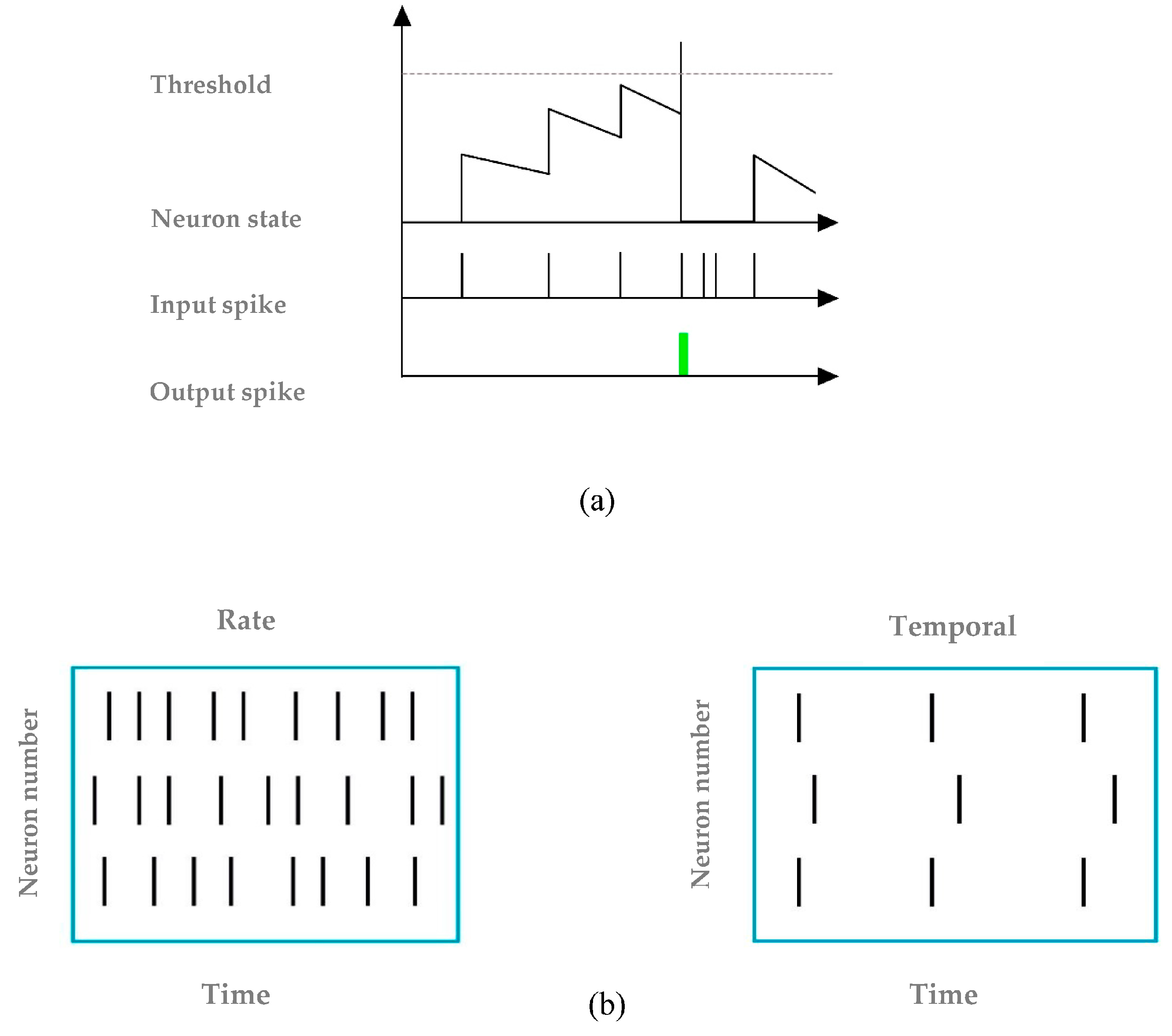
where $S_i^{l-1}$ denotes the spike train and ${\omega }_{ij}^l$ is the input synaptic weight. An output spike occurs when the membrane voltage surpasses the firing threshold ${\mathrm{V}}_j^l\left(\mathrm{t}\right)\ge V_{th}$. Figure 2a depicts an overview of an IF neuron.

3.2. Information Coding

The initial phase of an SNN is the transformation of the original features into spikes to feed the spiking networks. The encoding strategy has a significant effect on network performance. Selecting the best coding strategy depends on the application, hardware limitations, and neuron model [59]. Rate coding is one of the traditional strategies used for encoding information in SNNs, which is based on the spike firing rate. Another popular coding strategy is temporal coding, which encodes information in spike times [60,61]. Figure 2b depicts the schematic of rate and temporal coding. Temporal encoding can be represented mathematically as follows:

$$Y\left(x\right)=\left[\frac{a^{\prime }-a)}{m}\ast x\right]+\left[\frac{\left(a*N\right)-\left(a^{\prime }\ast n\right)}{m}\right]$$

(2)

where $x$ is the original feature value and the maximum and minimum values that $x$ can take are $N$ and $n$. The range between $N$ and $n$ is denoted by $m$, and $Y$ is the spike temporal transformation over the lower and upper temporal interval bounds $\left[a,a^{\prime }\right]$.

In this work, a type of temporal coding called rank-order encoding is used to transform features into spikes [62]. It assumes that strongly activated neurons will tend to fire earlier than weakly activated ones. As compared to rate coding, rank-order coding provides more information with fewer spikes. Another benefit of rank-order coding, compared to rate coding, is that it requires fewer simulation time steps for training. With the use of rank-order coding, the IF neuron can fire at most one spike: the most-activated neurons fire first, while less-activated neurons fire later. Since the network decision is based on the first spike in the output layer, the earlier spikes carry more information.

3.3. Construction of the Error Function

Supervised learning algorithms are based on knowledge of the target values. They try to minimize the error between the desired output (target) and the actual output in order to achieve optimal results. The error function shows the deviation between desired and actual outputs. We determine a temporal fitness function as:

$$e_j=\frac{t_p-t_p^{\prime }}{t_{max}}$$

(3)

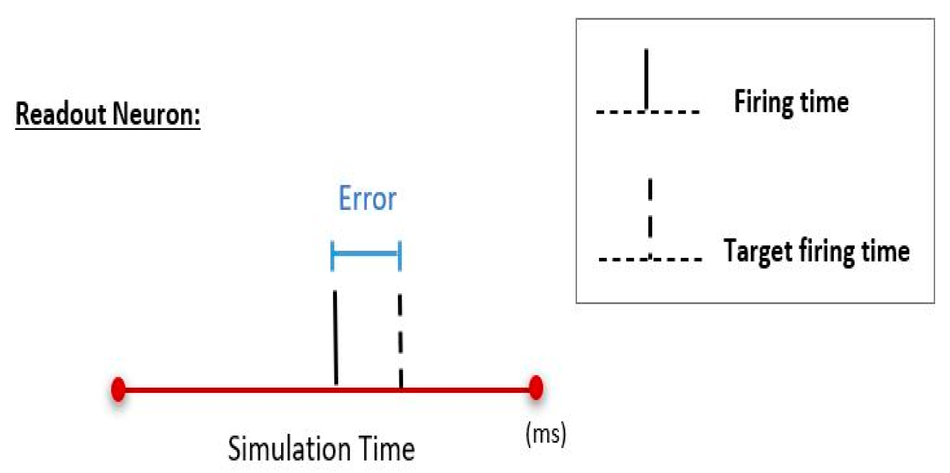
where $t_p$, $t_p^{\prime }$ are the actual firing time and the target firing time of the output neuron, respectively, and $t_{max}$ is the maximum simulation time.

Now, we can define the squared error for C categories (a measure to evaluate the ability of the solution):

$$E_s=\frac{1}{2}{\sum }_{j=1}^C{\left(e_j\right)}^2=\frac{1}{2}{\sum }_{j=1}^C(\frac{t_p-t_p^{\prime }}{t_{max}}{)}^2$$

(4)

The temporal fitness function is considered as the objective function to evaluate each individual. The objective is to minimize the squared error.

3.4. Target Firing Time

As mentioned before, we consider the first readout neuron to fire to classify the input. Instead of defining a predefined target firing time, we use a relative approach to estimate the target firing times [63]. For the input in the $i^{th}$ category, we can determine $\{\begin{array}{c}{t}_{pi}=\tau \\ t_{pj}=t_{max}\end{array}$ for ($j\ne i$), where the desired firing time for the winning neuron is $0<\tau <t_{max}$. The right readout neuron is pushed to fire early in this approach.

The length of the simulation time is determined by the number of classes. To define the duration of the simulation time, we can set time windows (TWs):

$$Simulation Time=\{T{W}_1,T{W}_2, \dots , T{W}_m\}$$

(5)

where m is the number of classes that consist of the classification problem. The duration of each TW is determined by:

$$TW=\frac{Simulation time}{Number of classes}$$

(6)

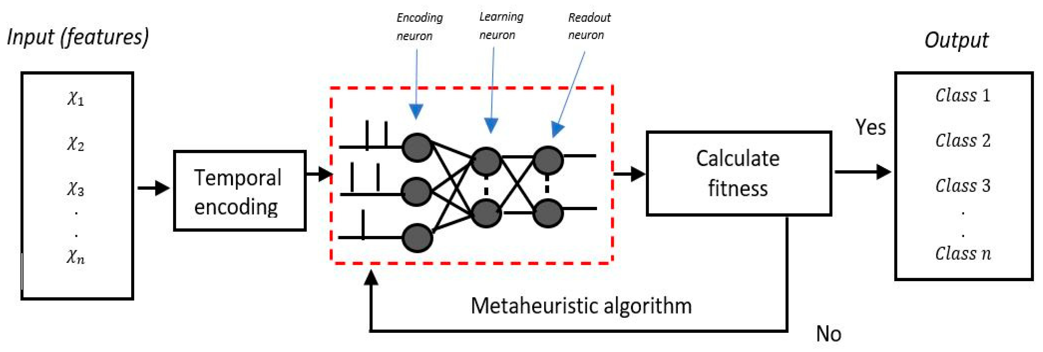
The schematic of the learning process in the SNN based on a metaheuristic algorithm is presented in Figure 3. Figure 4 illustrates the schematic of the readout neuron.

4. Experimental Results and Evaluation

To evaluate the accuracy of the suggested approach, five experiments were implemented. The datasets used were provided by the UCI Machine Learning Repository [64] and were named Pima Indians Diabetes (Diabetes), Iris Plant, Breast Cancer, Wine, and Liver. Each dataset was split into two groups of nearly equal size named the training set and the testing set.

Table 2. Specification of the UCI benchmark datasets.

Name	Source	Size	Features	Classes	Training/Testing
Iris	UCI	150	4	3	75	75
Breast Cancer	UCI	683	9	2	350	333
Diabetes	UCI	786	8	2	384	384
Wine	UCI	178	13	3	105	73
Liver	UCI	345	6	2	200	145

shows the characteristics of the UCI benchmark datasets that were used in this work.

4.1. Iris Plant

The Iris dataset contains 150 samples, divided into three categories (Iris setosa, Iris virginica, and Iris versicolor), each having 50 samples with four attributes. The dataset is divided into 75 samples for training and testing. The dataset was encoded into spikes over the simulation times.

4.2. Breast Cancer

The BCW dataset contains 683 instances, divided into two categories (benign and malignant cell tissues), with 458 benign (65.5%) and 241 (34.5%) samples, respectively. Each class had nine features encoded into spikes over the simulation times. The dataset was split into two parts, training and test datasets, with 342 and 341 samples, respectively.

4.3. Diabetes

The Diabetes dataset contains 768 samples belonging to two classes (with or without signs of diabetes). It includes eight quantitative variables. The dataset was divided into two parts, training and test datasets, which contained equal numbers of samples (384).

4.4. Wine

The Wine dataset contains 178 instances, divided into three categories, with 13 features. The dataset was divided into two parts: training and test datasets, with 105 and 73 samples, respectively. The dataset was encoded into spikes over simulation times.

4.5. Liver

The Liver dataset contains 345 samples belonging to two classes. It includes six quantitative variables. The dataset was divided into two parts, training and test datasets, with 200 and 145 samples, respectively. The dataset was encoded into spikes over simulation times.

All the experiments and performance analyses were programmed in Python. This was run on an Intel corei7 CPU 1.60 GHz processor with 16 GB RAM. In this experiment, the threshold of all neurons in all layers was set to 100. We set the maximum simulation time as $t_{max}$ = 256 and initialized the synaptic weights with random values drawn from uniform distributions in the range [0, 1]. There were also specific parameters associated with each metaheuristic algorithm, as presented in

Table 3. Specific parameters of the metaheuristic algorithms.

Algorithm	Parameters
GA	Epoch = 20, Population size = 100, Crossover rate = 0.6, Mutation rate = 0.05
DE	F = 0.9, CR = 0.8
PSO	$V_{max}$ = 4, $V_{min}$ = −4, $c_1$ and $c_2$ = 2, $X_{max}$ = 10, $X_{min}$ = −10
CS	Pa = 0.25, $X_{max}$ = 10, $X_{min}$ = −10
HS	Par = 0.4, $HMCR$ = 0.9, $BW$ = 0.01
ABC	Population size = 100, MCN = 20, LIM = 100
GE	Population size = 100, Boundaries ∈ [0, 255]

. We tested various values for each parameter and selected the one that led to the highest accuracy. Each algorithm was tested for 20 iterations.

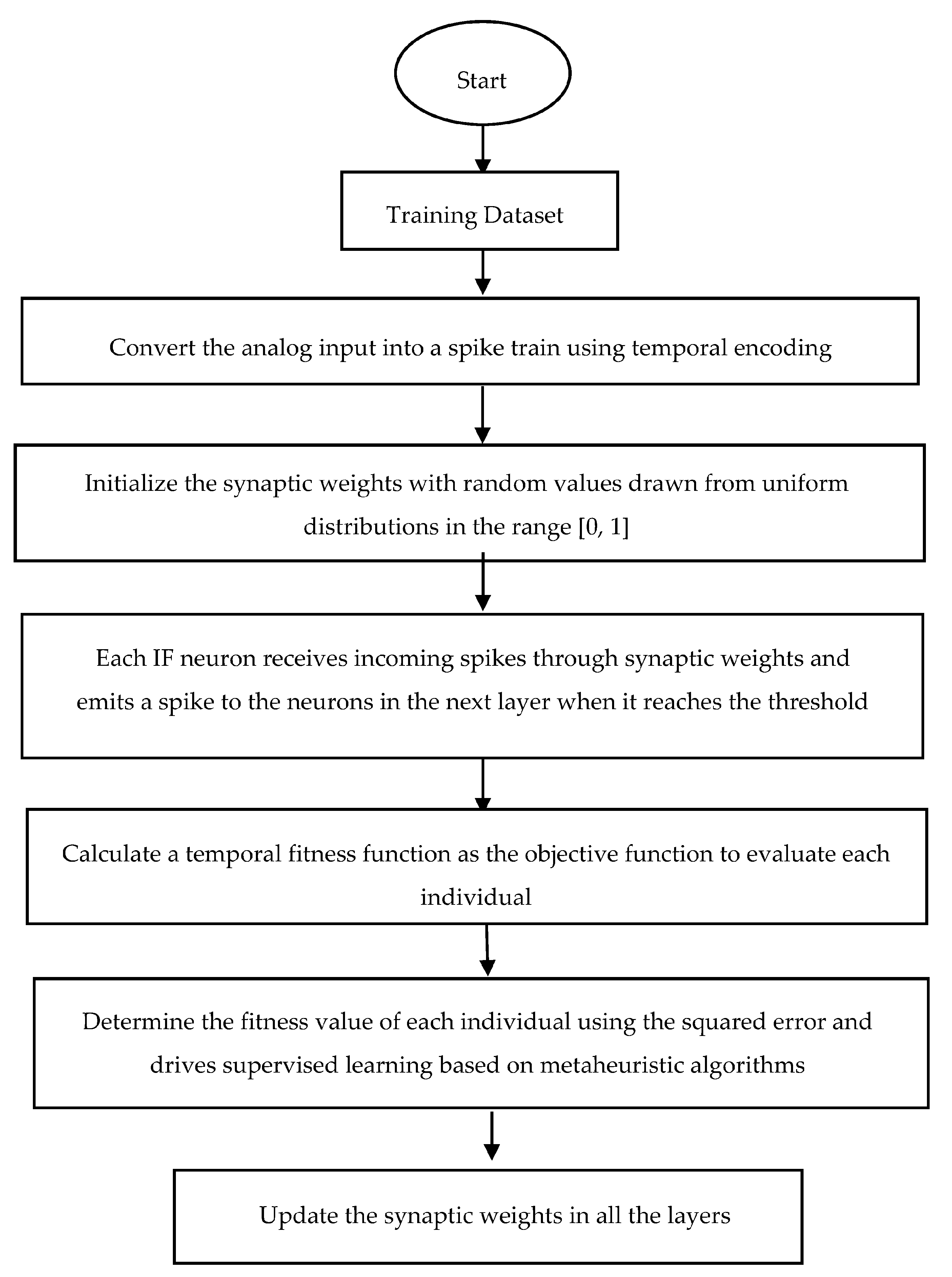
In this work, we present a metaheuristic-based supervised learning method for SNNs, as shown in Figure 5. The following sequential steps describe the learning procedure of the proposed method:

(1)

The first step is to transform the analog input into a spike train. Here, we used temporal coding for the entry layer. These spikes are then fed to the first layer of the network, where the IF neuron receives incoming spikes through synaptic weights and emits a spike to the neurons in the next layer when it reaches the threshold (Equation (1)). We initialized the input-hidden synaptic weights based on random values in the range [0, 1].

(2)

For the classification task with the N class, each output neuron was assigned to a different class. After the forward pass was completed, the output neuron in the readout layer that fired earlier determined the class of the stimulus. Thus, to be able to train the network in the backward pass, we defined a temporal fitness function for the output layer by comparing its actual firing time and the target firing time (Equation (3)).

(3)

During the training phase, we used metaheuristic algorithms to update the synaptic weights. The temporal fitness function was considered as the objective function to evaluate each individual. The next step is to calculate the squared error for N classes using Equation (4). This calculated error determines the fitness value of each individual and drives supervised learning based on metaheuristic algorithms. After completing the forward and backward steps on the current input, the membrane potentials of all the IF neurons are reset to zero, and the network gets ready to process the next input. In order to evaluate the performance of the system, after the training phase, the weights were updated, fixed, and the testing datasets were fed into the network so that the classification accuracy of the testing datasets could be calculated. The first output neuron to fire determines the decision of the network.

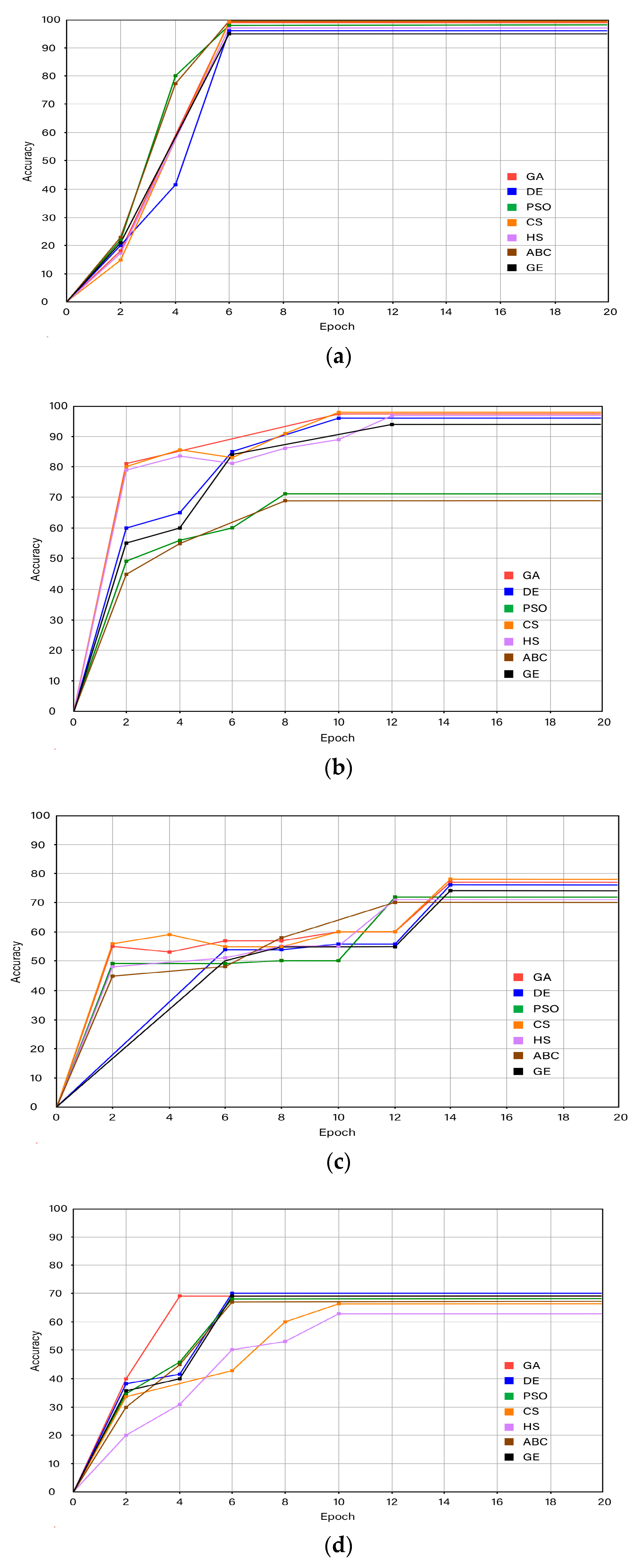
The learning curve of the proposed method is illustrated in Figure 6. It illustrates the changes in the learning accuracy value over 20 iterations. It is clear that, as iterations increase, all algorithms eventually converge. The learning curve results of the algorithms are displayed in various colors. The red line indicates the learning curve of GA, the green line indicates that of PSO, the purple line that of HS, the blue line that of DE, the orange line that of SC, the black line that of GE, and the brown line that of ABC. The learning curves show that CS outperformed these experimental algorithms in five datasets, namely, Iris, Cancer, Wine, Diabetes, and Liver. For example, for the Iris dataset, the accuracy was increased at iteration 2 from 0 to 15. The accuracy was then increased to 99.76 at iteration 6 and remained unchanged until all iterations were completed.

The classification accuracy (CA) obtained with different metaheuristic algorithms was calculated as:

$$CA=\frac{n}{N}$$

(7)

where N and n are the total number of categories and the number of accurate classes, respectively.

5. Discussion

The performance of the metaheuristic-based supervised learning was evaluated on five datasets provided by the UCI Machine Learning Repository: Pima Indians Diabetes (Diabetes), Iris Plant, Breast Cancer, Wine, and Liver. The population size and the number of iterations for all datasets were set to 100 and 20, respectively. We investigated the performance of seven meta-heuristic algorithms named the Cuckoo Search Algorithm, Genetic Algorithm, Differential Evolution, Harmony Search, Particle Swarm Optimization, Grammatical Evolution, and Artificial Bee Colony as training algorithms for SNNs. We employed a relative approach to estimate target firing times instead of defining a predefined target firing time.

According to the learning curve in Figure 6, it can be observed that all algorithms converged to the optimal solution; however, the CS algorithm showed a faster convergence rate, particularly for the four datasets Iris, Cancer, Wine, and Diabetes. After only six iterations, the CS algorithm converged to the optimal solution. For liver classification, the DE algorithm had a faster convergence rate after only six iterations.

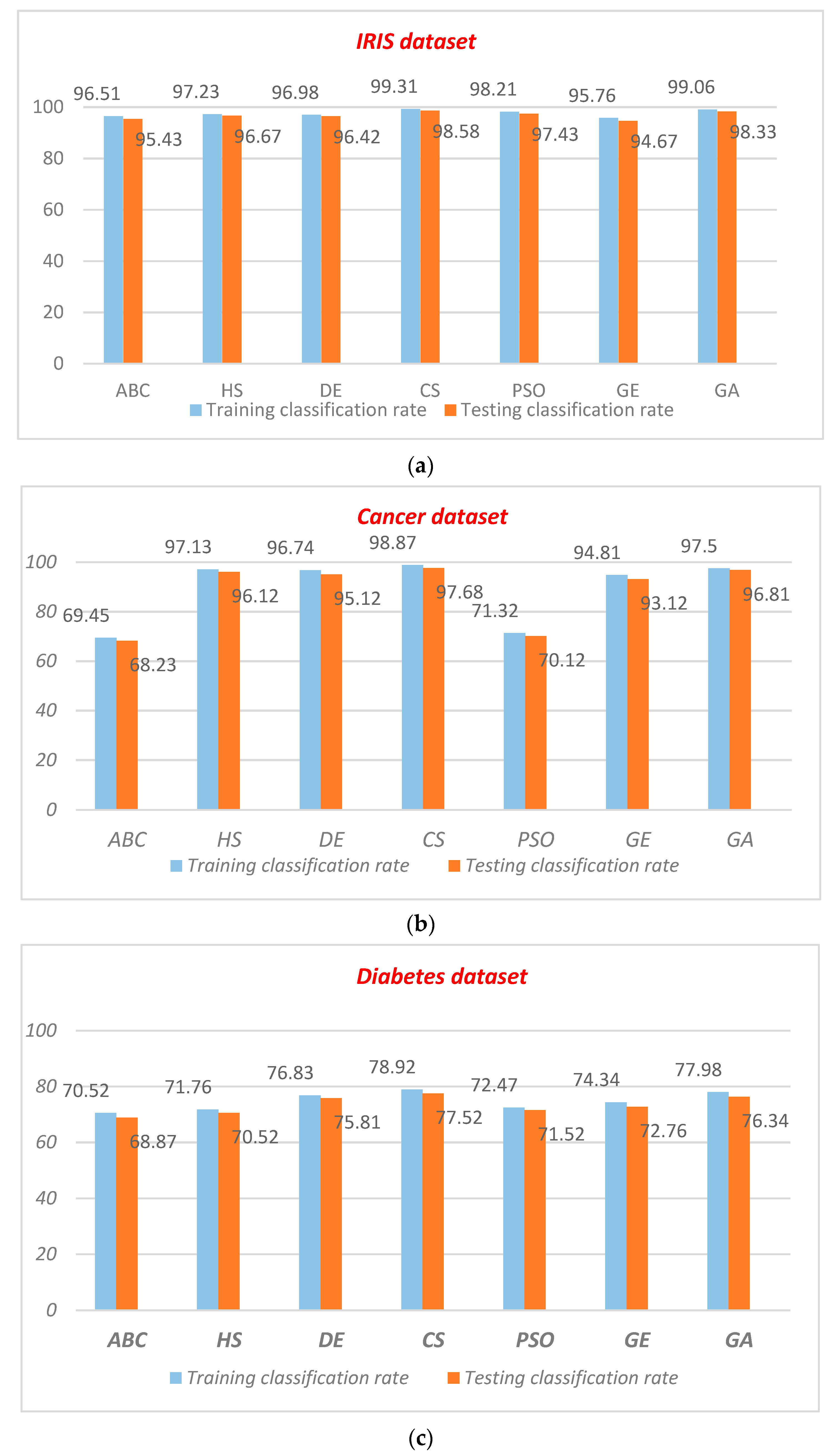
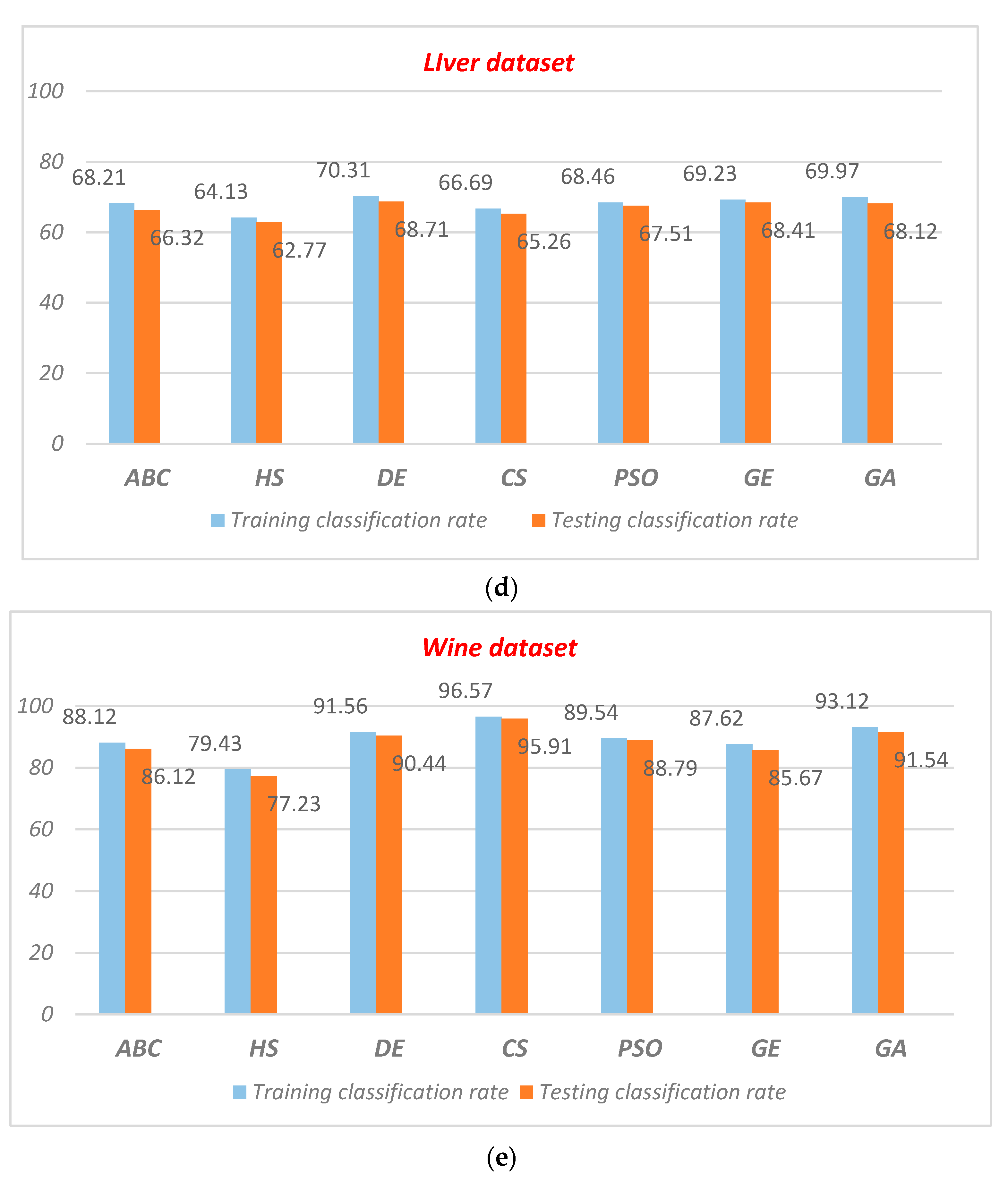
The trained network was then tested on the test dataset. Figure 7 shows the training and testing results of UCI datasets among all metaheuristic designs. Based on the classification accuracy achieved by the seven metaheuristic algorithms, it is evident that all of the algorithms gave comparable performances. For the Iris dataset, the classification accuracy of CS was the highest; the training and testing classification accuracies were 99.31% and 98.58%, respectively. In contrast, GE achieved the lowest classification accuracy; training and testing accuracies were 95.76% and 94.67%, respectively. For the Cancer dataset, the classification accuracy of CS on the training and testing sets was 98.87% and 97.68%, which results were superior to those for the other algorithms. For the Liver dataset, the classification accuracy of GA on the training and testing sets was 69.97% and 68.12%—higher than CS and PSO, but lower than DE. For the Wine and Diabetes datasets, CS achieved much better accuracy than the other algorithms.

Furthermore, in order to validate the efficiency of the proposed algorithm, five experiments were performed, and the quantitative results were compared with other supervised learning algorithms using multilayer feedforward SNNs. In Table 3, the various models for developing supervised SNNs are compared in terms of learning type and approaches, spiking neuron models, encoding methods, and accuracy based on the five datasets: Pima Indians Diabetes (Diabetes), Iris Plant, Breast Cancer Wisconsin, Wine, and Liver. The gradient descent algorithm SpikeProp [65], Enhanced-Mussels Wandering Optimization (E-MWO) [66], SpikeTemp [67], Growing-Pruning (GP) [68], and multi-SNN with Long-Term Memory SRM [69] were chosen for comparison.

Table 4. Summary of the models for developing supervised SNNs—their learning techniques, neuron models, and encoding strategies, along with their accuracy rates on the UCI dataset.

Work	Learning Type	Learning Technique	Spiking Neuron Model	Encoding Information	Dataset	Accuracy
SpikeProp [65]	Supervised	Gradient descent rule	Spike Response Model	Gaussian Receptive Field population encoding	Iris	0.961
					Cancer	0.97
					Diabetes	0.762
					Liver	0.651
					Wine	0.968
E-MWO [66]	Supervised	Enhanced-Mussels Wandering Optimization algorithm	Spike Response Model	Min–max data normalization	Iris	0.913
					Cancer	0.949
					Diabetes	0.706
GPSNN [68]	Supervised	Two-stage learning	Leaky Integrate-and-Fire	Modified population coding	Iris	0.965
					Cancer	0.964
					Diabetes	0.7161
					Liver	0.5979
Multi-SNN [69]	Supervised	Gradient descent rule	Long-term memory Spike Response Model	Population coding	Iris	0.972
					Cancer	0.949
					Diabetes	0.718
					Liver	0.647
SpikeTemp [67]	Supervised	Enhanced rank-order-based learning	Integrate-and-Fire	Gaussian Receptive Field population encoding	Iris	0.95
					Cancer	0.921
					Diabetes	0.703
					Liver	0.522
This work	Supervised	Metaheuristic-based supervised learning	Integrate-and-Fire	Temporal coding	Iris	CS_SNN = 0.9858
					Cancer	CS_SNN = 0.9768
					Diabetes	CS_SNN = 0.7752
					Liver	DE_SNN = 0.6871
					Wine	CS_SNN = 0.9591

shows that the proposed model outperformed the other algorithms in terms of classification accuracy. The suggested approach achieved optimal results on four classification test datasets. As shown by the simulation results in Table 4, for the Iris dataset, the classification accuracy of our proposed model was 98.58%, which was higher than for all the other models. Close to our result, the multi-SNN with Long-Term Memory SRM had an accuracy of 97.2%. For the Breast Cancer dataset, the classification accuracy of the proposed algorithm was 97.68%. The accuracy of SpikeProp was 97%, which was around 0.68% lower than our best model. SpikeTemp, a rank-order based learning method for SNNs, however, obtained the lowest accuracy of 92.1%. For the Diabetes dataset, our best model scored 77.52%, which was higher than the scores for all the other models. For the Wine dataset, the classification accuracy of our proposed model was 95.91%, but 0.9% lower than SpikeProp. For the Liver dataset, our best model achieved an accuracy of 68.71%. The accuracies of SpikeProp and multi-SNN were 65.1% and 64.7%, respectively. SpikeTemp and Growing-Pruning (GP) obtained the lowest accuracies of 55.2% and 59.79%, respectively.

We also compared the efficiency of the proposed algorithm with some existing non-spiking models for solving classification problems with medical data. Darabi et al. (2021) presents a thermogram-based Computer-Aided Detection (CAD) system for breast cancer detection [70]. In this CAD system, the Random Subset Feature Selection (RSFS) algorithm and a hybrid of the minimum Redundancy Maximum Relevance (mRMR) algorithm and GA with the RSFS algorithm are utilized for feature selection. The experimental results demonstrate that using the RSFS algorithm for feature selection and kNN and SVM algorithms as classifiers have 85.36% and 75% accuracy, respectively. Additionally, using hybrid GA and RSFS algorithms for feature selection and kNN and SVM algorithms for classifiers yielded 83.87% and 69.56% accuracy, respectively.

In another study, Zarei et al. (2021) proposed a novel segmentation method for breast cancer detection using infrared thermal images [71]. The evaluation results showed that the average Dice similarity coefficient, Jaccard index, and Hausdorff distance in the FCM segmentation algorithm were 89.44%, 80.90% and 5.00, respectively. These values were 89.30%, 80.66%, and 5.15 for the MS segmentation algorithm, and 91.81%, 84.86%, and 4.87 for the MGMS segmentation algorithm. Salman et al. (2018) proposed a hybrid classification optimization method for improving ANN classification accuracy [72]. Three optimization approaches named GA, PSO, and Fireworks Algorithm (FWA) were used in this work. They achieved an accuracy of 98.42% on the breast cancer datasets. In general, our proposed approach demonstrated competitive accuracy on the UCI datasets.

6. Conclusions

In this paper, we have demonstrated how different metaheuristic algorithms called Cuckoo Search, Genetic Algorithm, Harmony Search, Differential Evolution, Particle Swarm Optimization, Artificial Bee Colony, and Grammatical Evolution, can be applied to train a spiking neural network. This approach effectively avoids some problems, such as getting stuck in local minima and over-fitting. In the input layer, a temporal coding scheme is used to transform input data into spikes. Leaky Integrate-and-Fire neurons are employed to simulate the hidden and output layer neurons. The training process for the neurons was carried out using metaheuristic algorithms. We employed dynamic approaches to determine the target firing times for each input. The performance of our approach was evaluated on five UCI Machine Learning Repository datasets. The CS successfully obtained accuracies of 0.9858, 0.9768, 0.9591, and 0.7752 for the Iris, Cancer, Wine, and Diabetes datasets, respectively. DE showed the best performance for the Liver dataset (0.6871). The classification accuracy of the proposed learning model was compared to some existing non-metaheuristic training algorithms. Several issues need to be tackled before an SNN can be used for various tasks, including the design of a learning algorithm. Future work will include conducting experiments on more complex pattern-recognition problems, such as face and voice recognition, with more complex datasets and investigation of the impact of different encoding schemes on classification accuracy. Furthermore, designing a multi-objective fitness function using algorithms, such as Bayesian optimization, is needed to produce the most accurate and smallest SNNs.

References

1. Zhang, C.; Lu, Y. Study on artificial intelligence: The state of the art and prospects. J. Ind. Inf. Integr. 2021, 23, 100224. [Google Scholar] [CrossRef]
2. Apostolidis, E.; Adamantidou, E.; Metsai, A.I.; Mezaris, V.; Patras, I. Video summarization using deep neural networks: A survey. Proc. IEEE 2021, 109, 1838–1863. [Google Scholar] [CrossRef]
3. Syed, F.; Gupta, S.K.; Hamood Alsamhi, S.; Rashid, M.; Liu, X. A survey on recent optimal techniques for securing unmanned aerial vehicles applications. Trans. Emerg. Telecommun. Technol. 2021, 32, e4133. [Google Scholar]
4. Khurana, D.; Koli, A.; Khatter, K.; Singh, S. Natural language processing: State of the art, current trends and challenges. Multimed. Tools Appl. 2023, 82, 3713–3744. [Google Scholar] [CrossRef] [PubMed]
5. Giger, M.L. Machine learning in medical imaging. J. Am. Coll. Radiol. 2018, 15, 512–520. [Google Scholar] [CrossRef]
6. Skinner, G.; Walmsley, T. Artificial intelligence and deep learning in video games a brief review. In Proceedings of the 4th International Conference on Computer and Communication Systems (ICCCS), Singapore, 23–25 February 2019; pp. 404–408. [Google Scholar]
7. Wu, H.; Liu, Y.; Wang, J. Review of text classification methods on deep learning. Comput. Mater. Contin. 2020, 63, 1309. [Google Scholar] [CrossRef]
8. Maass, W. Networks of spiking neurons: The third generation of neural network models. Neural Netw. 1997, 10, 1659–1671. [Google Scholar] [CrossRef]
9. Jang, H.; Simeone, O.; Gardner, B.; Gruning, A. An introduction to probabilistic spiking neural networks: Probabilistic models, learning rules, and applications. IEEE Signal Process. Mag. 2019, 36, 64–77. [Google Scholar] [CrossRef] [Green Version]
10. Wang, S.; Cheng, T.H.; Lim, M.H. A hierarchical taxonomic survey of spiking neural networks. Memetic Comput. 2022, 14, 335–354. [Google Scholar] [CrossRef]
11. Yamazaki, K.; Vo-Ho, V.-K.; Bulsara, D.; Le, N. Spiking Neural Networks and Their Applications: A Review. Brain Sci. 2022, 12, 863. [Google Scholar] [CrossRef]
12. Belatreche, A. Biologically Inspired Neural Networks; OmniScriptum Publishing: Riga, Latvia, 2010. [Google Scholar]
13. Deng, L.; Tang, H.; Roy, K. Understanding and bridging the gap between neuromorphic computing and machine learning. Front. Comput. Neurosci. 2021, 15, 665662. [Google Scholar] [CrossRef]
14. Roy, K.; Jaiswal, A.; Panda, P. Towards spike-based machine intelligence with neuromorphic computing. Nature 2019, 575, 607. [Google Scholar] [CrossRef]
15. Merolla, P.A.; Arthur, J.V.; Alvarez-Icaza, R.; Cassidy, A.S.; Sawada, J.; Akopyan, F.; Modha, D.S. A million spiking-neuron integrated circuit with a scalable communication network and interface. Science 2014, 345, 668–673. [Google Scholar] [CrossRef]
16. Davies, M.; Srinivasa, N.; Lin, T.H.; Chinya, G.; Cao, Y.; Choday, S.H.; Liao, Y. Loihi: A neuromorphic manycore processor with on-chip learning. IEEE Micro 2018, 38, 82–99. [Google Scholar] [CrossRef]
17. Furber, S. Large-scale neuromorphic computing systems. J. Neural Eng. 2016, 13, 051001. [Google Scholar] [CrossRef]
18. Liao, J.; Widmer, L.; Wang, X.; Di Mauro, A.; Nason-Tomaszewski, S.R.; Chestek, C.A.; Jang, T. An energy-efficient spiking neural network for finger velocity decoding for implantable brain-machine interface. In Proceedings of the 4th International Conference on Artificial Intelligence Circuits and Systems (AICAS), Incheon, Republic of Korea, 13–15 June 2022; pp. 134–137. [Google Scholar]
19. Tang, G.; Michmizos, K.P. Gridbot: An autonomous robot controlled by a spiking neural network mimicking the brain’s navigational system. In Proceedings of the International Conference on Neuromorphic Systems, Knoxville, TN, USA, 23–26 July 2018; pp. 1–8. [Google Scholar]
20. Osswald, M.; Ieng, S.H.; Benosman, R.; Indiveri, G. A spiking neural network model of 3D perception for event-based neuromorphic stereo vision systems. Sci. Rep. 2017, 7, 40703. [Google Scholar] [CrossRef] [Green Version]
21. Tavanaei, A.; Ghodrati, M.; Kheradpisheh, S.R.; Masquelier, T.; Maida, A. Deep learning in spiking neural networks. Neural Netw. 2019, 111, 47–63. [Google Scholar] [CrossRef] [Green Version]
22. Dora, S.; Kasabov, N. Spiking Neural Networks for Computational Intelligence: An Overview. Big Data Cogn. Comput. 2021, 5, 67. [Google Scholar] [CrossRef]
23. Cao, Y.; Chen, Y.; Khosla, D. Spiking deep convolutional neural networks for energy-efficient object recognition. Int. J. Comput. Vis. 2015, 113, 54–66. [Google Scholar] [CrossRef]
24. Hu, Y.; Tang, H.; Pan, G. Spiking deep residual networks. IEEE Trans. Neural Netw. Learn. Syst. 2021, 1–6. [Google Scholar] [CrossRef]
25. Diehl, P.U.; Neil, D.; Binas, J.; Cook, M.; Liu, S.C.; Pfeiffer, M. Fast-classifying, high-accuracy spiking deep networks through weight and threshold balancing. In Proceedings of the International Joint Conference on Neural Networks (IJCNN), Killarney, Ireland, 12–16 July 2015; pp. 1–8. [Google Scholar]
26. Sengupta, A.; Ye, Y.; Wang, R.; Liu, C.; Roy, K. Going deeper in spiking neural networks: VGG and residual architectures. Front. Neurosci. 2019, 13, 95. [Google Scholar] [CrossRef] [PubMed] [Green Version]
27. Rueckauer, B.; Lungu, I.A.; Hu, Y.; Pfeiffer, M.; Liu, S.C. Conversion of continuous-valued deep networks to efficient event-driven networks for image classification. Front. Neurosci. 2017, 11, 682. [Google Scholar] [CrossRef] [PubMed] [Green Version]
28. Han, B.; Srinivasan, G.; Roy, K. Rmp-snn: Residual membrane potential neuron for enabling deeper high-accuracy and low-latency spiking neural network. In Proceedings of the IEEE/CVF Conference on Computer Vision and Pattern Recognition, Seattle, WA, USA, 13–19 June 2020; pp. 13558–13567. [Google Scholar]
29. Caporale, N.; Dan, Y. Spike timing—Dependent plasticity: A Hebbian learning rule. Annu. Rev. Neurosci. 2008, 31, 25–46. [Google Scholar] [CrossRef] [PubMed] [Green Version]
30. Mozafari, M.; Ganjtabesh, M.; Nowzari-Dalini, A.; Thorpe, S.J.; Masquelier, T. Bio-inspired digit recognition using reward-modulated spike-timing-dependent plasticity in deep convolutional networks. Pattern Recognit. 2019, 94, 87–95. [Google Scholar] [CrossRef] [Green Version]
31. Kheradpisheh, S.; Ganjtabesh, M.; Thorpe, S. STDP-based spiking deep convolutional neural networks for object recognition. Neural Netw. 2018, 99, 56–67. [Google Scholar] [CrossRef] [Green Version]
32. Diehl, P.U.; Cook, M. Unsupervised learning of digit recognition using spike-timing-dependent plasticity. Front. Comput. Neurosci. 2015, 9, 99. [Google Scholar] [CrossRef] [Green Version]
33. Masquelier, T.; Thorpe, S.J. Unsupervised learning of visual features through spike timing dependent plasticity. PLoS Comput. Biol. 2007, 3, e31. [Google Scholar] [CrossRef] [Green Version]
34. Taherkhani, A.; Belatreche, A.; Li, Y.; Cosma, G.; Maguire, L.; McGinnity, T. A review of learning in biologically plausible spiking neural networks. Neural Netw. 2020, 122, 253–272. [Google Scholar] [CrossRef]
35. Bohte, S.M.; Kok, J.N.; La Poutre, H. Error-backpropagation in temporally encoded networks of spiking neurons. Neurocomputing 2002, 48, 17–37. [Google Scholar] [CrossRef] [Green Version]
36. Ponulak, F.; Kasiński, A. Supervised learning in spiking neural networks with ReSuMe: Sequence learning, classification, and spike shifting. Neural Comput. 2010, 22, 467–510. [Google Scholar] [CrossRef]
37. Gütig, R.; Sompolinsky, H. The tempotron: A neuron that learns spike timing–based decisions. Nat. Neurosci. 2006, 9, 420–428. [Google Scholar] [CrossRef]
38. Mohemmed, A.; Schliebs, S.; Matsuda, S.; Kasabov, N. Span: Spike pattern association neuron for learning spatio-temporal spike patterns. Int. J. Neural Syst. 2012, 22, 1250012. [Google Scholar] [CrossRef]
39. Ojha, V.K.; Abraham, A.; Snášel, V. Metaheuristic design of feedforward neural networks: A review of two decades of research. Eng. Appl. Artif. Intell. 2017, 60, 97–116. [Google Scholar] [CrossRef] [Green Version]
40. Kaveh, M.; Mesgari, M.S. Application of meta-heuristic algorithms for training neural networks and deep learning architectures: A comprehensive review. Neural Process. Lett. 2022, 1–104. [Google Scholar] [CrossRef]
41. Pavlidis, N.G.; Tasoulis, O.K.; Plagianakos, V.P.; Nikiforidis, G.; Vrahatis, M.N. Spiking neural network training using evolutionary algorithms. In Proceedings of the International Joint Conference on Neural Networks, Montreal, QC, Canada, 31 July–4 August 2005; Volume 4, pp. 2190–2194. [Google Scholar]
42. Vázquez, R.A.; Garro, B.A. Training spiking neurons by means of particle swarm optimization. In Proceedings of the International Conference in Swarm Intelligence, Chongqing, China, 12–15 June 2011; pp. 242–249. [Google Scholar]
43. Vazquez, R.A.; Garro, B.A. Training spiking neural models using artificial bee colony. Comput. Intell. Neurosci. 2015, 2015, 18. [Google Scholar] [CrossRef] [Green Version]
44. Rere, L.M.; Fanany, M.I.; Arymurthy, A.M. Metaheuristic algorithms for convolution neural network. Comput. Intell. Neurosci. 2016, 2016, 13. [Google Scholar] [CrossRef] [Green Version]
45. Ghasemi-Marzbali, A. A novel nature-inspired meta-heuristic algorithm for optimization: Bear smell search algorithm. Soft Comput. 2020, 24, 13003–13035. [Google Scholar] [CrossRef]
46. Holland, J.H. Adaptation in Natural and Artificial Systems: An Introductory Analysis with Applications to Biology, Control, and Artificial Intelligence; MIT Press: Cambridge, MA, USA, 1992. [Google Scholar]
47. Slowik, A.; Kwasnicka, H. Evolutionary algorithms and their applications to engineering problems. Neural Comput. Appl. 2020, 32, 12363–12379. [Google Scholar] [CrossRef] [Green Version]
48. Pant, M.; Zaheer, H.; Garcia-Hernandez, L.; Abraham, A. Differential Evolution: A review of more than two decades of research. Eng. Appl. Artif. Intell. 2020, 90, 103479. [Google Scholar]
49. Mareli, M.; Twala, B. An adaptive Cuckoo search algorithm for optimisation. Appl. Comput. Inform. 2018, 14, 107–115. [Google Scholar] [CrossRef]
50. Shami, T.M.; El-Saleh, A.A.; Alswaitti, M.; Al-Tashi, Q.; Summakieh, M.A.; Mirjalili, S. Particle swarm optimization: A comprehensive survey. IEEE Access 2022, 10, 10031–10061. [Google Scholar] [CrossRef]
51. Ala’a, A.; Alsewari, A.A.; Alamri, H.S.; Zamli, K.Z. Comprehensive review of the development of the harmony search algorithm and its applications. IEEE Access 2019, 7, 14233–14245. [Google Scholar]
52. Karaboga, D.; Basturk, B. A powerful and efficient algorithm for numerical function optimization: Artificial bee colony (ABC) algorithm. J. Glob. Optim. 2007, 39, 459–471. [Google Scholar] [CrossRef]
53. O’Neill, M.; Ryan, C. Grammatical evolution. IEEE Trans. Evol. Comput. 2001, 5, 349–358. [Google Scholar] [CrossRef] [Green Version]
54. Gerstner, W.; Kistler, W.M.; Naud, R.; Paninski, L. Neuronal Dynamics: From Single Neurons to Networks and Models of Cognition; Cambridge University Press: Cambridge, MA, USA, 2014. [Google Scholar]
55. Izhikevich, E.M. Simple model of spiking neurons. IEEE Trans. Neural Netw. 2003, 14, 1569–1572. [Google Scholar] [CrossRef] [Green Version]
56. Lecar, H. Morris-lecar model. Scholarpedia 2007, 2, 1333. [Google Scholar] [CrossRef]
57. Izhikevich, E.M.; FitzHugh, R. Fitzhugh-nagumo model. Scholarpedia 2006, 1, 1349. [Google Scholar] [CrossRef]
58. Hodgkin, A.L.; Huxley, A.F. A quantitative description of membrane current and its application to conduction and excitation in nerve. J. Physiol. 1952, 117, 500. [Google Scholar] [CrossRef]
59. Javanshir, A.; Nguyen, T.T.; Mahmud, M.P.; Kouzani, A.Z. Advancements in Algorithms and Neuromorphic Hardware for Spiking Neural Networks. Neural Comput. 2022, 34, 1289–1328. [Google Scholar] [CrossRef]
60. Kiselev, M. Rate coding vs. temporal coding-is optimum between? In Proceedings of the International Joint Conference on Neural Networks (IJCNN), Vancouver, BC, Canada, 24–29 July 2016; pp. 1355–1359. [Google Scholar]
61. Brette, R. Philosophy of the spike: Rate-based vs. spike-based theories of the brain. Front. Syst. Neurosci. 2015, 9, 151. [Google Scholar] [CrossRef] [Green Version]
62. Tang, H.; Cho, D.; Lew, D.; Kim, T.; Park, J. Rank order coding based spiking convolutional neural network architecture with energy-efficient membrane voltage updates. Neurocomputing 2020, 407, 300–312. [Google Scholar] [CrossRef]
63. Kheradpisheh, S.R.; Masquelier, T. Temporal backpropagation for spiking neural networks with one spike per neuron. Int. J. Neural Syst. 2020, 30, 2050027. [Google Scholar] [CrossRef]
64. Dua, D.; Graff, C. UCI Machine Learning Repository, Irvine, CA. University of California. 2019. Available online: https://archive.ics.uci.edu/ml (accessed on 1 October 2022).
65. Bohte, S.M.; Kok, J.N.; La Poutré, J.A. SpikeProp: Backpropagation for networks of spiking neurons. ESANN 2000, 48, 419–424. [Google Scholar]
66. Abusnaina, A.A.; Abdullah, R.; Kattan, A. Supervised training of spiking neural network by adapting the E-MWO algorithm for pattern classification. Neural Process. Lett. 2019, 49, 661–682. [Google Scholar] [CrossRef]
67. Wang, J.; Belatreche, A.; Maguire, L.P.; McGinnity, T.M. Spiketemp: An enhanced rank-order-based learning approach for spiking neural networks with adaptive structure. IEEE Trans. Neural Netw. Learn. Syst. 2015, 28, 30–43. [Google Scholar] [CrossRef] [Green Version]
68. Dora, S.; Sundaram, S.; Sundararajan, N. A two-stage learning algorithm for a growing-pruning spiking neural network for pattern classification problems. In Proceedings of the International Joint Conference on Neural Networks (IJCNN), Killarney, Ireland, 12–15 July 2015; pp. 1–7. [Google Scholar]
69. Lin, X.; Zhang, M.; Wang, X. Supervised learning algorithm for multilayer spiking neural networks with long-term memory spike response model. Comput. Intell. Neurosci. 2021, 2021, 8592824. [Google Scholar] [CrossRef]
70. Darabi, N.; Rezai, A.; Hamidpour, S.S.F. Breast cancer detection using RSFS-based feature selection algorithms in thermal images. Biomed. Eng. Appl. Basis Commun. 2021, 33, 2150020. [Google Scholar] [CrossRef]
71. Zarei, M.; Rezai, A.; Falahieh Hamidpour, S.S. Breast cancer segmentation based on modified Gaussian mean shift algorithm for infrared thermal images. Comput. Methods Biomech. Biomed. Eng. Imaging Vis. 2021, 9, 574–580. [Google Scholar] [CrossRef]
72. Salman, I.; Ucan, O.N.; Bayat, O.; Shaker, K. Impact of metaheuristic iteration on artificial neural network structure in medical data. Processes 2018, 6, 57. [Google Scholar] [CrossRef] [Green Version]
Figure 1. Three generations of ANNs: multilayer perceptron, McCulloch–Pitts neuron, and SNNs.
Applsci 13 04809 g001
Figure 2. (a) An overview of an IF neuron. Whenever the membrane voltage exceeds the firing threshold, an output spike occurs. (b) Schematic representation of rate and temporal coding. In a temporal-based encoding, information is encoded through specific spike times, whereas the rate encoding is based on a spiking feature during a time interval.
Applsci 13 04809 g002
Figure 3. Generic schemes explaining the learning process of SNNs with metaheuristic algorithms.
Applsci 13 04809 g003
Figure 4. Generic scheme of readout neuron.
Applsci 13 04809 g004
Figure 5. The process of training an SNN using metaheuristic algorithms.
Applsci 13 04809 g005
Figure 6. The training curve of the proposed algorithm on seven datasets, including (a) Iris, (b) Cancer, (c) Diabetes, (d) Liver, and (e) Wine. The red line indicates the learning curve of GA, the blue line that of DE, the green line that of PSO, the orange line that of SC, the purple line that of Harmony Search, the black line that of GE, and the brown line that of ABC.
Applsci 13 04809 g006aApplsci 13 04809 g006b
Figure 7. Classification rate of the training and testing results for seven datasets, including (a) Iris, (b) Cancer, (c) Diabetes, (d) Liver, and (e) Wine.
Applsci 13 04809 g007aApplsci 13 04809 g007b