Lightweight Model for Botnet Attack Detection in Software Defined Network-Orchestrated IoT

Abstract

The Internet of things (IoT) is being used in a variety of industries, including agriculture, the military, smart cities and smart grids, and personalized health care. It is also being used to control critical infrastructure. Nevertheless, because the IoT lacks security procedures and lack the processing power to execute computationally costly antimalware apps, they are susceptible to malware attacks. In addition, the conventional method by which malware-detection mechanisms identify a threat is through known malware fingerprints stored in their database. However, with the ever-evolving and drastic increase in malware threats in the IoT, it is not enough to have traditional antimalware software in place, which solely defends against known threats. Consequently, in this paper, a lightweight deep learning model for an SDN-enabled IoT framework that leverages the underlying IoT resource-constrained devices by provisioning computing resources to deploy instant protection against botnet malware attacks is proposed. The proposed model can achieve 99% precision, recall, and F1 score and 99.4% accuracy. The execution time of the model is 0.108 milliseconds with 118 KB size and 19,414 parameters. The proposed model can achieve performance with high accuracy while utilizing fewer computational resources and addressing resource-limitation issues.

1. Introduction

In the realm of computing, digitization and intervention of AI in different sectors has offered many benefits [1,2,3,4,5,6]. As a result, according to Li and Al Rushdan [7,8], countries’ reliance on digitalization, software-defined networks (SDNs), and the IoT have intensified [9]. The main issue we are dealing with in the age of digitization is cybersecurity. Many sectors of the digital economy can be affected by cyberattacks, which can occasionally result in irreparable harm. They may be responsible for things like electrical blackouts, attacks on financial institutions involving extortion, theft, and fraud, malfunctions of military hardware, and leaks of classified information. These might also result in the theft of valuable personal data that includes sensitive medical information. They may also bring down the systems, which might cause serious negative impacts. According to the Outpost24study, more than 3800 large enterprises faced data breaches in 2019 that resulted in significant impact, as stated in [10]. Despite all of these attacks, there has not been a great deal of awareness about system security, and there have not been many high-quality research findings leading to solutions that can effectively stop malware attacks, according to Pandey et al. [11].

The Internet of things (IoT) is a network of physical objects or devices with integrated electronics, software, and network connectivity that enables these things to gather, occasionally process, and exchange data, according to Suresh [12,13]. The administration of vital infrastructure, agriculture, the military, smart grids and cities, and personal healthcare are just a few of the many applications and services for which the IoT can be used [13]. However, the IoT is vulnerable to malware attacks because it lacks security mechanisms due to limited computational resources to run antimalware applications, low storage capacity, and the fact that it is always connected to the Internet [14]. The IoT is impacted by botnet malware assaults, including Mirai and Prowli attacks. As an alternative, some botnets have been developed to launch a variety of cyberattacks, including identity/data theft (data exfiltration), in which infected machines are used to create and send phony emails, email spam, log keys, and propagate malware.

IoT orchestration with SDN leverages the underlying IoT resource-constrained devices through the provision of computing resources to deploy instant protection for IoT gadgets [15]. Software-defined networking [16] (SDN) is anticipated to be a crucial enabler for next-generation networks, the so-called 5G, which will need to combine both IoT applications and conventional human-based services. In this context, SDN enables a global orchestration of IoT to (a) transport the huge amount of data generated at the terminals, sensors, machines, nodes, etc., to any distributed computing node, edge, or core data center, (b) allocate computing, storage, and network resources, and (c) process the collected data (big data) and make the proper decisions (cognition).

The conventional way by which malware-detection mechanisms identify a threat is through known malware fingerprints stored in their database. For instance, an antiviral engine checks the presence of the malware fingerprint in a file against known malware fingerprints stored in the antivirus database. However, with the ever-evolving and drastic increase in malware threats, it is not enough to have traditional antimalware software in place, which solely defends against known threats. Active protection must be integrated into IoT systems to effectively defend against evolving strains of malware, also known as zero-day threats. Accordingly, nowadays, frameworks that integrate machine learning have been proposed [17,18,19,20]. Sarker et al. [17], in their survey paper, indicated that cybersecurity has massively shifted the technology and its operation. They also claimed that machine learning is paving the way toward a better solution.

The SDN has brought a new approach to the domain of communication networks. It allows network engineers and administrators to install, control, manage, and modify networks. In the SDN network, the gateway is directly connected to the internal network, where all security mechanisms are either installed in the application layer (controlled by the controller for traffic forwarding to the appropriate security device) or installed in the controller layer. Another main difference from a traditional network is that the controller controls every node in the network and can block the nodes’ traffic or forward it to a specific path.

According to Li et al. [21], IoT orchestration with SDN can lessen the security susceptibility of IoT devices. These SDN-enabled frameworks can enhance the potential of the underlying highly dynamic and heterogeneous environment of the IoT network. Deploying the malware-detection module on the control plane of the SDN has several benefits. First, the control plane represents the core centralized intelligence of the SDN and maintains the global view of the entire underlying network. Moreover, all the forwarding decisions are made in the control plane. Secondly, the resource-constrained IoT devices can simply be leveraged from the additional computational task. Furthermore, it allows the use of the antimalware system in a highly manageable and scalable way. Finally, it can be customized and extended to any commercial SDN controller [15].

Machine learning approaches, as opposed to the traditional rule-based programming approach, learn from the dataset gathered from prior experiences to tackle complicated issues. This procedure is completed by using machine learning techniques, including supervised, unsupervised, and reinforcement learning. For instance, Shahzana Liaqat et al. [15] proposed a hybrid deep learning-driven SDN-enabled Internet of medical things (IoMT) malware-detection module to be deployed on the control plane of the SDN.

In this article,

• we discuss an IoT and SDN network orchestration for better security and the vulnerability holes even with the SDN networks,
• we perform a systematic review of the related work to identify the gaps in the previous work done on the same public datasets that we used to propose a new approach that performs better depending on different criteria,
• we reimplement already existing traditional machine learning algorithms and pretrained deep learning models to observe their performance in terms of model evaluation parameters, memory requirement, and computational time requirements, and
• we propose a lightweight deep learning approach that has higher performance in terms of accuracy, precision, recall, F1 score, less computational time, and fewer memory requirements

.

The paper is structured as follows. The related works and previous studies on this topic are presented in Section 2. In Section 3, the dataset, employed approach, and evaluation metrics are covered. In Section 5, the experimental results and comparison to the existing approach are discussed.

2. Related Works

Cybersecurity applications vary in context. Network security, application security, information security, and operational security are the four areas of cybersecurity application. The security and privacy of the relevant data are handled by the information security and the processes of handling and protecting data assets are the responsibility of operational security [22].

There are several types of cybersecurity incidents, and malware represents one of the many types of cybersecurity incidents that are intentionally designed to cause damage to a computer network, server, IoT network, or SDN-IoT orchestrated network [23,24,25]. As a result of cybersecurity challenges, both industry and academia have focused on the development and deployment of machine learning-based malware detection frameworks [18,19].

In the past few years, several traditional machine learning algorithm-based approaches have been proposed and deployed as intrusion-detection mechanisms. Many scholars have employed and assessed a random forest (RF), an ensemble-type classical machine learning technique, to defend SDN-managed IoT networks from botnet attacks like distributed denial of service (DDoS), and denial of service (DoS) [26,27,28]. The detection and mitigation of DoS and DDoS attacks using automated feature extraction from network flow traffic were suggested by Sarica et al. [26]. The RF classifier was trained by using a dataset consisting of six classes created by IoT devices: benign (normal traffic), DDoS, port scanning, fuzzing, DoS, and DDoS was deployed at the SDN application layer. The RF-based model performed very well at distinguishing between regular traffic and botnet attacks like DoS and DDoS. The model’s normal traffic recognition performance was 99.67%, 96.75%, 92.92%, and 94.80%, respectively, in terms of accuracy, precision, recall, and F1 score. Similarly, the model’s precision, recall, and F1 score in detecting the DoS attack were 97.77%, 99.12%, and 98.44%, respectively. The model also performed well in detecting the DDoS attack type, with an F1 score of 97.93%, a precision of 97.29%, and a recall of 98.58%.

The extreme gradient boosting (XGBoost) machine learning algorithm was another approach applied in botnet infection in SDN-enabled IoT networks [29] that uses CICDoS2019, NSL-KDD, and CAIDA-DDoS datasets to train and test the model. The XGBoost was then trained for binary classes to categorize network traffic as a DDoS assault or regular [29] activity by using a variety of attributes that offers the best descriptive information. The accuracy, precision, recall, and F1 score are the model-evaluation parameters used in the authors’ work. As a consequence, the model’s accuracy, precision, recall, and F1 score in the real-time IoT managed on SDN reached more than 99.98%. Similar to this, Swami et al. [30] have suggested AdaBoost-based DDoS attack detection in an SDN-based network, and the model’s accuracy, precision, recall, and F1 score were each 99.99%, 100%, 99.98%, and 99.99%.

Even though traditional machine learning methods have been applied in the past few years as intrusion-detection techniques with very good performance, they have also demonstrated some drawbacks. This approach requires considerable feature engineering to produce the best features. That means it is dependent on feature extraction, using signatures of the already known malware both during the training and after deployment. As a result, it is still important to solve the critical difficulties of prompt real-time monitoring, detection, and adaptability to new assaults. In addition, it requires larger memory space, higher computational resources, and more computational time. This makes it not the best choice to deploy the models on IoT devices. However, studies show that deep learning-based approaches, such as deep reinforcement learning algorithms, have demonstrated efficiency in real-time monitoring of undetected attacks in SDN-IoT networks [31,32].

Tang et al. [33] suggested a straightforward deep neural network that contains three hidden layers and 12, six, and three neurons with six input and two output dimensions to identify network probing and DoS botnet attacks. In this study, an NSLKDD dataset was used to train and test the proposed model. The model performance using common evaluation metrics was promising, even though it is less compared to the traditional machine learning approaches. The model’s performance was 75.75% accuracy, 83.0% precision, 75% recall, and a 74.0% F1 score.

Similar to the study by Tang et al. [33], Narayanadoss et al. [34] suggested a straightforward deep neural network architecture with two hidden layers, each containing 25 neurons to detect DDoS attacks in IoT networks for vehicles that used the SDN-based environment. There are 50 neurons in the input layer, and one neuron in the output layer can detect an attack on the network. Iperf3 was utilized by Narayanadoss et al. [34] to produce the normal and abnormal traffic for the model training and testing dataset. Variable scenarios are used to test the model’s performance, including ones with different numbers and speeds of moving vehicles. The model was evaluated on 35 different cars, and its performance for those 35 cars ranges from 85% to 87% in terms of accuracy, recall, precision, and F1 score.

The ensemble of DNNs with a decision tree (DNN-DT) was proposed by Al-Abassi et al. [35] as a means of detecting malware in industrial control systems. The N-DNN model’s classification output was combined by using a supervector and a fusion activation function; then, a DT classifier was given the concatenated vector to detect assaults from the combined representation. Industrial control system (ICS) datasets were used to train and test the proposed model, and the results demonstrate that DNN with DT ensembles performs better at malware identification than other classifiers including RF, DNN, and AdaBoost. As a result, the system had a 99.67% accuracy rate, a 97% precision rate, a 99% recall rate, and a 99% F1 score. However, it was challenging to assess the system’s performance in real time given cascaded and stacked machine learning models with a lack of computational complexity.

Assis et al. [36] have proposed a 1D convolutional neural network (CNN) model, with a 3D tensor to store IP flow traffic data that is one second long, to identify distributed DoS attacks in SDN-enabled IoT networks. The model architecture has flattened and dropout layers were placed after a stack of two Conv1D and MaxPooling1D layers in the proposed architecture. The fully connected layer then completes a categorization of all models globally. CICDDoS 2019 datasets and an author-simulated dataset were used to train and test the proposed model. On the simulated dataset, the proposed CNN model achieved an average detection performance of 99.9% for accuracy, precision, recall, and F1 score. However, there were 200 hosts connected by six switches that were used to generate this simulated dataset. Therefore, it is possible that the simulated SDN environment will not be sufficient to test the suggested CNN model’s defense against DDoS attacks.

CNN and LSTM were merged as part of the hybrid technique by Ullah et al. [37]. The CNN was used as a feature extractor to feed the LSTM model in the suggested hybrid strategy at its pooling layer. In terms of accuracy, precision, recall, and F1 score, the suggested framework performed with reported accuracy, precision, recall, and F1 score levels of 99.92%, 99.85%, 99.94%, and 99.91%, respectively. S. Khan et al. have also presented a hybrid CNN-LSTM model for malware detection in an SDN-enabled network for the IoMT [38]. It is a good idea to have a backup plan in place, especially if one has a great deal of valuable data to access. The proposed hybrid model’s respective accuracy, precision, recall, and F1 score were 99.96%, 96.34%, 99.11%, and 100% for malware detection.

3. Materials and Methods

The overall framework of the proposed approach is presented in Figure 1. The proposed framework consists of raw datasets and associated preprocessing, designing the CNN model by using predefined IoT devices constraints, and finally validation and testing the built model. The detail of framework will be discussed in detail in the following subsections.

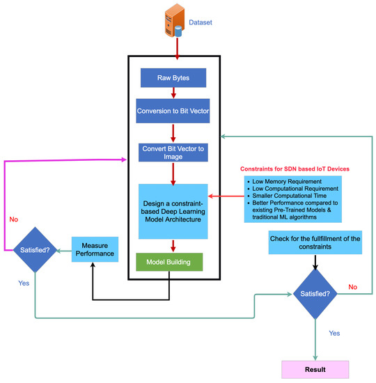
Figure 1. Proposed lightweight model architecture for SDN-IoT orchestrated botnet detection.

3.1. Dataset

The dataset used in this work consists of five classes that were gathered via various IoT device-targeting assaults [39], as shown in Table 1. DoS, DDoS, port scanning, OS fingerprinting, and fuzzing are the five attack types listed in Table 1. The dataset contains six different classes, including the normal classes, with size distributions expressed in megabytes and percentage shares of each class within the dataset. The following is a description of each attack type and additional details of the dataset is given in Table 1 and Table 2.

Table 1. Datasets category and its distribution in size and percentage.

Category	Size (M)	Share in %
Normal	2.67	8.84
DoS	0.49	1.67
DDoS	0.18	0.60
Port Scanning	22.44	74.23
OS and Service Detection	3.39	11.20
Fuzzing	1.05	3.48

Table 2. Dataset features and their description.

Feature Type	Description
srcMAC	Source MAC address
dstMAC	Destination MAC address
srcIP	Source IP address
dstIP	Destination IP address
srcPort	Source port number
dstPort	Destination port number
last_seen	Last time flow was active
Protocol	Textual representation of transaction protocol
proto_number	Numerical representation of protocol
Dur	Flow duration
Mean	Average duration of flows
Stddev	Standard deviation of flows
Min	Minimum duration of flows
Max	Maximum duration of flows
Pkts	Total number of packets matched with flow rules
Bytes	Total number of bytes matched with flow rules
Spkts	Source-to-destination packet count
Dpkts	Destination-to-source packet count
Sbytes	Source-to-destination byte count
Dbytes	Destination-to-source byte count
Srate	Source-to-destination packets per second
Drate	Destination-to-source packets per second
TnBPSrcIP	Total number of bytes per source IP
TnBPDstIP	Total number of bytes per destination IP
TnP_PSrcIP	Total number of packets per source IP
TnP_PDstIP	Total number of packets per destination IP
TnP_PerProto	Total number of packets per protocol
TnP_Per_Dport	Total number of packets per dport
N_IN_Conn_P_SrcIP	Number of inbound connections per source IP
N_IN_Conn_P_DstIP	Number of inbound connections per destination IP
Attack	0 for Normal traffic, 1 for Attack Traffic
Category	Attack category

• Denial of Service: DoS assaults employed the Hping3 tool. Attacks on the server or one of the IoT devices were launched by a single malicious host both with and without the use of faked IP addresses. Using faked IP addresses drains the resources of the controller and switches by causing each attack packet to launch the implementation of a new flow rule. Both SYN flood and UDP flood assaults were carried out. All possible mixtures of the four different packet transmission rates (4000, 6000, 8000, and 10,000) and payload sizes (0, 100, 500, and 1000 bytes) were employed.
• Distributed DoS: One of the most prevalent botnet attacks on IoT networks with SDN support is the DDoS attack. It is an attack that reduces the availability of systems by using their resources. The network’s computational resources are depleted by DDoS attacks, which largely make use of communication protocols that might have been used by authorized users [40]. The identical scenarios that were employed for DoS were also applied to DDoS.
• Port scanning: Port scanning assaults made use of the Nmap tool. The server or one of the IoT devices was the target of an assault initiated by a rogue host. The first 1024 ports are examined by default when using Nmap; however, users can additionally define a range of ports to scan. We checked all of the port numbers and the first 1024 ports (0 to 65,535).
• OS fingerprinting: The OS fingerprinting assault made use of Nmap. In order to find open ports during this assault, the attacker first runs a quick port scan. The attacker then uses these ports to carry out the assault. As a result, we launched an assault that was only directed at the server using one rogue host.
• Attacks that involved fuzzing employed the Boofuzz program. By providing random data until the target fails, this attack aims to identify the victim’s vulnerabilities. By using one of the malicious hosts, we conducted FTP and HTTP fuzzing attacks on the server. For HTTP and FTP connections, our fuzzes produced random values for the input fields and are aware of the anticipated input format. For instance, the random request URL and HTTP version data were fuzzed with HTTP methods like get, head, post, put, delete, connect, options, and trace.

The original dataset is provided in CSV format. However, the study recommends a method in which the model incorporates information from images. Once tabular data has been translated into pictures, the pipeline developed for this project will allow the model to perform categorization. This section will therefore include a description of the technique in Algorithm 1, which is used to transform tabular data into images.

Algorithm 1 Dataset conversion from CSV file format to PNG image format.

1: f = open(x)                         ▹ Read the CSV file (X) 2: Convert (f, delimiter = ’,’)        ▹ Convert the CSV into NumPy array of uint16 3: h, w = rgb565array.shape   ▹ Pick up image dimensions and represent colors in 16 bits 4: numpy.zeros([height, width, 3]) ▹ Make an array of matching for (RGB) with 24-bit colors 5: for row ∈ height do                     ▹ Read each row value 6:   for col ∈ width do                  ▹ Read each column value 7:     rgb565 = rgb565array[row, col]   ▹ Pick up rgb565 value and split into rgb888 8:     red = ((rgb565 $>>$ 11) & 0x1f) $<<$ 3           ▹ Pick the red colors 9:     green = ((rgb565 $>>$ 5 ) & 0x3f) $<<$ 2         ▹ Pick the green colors 10:      blue = ((rgb565) & 0x1f) $<<$ 3    ▹ Pick the rest color which is the blue one 11:      rgb888array[row, col]=red, green, blue         ▹ Populate result array 12:     Save(rgb888array, ‘png’)               ▹ Save result as PNG 13:   end for 14: end for

An array of uint16 values is formed in NumPy after reading the CSV file. Create a Numpy array called rgb888array and then fill it with 0 values. With rows and columns, the array should resemble tabular data, but instead of having just one channel, it should have three: red, green, and blue. Then, while iterating over the rgb888array, the red, green, and blue values are calculated for each element by using the bit shift and AND boolean operation.

By first shifting the binary format left by 11, bitwise ANDing it with hexadecimal 0x 1F, and then shifting the result left by 3, the red channel is determined. By first shifting the binary format left by 5, bitwise ANDing it with hexadecimal 0x3F, and then moving the result left by 2, the green channel is calculated. By bitwise ANDing hexadecimal 0x1F, the blue channel is determined. The output is then shifted left by three bits. The methods in Algorithm 2 will be used to divide the resulting RGB image into 28 × 28-sized images.

Algorithm 2 Split the PNG image into 28 × 28-sized images.

1: $img=read\left(x\right)$                        ▹ read the image (x) from file 2: for $r\in range(0,img.shape[0],28)$do   ▹ read each 28 pixels from the width and store it on r 3:   for $c\in range(0,img.shape[1],28)$ do  ▹ read each 28 pixels from height and store it on c 4:     $write(dst,fname,r+28,c+28)$ ▹ save those pixels on destination folder with filename 5:   end for 6: end for

3.2. Proposed Approach

Object detection [41], time-series data categorization [2,42], and medical image analysis [43] are only a few of the tasks for which a deep learning architecture has been deployed. Most of these designs use models with numerous layers, producing extremely deep models. Wider models are produced when multiscale architecture is employed. Thus, it is crucial to develop a model that accurately reflects how the model operates. The way we construct the deep learning architecture has an impact on the depth/width of the model and the number of parameters that need to be learned. Overfitting can happen when a model has many parameters, while underfitting can happen when a model has few parameters. A gradient vanishing or gradient explosion may also happen when a model’s depth is raised, according to Hanin [44]. As a result, developing a model that perfectly matches the computer resource limitation without compromising classification performance requires a lot of trial and careful thought.

In this study, the SDN dataset is classified into six groups by using a lightweight deep learning architecture. In addition to having a limited number of parameters and requiring little time to run, the model also has a very low memory requirement. These characteristics enable the model to utilize the available computational resource effectively. The lightweight deep learning model’s development method is described in Algorithm 3.

Algorithm 3 Designing a constraint-based lightweight model for IoT devices.

1: _Z: Initialization of hyper-parameters 2: if Number of Convolutional layers is fixed then 3:   Assign an appropriate number of pooling layers 4:   Assign an appropriate number of batch normalization 5:   Assign an appropriate size of a kernel 6:   Build lightweight Model 7: end if 8: Evaluate the appropriateness of lightweight Model 9: if Lightweight Model is not underfit || overfit then 10:   Fine-tune the lightweight-Model 11:   Go to $\_Z$ 12: else 13:   Go to $\_W$ 14: end if 15: $\_W$: Evaluate-performance of lightweight Model 16: if Acc & R & P & F1 ≥ state-of-the-art-result then 17:   Check memory-requirement of lightweight ≤ IoT-devices 18:   Check computational resources are upto-IoT devices 19:   Check computational time is minimum 20:   if Lightweight Model satisfied IoT devices constraints then 21:     Save Model & Model weights 22:     Go to $\_Z$ 23:   end if 24: end if

As presented in Algorithm 3, for less memory space and computational time requirements, three different lightweight architectures (3 × 3, 5 × 5, and 3 × 3–5 × 5 that vary in the size of kernels are proposed, and the 3 × 3–5 × 5 model architecture is depicted in Figure 2. These three models come in two variations, one with batch normalization (BN), and the other without. The proposed 3 × 3 and 5 × 5 architectures with the final BN have Input→CONV2D→ACT→BN→CONV2D→ACT→BN→MAXPOOL→CONV2D→ACT→BN→CONV2D→ACT→BN→GAP→FC layers. The input size is (28, 28, 3), which indicates that the input image contains RGB channels and dimensions of 28 in both width and height. In the 3 × 3 architecture, the size of the feature map after the first, second, third, and fourth Conv2D layers is (14, 14, 16), (12, 12, 16), (9, 9, 32), and (7, 7, 32), respectively. It is (14, 14, 16), (10, 10, 16), (5, 5, 32), and (1, 1, 32) for the 5 × 5 architecture. The difference in the feature map is due to the kernel size difference, which can be calculated with Equation (1).

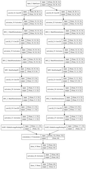
Figure 2. Proposed lightweight deep learning architecture 3 × 3_5 × 5-based convolution without batch normalization before the GAP.

The other proposed modification to this architecture is the removal of BN just before the global average pooling (GAP). The size of the kernels used is the only distinction between the 3 × 3 and 5 × 5 architectures. While a kernel of size 3 is used in the 3 × 3 architecture, a kernel of size 5 is utilized in the 5 × 5 architecture. The third model put forth in this study is a combination of the 3 × 3 and 5 × 5 designs. With the employment of the 3 × 3 and 5 × 5 in parallel, the output from the GAP layer is concatenated to produce 128 features.

The preliminary step in designing a lightweight model is to reduce the number of filters used in the architecture. The first and second CONV2D layer has a filter number of 16, while the third, and fourth CONV2D layers use a filter number of 32. Secondly, MaxPool with two kernel sizes is used only once after the second Conv2D layer. The third method to reduce the required number of parameters is using GAP instead of flattening the layer. For instance, using flatten for the (7, 7, 32) feature map will result in around 1568 output neurons, whereas GAP will only result in 32 neurons, which is significantly less than what would be produced with flattening. One dense layer and the final output layer come after the pooling of the global averages. Since there is no parameter to tune at the global average pooling layer, overfitting is prevented, which gives it an advantage over the flattening layer [45].

The spatial size of the output volume in each layer is calculated by using input size $W1$ ($W2$ will be the output volume), filter size F, stride S, and the amount of zero padding P based on the following Equation (1) as indicated in [46]:

$$W2=\frac{W1-F+2P}{S}+1.$$

(1)

The second convolution layer receives the output of the first convolution as an input. We can calculate the output of the next convolution layer by using the above equation. In the first layer, $W1$ is a 28 × 28 × 3 color image is given to the model, and this spatial volume will be changed after the first convolution. The initial size of filter F is 3 × 3, stride S is 2, and the same padding, based on the above Equation (1). The final result is ((28 − 3 + 2(1))/2) + 1 = 14.5. This is not an integer value so the libraries convert this number into 14. Therefore, the next convolution output value is 14 × 14 × 3,

$$P=\frac{F-1}{2},$$

(2)

where P is padding and F is the filter (kernel).

By using Equation (2), we can determine the kernel or filter size as indicated in Equation (3):

$$F=2P+1.$$

(3)

In the first convolutional layer, we have zero padding of 1 and by using Equation (3) we can get filter size F = 2(1) + 1 = 3. Therefore, the filter is 3 × 3. The reason that we are using a smaller kernel is that if we use a larger kernel, we may start losing details in some smaller features (where 3 × 3 would detect them better). In other words using smaller-sized convolution helps to identify much smaller features that are used to distinguish between the input image and the probability of losing an important feature is much less because the size of our dataset is very small.

3.3. Evaluation Metrics

In a classification task, a true positive (TP) is a pixel that is correctly predicted to belong to the given class based on the ground truth, whereas a true negative (TN) is a pixel that is correctly classified as not belonging to the given class. On the other hand, a false positive (FP) is a result where the model wrongly predicts that a pixel does not belong to a specific class. In addition, a false negative (FN) result occurs when the model forecasts the pixel as wrongly belonging to a particular class. Similar to this, for classification jobs, TP stands for a pixel that is accurately detected as not belonging to the specified class, whereas TN stands for a pixel that is correctly projected to do so based on the ground truth. A false positive (FP), on the other hand, is a result in which the model mistakenly forecasts a pixel as not belonging to a specific class. A false negative (FN) is a result where the model forecasts the class wrongly as belonging to a particular class. Consequently, we defined the following assessment criteria from the literature while keeping in mind various performance indicators utilized in classification.

Accuracy(Acc) gauges a model’s propensity for properly classifying all classes or pixels, whether they are positive or negative:

$$Acc=\frac{TP+TN}{TP+TN+FP+FN}.$$

(4)

Recall (R) measures how accurately the positive predictions made by the machine learning model match the actual data. It provides information on the proportion of classes/pixels that were annotated in our ground truth and were incorporated in the model’s prediction:

$$R=\frac{TN}{TP+FN}.$$

(5)

The frequency with which the model predicts the right class/pixel is measured by precision (P), also known as the positive predictive value (PPV). It accurately reports the percentage of favorable results that the model predicted:

$$P=\frac{TP}{TP+FP}.$$

(6)

The most widely used metric that combines precision and recall is the F1 score. It stands for the two’s harmonic mean:

$$F1score=2\frac{P\ast R}{(P+R)}.$$

(7)

4. Experimental Results and Discussion

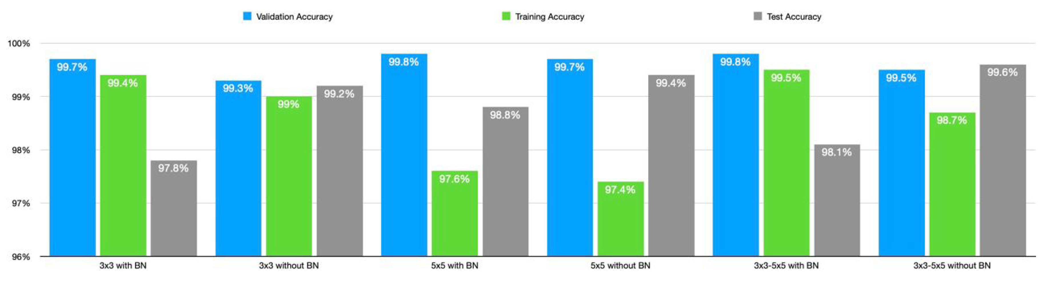
In this section, the results of the 3 × 3, and 5 × 5 CNN models, the fused 3 × 3–5 × 5 CNN models, and other classical machine learning models will be presented and discussed one after the other. The result discussed in this section is obtained with batch size, epoch, and initial learning rate of 32, 150, and 0.001, respectively. Categorical cross-entropy loss is the function used to determine classification loss with the Adam optimizer. The 3 × 3 model achieved 97.8% accuracy, 98% precision, 98% recall, and 0.98 F1 score as presented in Table 3. Its running time, memory requirement, and the number of parameters are 0.113 sec, 235 KB, and 47,622 respectively. Removing the final BN will increase the accuracy to 99.2%. The precision, recall, and F1 score increase to 99%. The other effects of removing the BN layer are a decrease in running time, the number of parameters, and memory requirement. In the same manner, the performance for 5 × 5, and 3 × 3–5 × 5 architectures presented in Table 4 and Table 5 respectively, improves upon removing the final BN layers. The 3 × 3–5 × 5 architecture has identical performance in terms of F1 score, recall, accuracy, and precision. However, its running time and memory requirement increase significantly, although the loss decreases. The comparison of the proposed architecture is found in Figure 3 and Figure 4.

Table 3. The 3 × 3 with and withoutbatch normalization before the global average pooling.

Attack Type/Label	With Batch Normalization before GAP			Without Batch Normalization before GAP
	Precision (%)	Recall (%)	F1 Score	Precision (%)	Recall (%)	F1 Score
DDoS	100	100	1.00	99	100	0.99
DoS	100	98	0.99	100	99	0.99
Fuzzing	100	100	1.00	100	100	1.00
Normal	100	100	1.00	100	100	1.00
OS Fingerprinting	100	88	0.93	100	98	0.99
Port Scanning	89	100	0.94	98	100	0.99
Average	98	98	0.98	99	99	0.99

Table 4. The 5 × 5 with and without batch normalization before the global average pooling.

Attack Type/Label	With Batch Normalization before GAP			Without Batch Normalization before GAP
	Precision (%)	Recall (%)	F1 Score	Precision (%)	Recall (%)	F1 Score
DDoS	98	100	0.99	100	99	0.99
DoS	100	98	0.99	98	100	0.99
Fuzzing	100	100	1.00	100	100	1.00
Normal	100	100	1.00	100	100	1.00
OS Fingerprinting	100	94	0.97	100	97	0.99
Port Scanning	95	100	0.97	97	100	0.99
Average	99	99	0.99	99	99	0.99

Table 5. The 3 × 3–5 × 5 with and without batch normalization before the global average pooling.

Attack Type/Label	With Batch Normalization before GAP			Without Batch Normalization before GAP
	Precision (%)	Recall (%)	F1 Score	Precision (%)	Recall (%)	F1 Score
DDoS	100	98	0.99	100	98	1.00
DoS	98	100	0.99	100	100	1.00
Fuzzing	100	100	1.00	100	100	1.00
Normal	100	100	1.00	100	100	1.00
OS Fingerprinting	100	80	0.89	100	94	0.97
Port Scanning	84	100	0.91	95	100	0.97
Average	97	96	0.96	99	99	0.99

Figure 3. Comparison of the three proposed lightweight models in terms of accuracy.

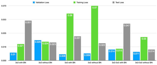
Figure 4. Comparison of the three proposed lightweight models in terms of loss.

In comparison to the one with batch normalization, the performance of 3 × 3 without BN is better. With F1 scores of 0.93 and 0.94 for the OS fingerprinting, and port scanning attack and 0.99 for both classes in the network without BN, there has been a significant increase in the detection of these attacks while removing the BN. For the network architecture of 5 × 5, and 3 × 3–5 × 5, the detection of OS fingerprinting and port scanning attacks follows the patterns we saw in the 3 × 3 architecture. Removal of the BN has also increased the detection of these attacks, with F1 scores of 0.97 for attack detection in the network with BN and 0.99 for both in the network without BN. The 5 × 5 architecture has the lowest test loss of all of the suggested architectures with a loss of 0.008, and the 3 × 3 architecture comes in second with a loss of 0.01 points. The 3 × 3–5 × 5 architecture’s loss, however, has the highest value at 0.011.

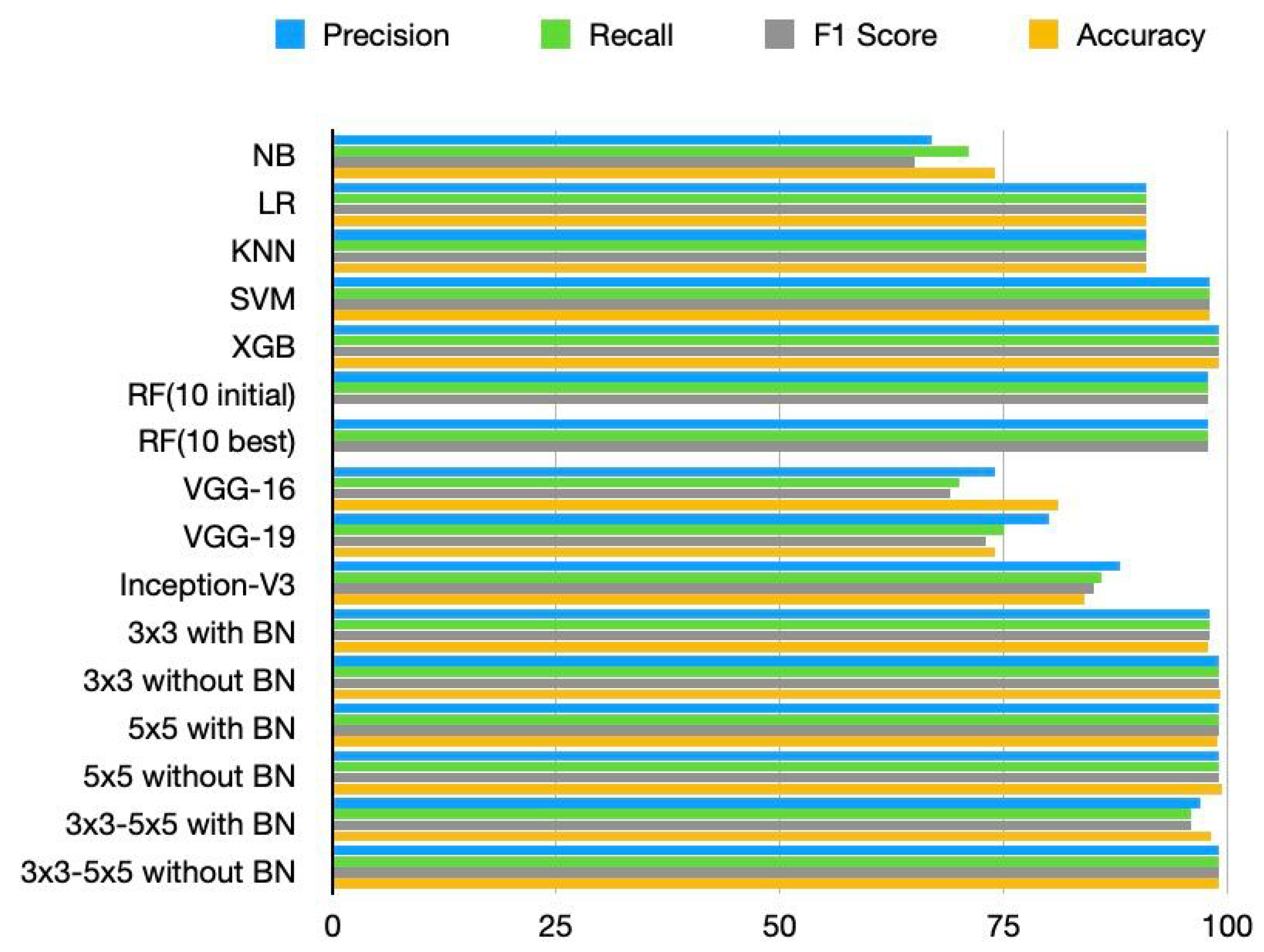
We found that the performance of our proposed model has improved in terms of computational resource requirements and classification accuracy when compared to the performance of the current state-of-the-art models. While SVM and XG-Boost perform similarly to our method in terms of accuracy, the proposed CNN models perform significantly better in terms of running time and memory requirements. NB, LR, and KNN have the shortest running times, as shown in Table 6; however, they perform poorly in terms of classification when compared to the suggested model. Figure 5 communicates the running time result of each model visually, and we can see that the proposed model achieves a lower running time compared to SVM and XG-boost. Similarly, from Figure 6 we can observe that the precision, recall, F1 score, and accuracy of the proposed models are better compared to the existing model.

Table 6. Comparison of the proposed approach with previous works in terms of size, running time, and a number of parameters.

Model Architecture	Loss	Size (KB)	Number of Parameters	Time (Milliseconds)
NB	-	3.65	-	0.0010
LR	-	2.29	-	0.0030
KNN	-	327	-	0.0030
SVM	-	6000	-	1.500
XGB	-	2700	-	0.140
RF (10 initially selected features)	-	2700	-	0.140
RF (10 best-selected features)	-	2700	-	0.140
VGG-16	-	512.43 MB	in millions	in minutes
VGG-19	-	542.34 MB	in millions	in minutes
Inception-V3	-	91.55 MB	in millions	in minutes
3 × 3 with_BN	0.051	122	19542	0.1130
3 × 3 withou_ BN	0.023	118	19414	0.1080
5 × 5 with_BN	0.031	240	48982	0.1080
5 × 5 without_BN	0.022	237	48854	0.1073
3 × 3_5 × 5 with_BN	0.011	349	68070	0.1230
3 × 3_5 × 5 without_BN	0.014	342	67814	0.1170

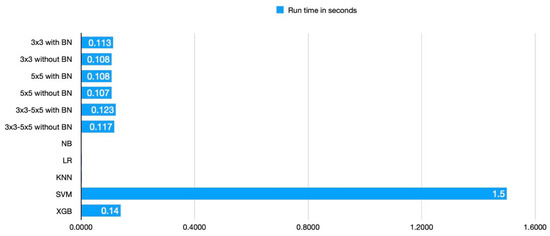
Figure 5. Comparison of models in terms of run time.

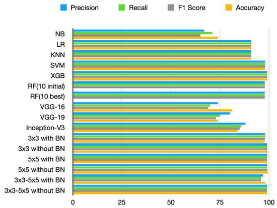
Figure 6. Comparison of models in terms of accuracy, precision, recall, and F1 score.

As presented in Table 6, our proposed model has fewer parameters compared to pre-trained models and less model size compared to both pre-trained models and traditional machine learning techniques, which makes the proposed model be installed and perform well in low computational resource machines like IoT devices. Similarly, from the experimental result, we found that our proposed model outperforms both pre-trained models and traditional machine learning algorithms in terms of precision, recall, F1 score and accuracy as indicated in Table 7. Besides, the proposed approach can identify any malware on the devices in milliseconds.

Table 7. Comparison of the proposed method with previous work on SDN datasets for 10-IoT devices.

Method	Precision (%)	Recall (%)	F1 Score	Accuracy (%)
NB	67	71	0.65	74
LR	91	91	0.91	91
KNN	91	91	0.91	91
SVM	98	98	0.98	98
XGB	99	99	0.99	99
RF (10 initially selected features)	97.86	97.87	0.9786	-
RF (10 best selected features)	97.82	97.82	0.9781	-
VGG-16	74	70	0.69	81
VGG-19	80	75	0.73	74
Inception-V3	88	86	0.85	84.1
3 × 3 with_BN	98	98	0.98	97.8
3 × 3 withou_ BN	99	99	0.99	99.2
5 × 5 with_ BN	99	99	0.99	98.8
5 × 5 without_ BN	99	99	0.99	99.4
3 × 3—5 × 5 with_ BN	97	96	0.96	98.1
3 × 3–5 × 5 without_ BN	99	99	0.99	99.0

5. Conclusions

Beyond conventional computing systems, the SDN and IoT have made it feasible to connect to a variety of sensors and electronic equipment. Such botnet assaults as DoS, DDoS, fuzzing, Boofuzz, OS fingerprinting, port scanning, etc. still pose a threat to these networks. These attacks may disrupt a number of economic sectors, and on rare occasions they may even cause irreversible damage. Attacks can be detected quickly via computer-assisted botnet detection, which can help to mitigate their consequences. For real-time botnet attack detection, a number of conventional machine learning techniques have been put forth and assessed. Nevertheless, the majority of these methods necessitate intensive feature engineering, which makes them dependent on feature extraction from known malware signatures both during training and after deployment. Therefore, it is still crucial to find solutions for the crucial challenges of quick detection, ongoing monitoring, and adaptability to new threats. It is not a viable solution for deploying models on IoT devices because it also uses significantly more processing resources and takes much longer to compute. If there is any amount of training data available, deep learning models are well known for their robustness in the classification task and their ability to address these problems. They also do not need feature engineering because they can extract patterns on their own without assistance from a human. We therefore suggested lightweight deep learning in this study for the identification of five botnet attacks: DoS, DDoS, fuzzing, Boofuzz, OS fingerprinting, and port scanning. The lightweight model is achieved by carefully designing a deep learning model architecture with four convolutional layers, a few filters, and global average pooling thereafter. The proposed method offers increased classification performance, a short operating time, and reduced memory needs. As future research work, we recommend focusing on enhancing the model’s interpretability and explainability to pinpoint crucial features that significantly influence model predictions.

References

- Wube, H.D.; Esubalew, S.Z.; Weldesellasie, F.F.; Debelee, T.G. Text-Based Chatbot in Financial Sector: A Systematic Literature Review. Data Sci. Financ. Econ. 2022, 2, 232–259. [Google Scholar] [CrossRef]
- Feyisa, D.W.; Debelee, T.G.; Ayano, Y.M.; Kebede, S.R.; Assore, T.F. Lightweight Multireceptive Field CNN for 12-Lead ECG Signal Classification. Comput. Intell. Neurosci. 2022, 2022, 8413294. [Google Scholar] [CrossRef] [PubMed]
- Afework, Y.K.; Debelee, T.G. Detection of bacterial wilt on enset crop using deep learning approach. Int. J. Eng. Res. Afr. 2020, 51, 131–146. [Google Scholar] [CrossRef]
- Biratu, E.S.; Schwenker, F.; Ayano, Y.M.; Debelee, T.G. A survey of brain tumor segmentation and classification algorithms. J. Imaging 2021, 7, 179. [Google Scholar] [CrossRef]
- Rufo, D.D.; Debelee, T.G.; Ibenthal, A.; Negera, W.G. Diagnosis of diabetes mellitus using gradient boosting machine (LightGBM). Diagnostics 2021, 11, 1714. [Google Scholar] [CrossRef]
- Waldamichael, F.G.; Debelee, T.G.; Ayano, Y.M. Coffee disease detection using a robust HSV color-based segmentation and transfer learning for use on smartphones. Int. J. Intell. Syst. 2021, 37, 4967–4993. [Google Scholar] [CrossRef]
- Li, S.; Xu, L.D.; Zhao, S. The internet of things: A survey. Inf. Syst. Front. 2014, 17, 243–259. [Google Scholar] [CrossRef]
- Al-Rushdan, H.; Shurman, M.M.; Alnabelsi, S.H.; Althebyan, Q. Zero-Day Attack Detection and Prevention in Software-Defined Networks. In Proceedings of the 2019 International Arab Conference on Information Technology (ACIT), Al Ain, United Arab Emirates, 3–5 December 2019; pp. 278–282. [Google Scholar]
- Negera, W.G.; Schwenker, F.; Debelee, T.G.; Melaku, H.M.; Ayano, Y.M. Review of Botnet Attack Detection in SDN-Enabled IoT Using Machine Learning. Sensors 2022, 22, 9837. [Google Scholar] [CrossRef] [PubMed]
- Product Manager: Cyber Security in 2020 and beyond. Available online: https://outpost24.com/blog/Cyber-Security-in-2020-and-beyond (accessed on 26 December 2022).
- Pandey, A.K.; Tripathi, A.K.; Kapil, G.; Singh, V.; Khan, M.W.; Agrawal, A.; Kumar, R.; Khan, R.A. Trends in Malware Attacks; IGI Global: Hershey, PA, USA, 2020; pp. 47–60. [Google Scholar] [CrossRef]
- Suresh, P.; Daniel, J.V.; Parthasarathy, V.; Aswathy, R. A state-of-the-art review on the Internet of Things (IoT) history, technology, and fields of deployment. In Proceedings of the 2014 International Conference on Science Engineering and Management Research (ICSEMR), Chennai, India, 27–29 November 2014; pp. 1–8. [Google Scholar]
- International Telecommunication Union. ITU Internet Report 2005: The Internet of Things; ITU: Geneva, Switzerland, 2005; Available online: http://www.itu.int/osg/spu/publications/internetofthings/ (accessed on 14 October 2022).
- Acarali, D.; Rajarajan, M.; Komninos, N.; Zarpelão, B.B. Modelling the Spread of Botnet Malware in IoT-Based Wireless Sensor Networks. Secur. Commun. Netw. 2019, 2019, 3745619. [Google Scholar] [CrossRef]
- Liaqat, S.; Akhunzada, A.; Shaikh, F.S.; Giannetsos, A.; Jan, M.A. SDN orchestration to combat evolving cyber threats in Internet of Medical Things (IoMT). Comput. Commun. 2020, 160, 697–705. [Google Scholar] [CrossRef]
- Thomas, D.; Nadeau, K.G. Sdn: Software Defined Networks: An Authoritative Review of Network Programmability Technologies; Oreilly Media: Sebastopol, CA, USA, 2013. [Google Scholar]
- Sarker, I.H.; Kayes, A.S.M.; Badsha, S.; Alqahtani, H.; Watters, P.; Ng, A. Cybersecurity data science: An overview from machine learning perspective. J. Big Data 2020, 7, 1–29. [Google Scholar] [CrossRef]
- Sethi, K.; Kumar, R.; Sethi, L.; Bera, P.; Patra, P.K. A Novel Machine Learning Based Malware Detection and Classification Framework. In Proceedings of the 2019 International Conference on Cyber Security and Protection of Digital Services (Cyber Security, Oxford, UK, 3–4 June 2019. [Google Scholar] [CrossRef]
- Gibert, D.; Mateu, C.; Planes, J. The rise of machine learning for detection and classification of malware: Research developments, trends and challenges. J. Netw. Comput. Appl. 2020, 153, 102526. [Google Scholar] [CrossRef]
- Amin, F.; Abbasi, R.; Mateen, A.; Ali Abid, M.; Khan, S. A Step toward Next-Generation Advancements in the Internet of Things Technologies. Sensors 2022, 22, 8072. [Google Scholar] [CrossRef] [PubMed]
- Li, Y.; Su, X.; Ding, A.Y.; Lindgren, A.; Liu, X.; Prehofer, C.; Riekki, J.; Rahmani, R.; Tarkoma, S.; Hui, P. Enhancing the internet of things with knowledge-driven software-defined networking technology: Future perspectives. Sensors 2020, 20, 3459. [Google Scholar] [CrossRef] [PubMed]
- Sung, A.; Abraham, A.; Mukkamala, S. Cyber-Security Challenges; Auerbach Publications: London, UK, 2005; pp. 125–164. [Google Scholar] [CrossRef]
- Sun, N.; Zhang, J.; Rimba, P.; Gao, S.; Zhang, L.Y.; Xiang, Y. Data-Driven Cybersecurity Incident Prediction: A Survey. IEEE Commun. Surv. Tutor. 2019, 21, 1744–1772. [Google Scholar] [CrossRef]
- McIntosh, T.; Jang-Jaccard, J.; Watters, P.; Susnjak, T. The Inadequacy of Entropy-Based Ransomware Detection; Springer: Berlin/Heidelberg, Germany, 2019; pp. 181–189. [Google Scholar] [CrossRef]
- Jang-Jaccard, J.; Nepal, S. A survey of emerging threats in cybersecurity. J. Comput. Syst. Sci. 2014, 80, 973–993. [Google Scholar] [CrossRef]
- Sarica, A.K.; Angin, P. Explainable security in SDN-based IoT networks. Sensors 2020, 20, 7326. [Google Scholar] [CrossRef]
- Park, Y.; Kengalahalli, N.V.; Chang, S.Y. Distributed security network functions against botnet attacks in software-defined networks. In Proceedings of the 2018 IEEE Conference on Network Function Virtualization and Software Defined Networks (NFV-SDN), Verona, Italy, 27–29 November 2018; pp. 1–7. [Google Scholar]
- Thorat, P.; Dubey, N.K. SDN-based machine learning powered alarm manager for mitigating the traffic spikes at the IoT gateways. In Proceedings of the 2020 IEEE International Conference on Electronics, Computing and Communication Technologies (CONECCT), Bangalore, India, 2–4 July 2020; pp. 1–6. [Google Scholar]
- Alamri, H.A.; Thayananthan, V. Bandwidth control mechanism and extreme gradient boosting algorithm for protecting software-defined networks against DDoS attacks. IEEE Access 2020, 8, 194269–194288. [Google Scholar] [CrossRef]
- Swami, R.; Dave, M.; Ranga, V. Detection and analysis of TCP-SYN DDoS attack in software-defined networking. Wirel. Pers. Commun. 2021, 118, 2295–2317. [Google Scholar] [CrossRef]
- Dake, D.K.; Gadze, J.D.; Klogo, G.S.; Nunoo-Mensah, H. Multi-agent reinforcement learning framework in sdn-iot for transient load detection and prevention. Technologies 2021, 9, 44. [Google Scholar] [CrossRef]
- Uğurlu, M.; Doğru, İ.A. A survey on deep learning based intrusion detection system. In Proceedings of the 2019 4th International Conference on Computer Science and Engineering (UBMK), Samsun, Turkey, 11–15 September 2019; pp. 223–228. [Google Scholar]
- Tang, T.A.; Mhamdi, L.; McLernon, D.; Zaidi, S.A.R.; Ghogho, M. Deep learning approach for network intrusion detection in software defined networking. In Proceedings of the 2016 international conference on wireless networks and mobile communications (WINCOM), Fez, Morocco, 26–29 October 2016; pp. 258–263. [Google Scholar]
- Narayanadoss, A.R.; Truong-Huu, T.; Mohan, P.M.; Gurusamy, M. Crossfire attack detection using deep learning in software defined its networks. In Proceedings of the 2019 IEEE 89th Vehicular Technology Conference (VTC2019-Spring), Kuala Lumpur, Malaysia, 28 April–1 May 2019; pp. 1–6. [Google Scholar]
- Al-Abassi, A.; Karimipour, H.; Dehghantanha, A.; Parizi, R.M. An ensemble deep learning-based cyber-attack detection in industrial control system. IEEE Access 2020, 8, 83965–83973. [Google Scholar] [CrossRef]
- de Assis, M.V.; Carvalho, L.F.; Rodrigues, J.J.; Lloret, J.; Proença Jr, M.L. Near real-time security system applied to SDN environments in IoT networks using convolutional neural network. Comput. Electr. Eng. 2020, 86, 106738. [Google Scholar] [CrossRef]
- Ullah, I.; Raza, B.; Ali, S.; Abbasi, I.A.; Baseer, S.; Irshad, A. Software defined network enabled fog-to-things hybrid deep learning driven cyber threat detection system. Secur. Commun. Netw. 2021, 2021, 1–15. [Google Scholar] [CrossRef]
- Khan, S.; Akhunzada, A. A hybrid DL-driven intelligent SDN-enabled malware detection framework for Internet of Medical Things (IoMT). Comput. Commun. 2021, 170, 209–216. [Google Scholar] [CrossRef]
- AlperKaan35/SDN-Dataset. Available online: https://github.com/AlperKaan35/SDN-Dataset (accessed on 1 July 2021).
- Wang, S.; Gomez, K.; Sithamparanathan, K.; Asghar, M.R.; Russello, G.; Zanna, P. Mitigating ddos attacks in sdn-based iot networks leveraging secure control and data plane algorithm. Appl. Sci. 2021, 11, 929. [Google Scholar] [CrossRef]
- Guo, J.M.; Yang, J.S.; Seshathiri, S.; Wu, H.W. A light-weight CNN for object detection with sparse model and knowledge distillation. Electronics 2022, 11, 575. [Google Scholar] [CrossRef]
- Ayano, Y.M.; Schwenker, F.; Dufera, B.D.; Debelee, T.G. Interpretable Machine Learning Techniques in ECG-Based Heart Disease Classification: A Systematic Review. Diagnostics 2022, 13, 111. [Google Scholar] [CrossRef] [PubMed]
- Abdou, M.A. Literature review: Efficient deep neural networks techniques for medical image analysis. Neural Comput. Appl. 2022, 34, 5791–5812. [Google Scholar] [CrossRef]
- Hanin, B. Which neural net architectures give rise to exploding and vanishing gradients? Adv. Neural Inf. Process. Syst. 2018, 31. [Google Scholar] [CrossRef]
- Lin, M.; Chen, Q.; Yan, S. Network in network. arXiv 2013, arXiv:1312.4400. [Google Scholar]
- Dumoulin, V.; Visin, F. A guide to convolution arithmetic for deep learning. arXiv 2018, arXiv:1603.07285v2. [Google Scholar]
Disclaimer/Publisher’s Note: The statements, opinions and data contained in all publications are solely those of the individual author(s) and contributor(s) and not of MDPI and/or the editor(s). MDPI and/or the editor(s) disclaim responsibility for any injury to people or property resulting from any ideas, methods, instructions or products referred to in the content. |
© 2023 by the authors. Licensee MDPI, Basel, Switzerland. This article is an open access article distributed under the terms and conditions of the Creative Commons Attribution (CC BY) license (https://creativecommons.org/licenses/by/4.0/).