Featured Application
The work in this paper can be used as a scheme for cross-sectional profile fitting and geometry dimension measurement for single-pass multilayer welding methods and can be used as an aid in studies of welding parameter optimization, weld shape prediction, and welding mechanism.
Abstract
A visual measurement method based on a key point detection network is proposed for the difficulty of fitting the cross-sectional profile of ultra-narrow gap welds and the low efficiency and accuracy of manual measurement of geometric parameters. First, the HRnet (High-Resolution Net) key point detection algorithm was used to train the feature point detection model, and 18 profile feature points in a “measurement unit” were extracted. Secondly, the feature point coordinates are transformed from the image coordinate system to the weld coordinate system, and the weld profiles are fitted by the least squares method. Finally, the measurement system is calibrated with a coplanar linear calibration algorithm to perform pixel distance to actual distance conversion for quantitative detection of geometric dimensions. The experimental results show that the accuracy of the proposed method for key point localization is 95.6%, the mean value of the coefficient of determination R-square for curve fitting is greater than 94%, the absolute error of measurement is between 0.06 and 0.15 mm, and the relative error is between 1.27% and 3.12%. The measurement results are more reliable, and the efficiency is significantly improved compared to manual measurement.
1. Introduction
Ultra-narrow gap welding is a highly efficient, low heat input single-pass multilayer welding method applied to narrow gap thick plate welding [1,2]. The shape and geometric dimension of the weld cross-section can reflect the welded joint’s quality and directly represent the weld result, which shows a highly nonlinear relationship with the welding process parameters [3,4,5]. With the development of machine learning, objective optimization algorithms and neural network algorithms are widely used in studies of welding process parameter optimization, weld shape prediction, and online forecasting of weld quality, etc. [6,7,8]. Training these models requires a large amount of cross-sectional shape data, and their detection accuracy and efficiency are key to the above studies.
The current domestic and international research on weld cross-section shape can be summarized into two categories: the first category is curve fitting of the weld profile to establish a geometric model to describe the weld shape as a whole, where the key step is the extraction of the weld profile feature points. Sun et al. first manually located three key points on the weld and then extracted the coordinates of other feature points of the weld using the Hermite interpolation method, followed by the geometric model of the weld profile using segmented least squares fitting [9]. Zou Yuanyuan et al. extracted the weld profile feature points using the image processing method of edge detection, and exponential and Gaussian functions were fitted to the upper and lower edges of the weld to obtain the geometric model of the weld profile [10]. Wang et al. manually took a pole point at certain polar angle intervals on the weld profile based on the polar coordinate system. They used the method of cubic interpolation with MATLAB to fit the weld cross-sectional profile [11]. Researchers commonly use the analytic coefficients of the geometric model as output variables of the weld profile prediction model for weld profile prediction. The second type is the measurement of geometric dimensions such as weld fusion width, fusion depth, and weld height to describe the weld shape quantitatively. The measurement is mainly performed manually using measuring instruments directly, or manually using measurement software for image measurement. Gao et al. manually measured the weld cross-sectional fusion width and fusion depth using calipers during parametric optimization modeling [12]. Yu J et al. used Image-pro software to measure the weld cross-section’s fusion width and weld height during the optimization of the laser-arc composite welding process parameters [13].
When extracting the ultra-narrow gap single-layer weld profile, the efficiency of manually locating individual points and then using the interpolation method to extract feature points is low. At the same time, the edge of the weld profile is blurred, and the error of taking feature points by the edge detection method is also relatively large. When measuring geometric dimensions, adjacent welds are fused, and the weld fusion depth measurement points and weld height measurement points cannot be directly observed, but can only be located by experience, and the measurement accuracy is limited by the experience of the measurement personnel, and the efficiency is not high when processing a large amount of data. Currently, with the development of deep learning, the emergence of the key point detection model provides a new idea for the efficient extraction of weld profile feature points and now has a wide range of applications in industrial image processing. Wang et al. proposed a single tillers rice key point prediction and skeleton extraction method based on an hourglass network model to obtain phenotypic parameters, such as spike length, by detecting rice key points to speed up rice breeding [14]. Liu et al. proposed a semi-supervised skeletal image key point detection framework to accurately extract the key point locations in human hip joints to measure anatomical parameters [15].
This paper proposes a method for detecting weld cross-sectional profiles by integrating computer vision and deep learning. First, the key point detection algorithm HRnet is used to extract 18 feature points on a weld “measurement unit”, and least squares is used to fit the feature points to obtain the geometric model of the weld profile. Then, the geometric relationship of the profile is established by using the characteristics of the adjacent weld channel fusion to locate the pixel coordinates of the measurement points of the geometric parameters of the weld, and to find the geometric parameter pixel distances. Finally, the measurement system is calibrated with a coplanar linear calibration algorithm, and the pixel distance to actual distance conversion is performed to achieve quantitative detection of the bottom sidewall fusion width, maximum sidewall fusion width, weld height, and fusion depth for ultra-narrow gap welding, increasing the measurement rate by order of magnitude. The method can be applied to the field of welding cross-sectional shape inspection for single-pass multilayer welding methods.
2. General Scheme of the Detection System
2.1. Ultra-Narrow Gap Welding Method
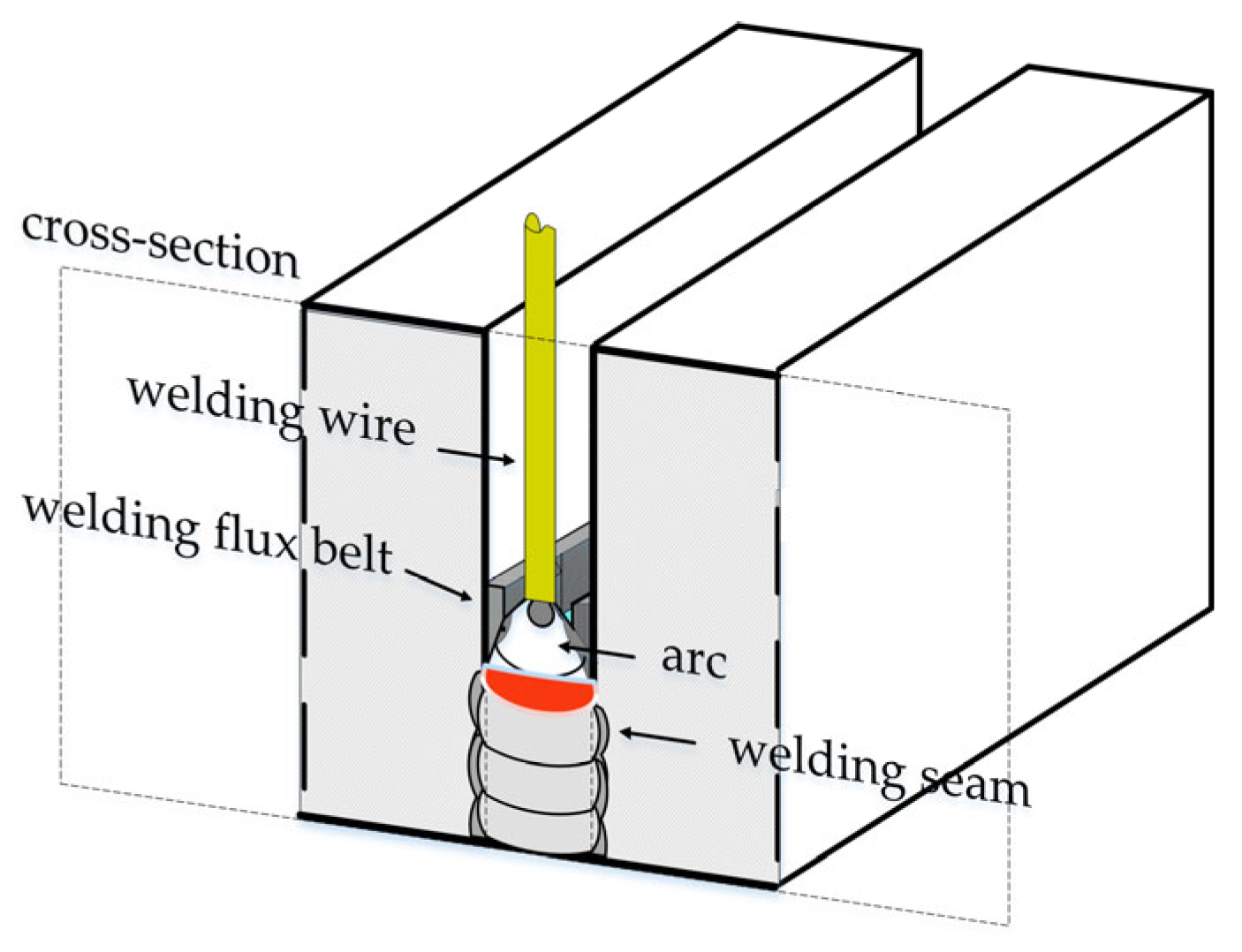
The ultra-narrow gap welding principle is shown in Figure 1. In a 4–6 mm wide “I” shaped straight groove, the flux sheet is used to restrain and regulate the arc to heat and melt both walls simultaneously and the bottom of the weld surface, resulting in a single-pass formation of each layer of the weld, with a smaller weld volume and lower linear energy than conventional arc welding, and good mechanical properties of the joint. The weld cross-sectional shape parameters are the key variables of the method for parameter optimization and quality online prediction studies.

Figure 1.
Ultra-narrow gap welding principle diagram.
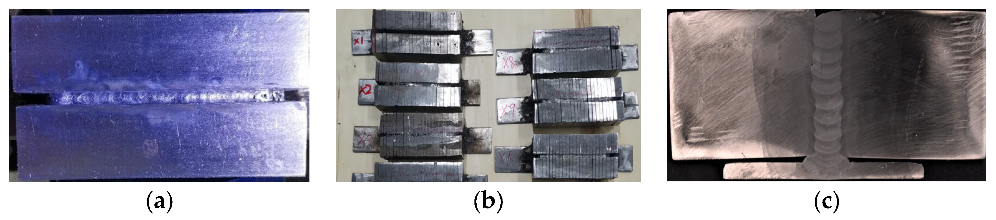
A large number of welding tests were carried out according to the welding parameters in Table 1, and welded specimens were obtained as shown in Figure 2a. Then, it was sliced using a sawing machine as shown in Figure 2b; finally, the slicing samples were ground and polished using 200, 400, and 600 mesh grinding wheels, and a 4% nitric acid alcohol solution was modulated to etch the slicing samples, while anhydrous ethanol was used to clean and dry the samples to obtain the weld cross-sectional shape as shown in Figure 2c.

Table 1.
Welding parameters range.
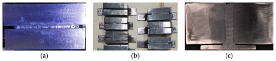
Figure 2.
Description of the process of obtaining weld cross-section slices: (a) welding specimen; (b) specimens after slicing; (c) specimens after slicing and etching.
2.2. Measurement Parameters
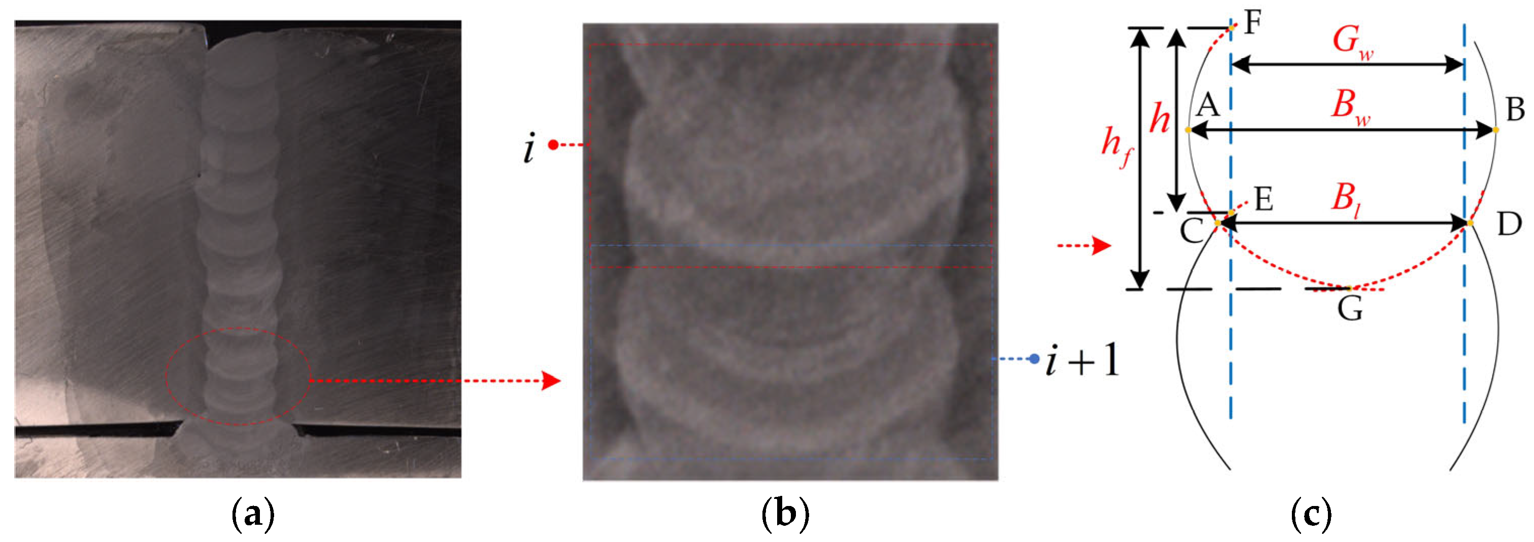
Figure 3a shows the weld cross-sectional shape of the welded specimen. The dividing line between the weld and the base material is called the fusion line, where a pair of fusion lines represent a layer of weld, and the specimen contains a total of ten layers. As shown in Figure 3b, any two adjacent welds are defined as a “Measurement unit” consisting of the and welds, and the measurement method is described in this figure. Figure 3c is a schematic diagram of the cross-sectional shape characteristics dimensions, where is the groove width, a known parameter; is the bottom sidewall fusion width, and is the distance between a pair of fusion line endpoints, and is a critical dimension to determine the fusion of the sidewall and sidewall root; is the maximum fusion width of the weld, and is the distance between maximum points A and B of a pair of fusion lines, which indicates the degree of fusion of the weld and the base material; is the weld height, which is the distance between the intersection point E and F of the adjacent fusion line extension line and the groove width schematic line; is the weld fusion depth, and the distance from the fusion line extension line intersection point G point to F point is the maximum distance between the current weld surface and the fusion area of the current weld and the previous weld.
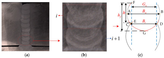
Figure 3.
Illustration of weld image and geometric dimensions to be measured: (a) cross-sectional image of a welded specimen; (b) a “measurement unit” image; (c) geometric dimension diagram.
2.3. Measurement Systems
The measurement system, shown in step A of Figure 4, consists of an industrial vision camera frame and a vision measurement unit, which includes a CMOS image sensor with a resolution of 5496 × 3672 and an image element size of 2.4 μm, and a high-temperature ceramic checkerboard calibration plate with an accuracy of 0.001 mm.
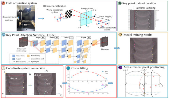
Figure 4.
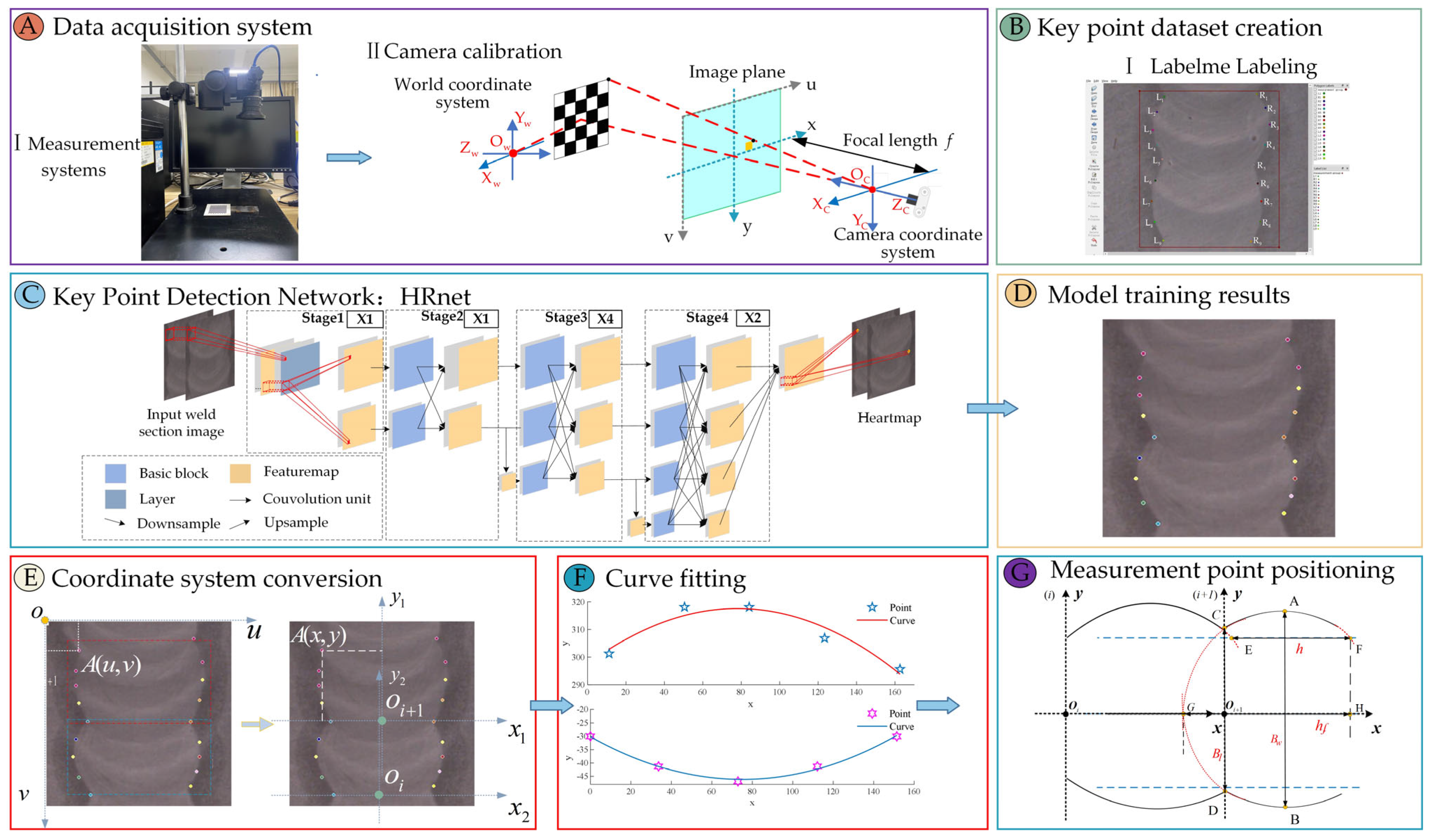
Flow chart of weld cross-section shape detection.
2.4. Measurement Principle
The measurement steps of the proposed method are shown in Figure 4. First, the weld shape is collected using the measurement system, and the camera is calibrated using the coplanar linear camera calibration method, as shown in step (A). Next, 18 feature points of the “measurement unit” are defined. A fusion line corresponds to five feature points to build the key point detection data set and train the key point detection network HRnet to realize the feature point localization of the “measurement unit,” as shown in steps (B), (C), and (D). Then, the coordinates of the key points are transformed to the weld coordinate system, and the five key points are fitted with the least squares method to obtain the geometric model of the fusion line, as shown in steps (E) and (F). Finally, the fitted curves are placed in the same coordinate system, and the coordinates of the key measurement points are derived using geometric relationships to obtain the dimensions of the shape parameters, as shown in step (G).
3. Profile Fitting and Geometric Modeling
3.1. “Measurement Unit” Key Point Detection
3.1.1. “Measurement Unit” Key Point Dataset Creation
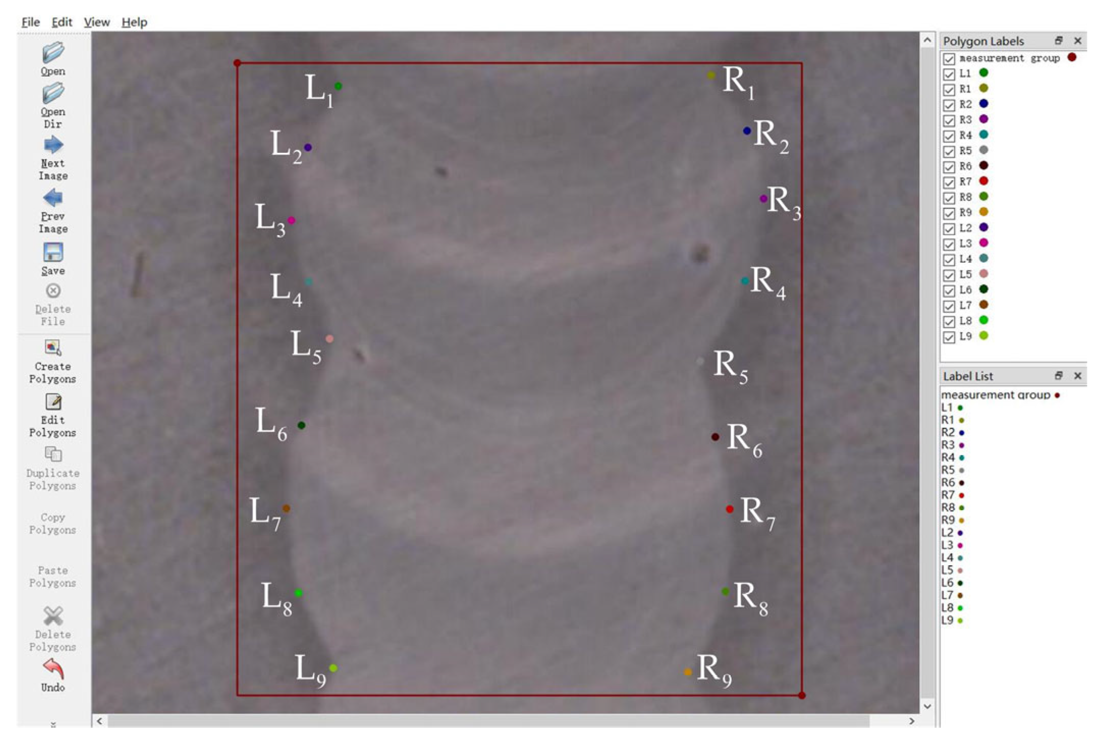
In this paper, the key point data set of the ultra-narrow gap welding “measurement unit” is established, as shown in Table 2, and the “measurement unit” is divided into four areas according to the location of the fusion line; each site contains five key points, where and are the common points of adjacent welding channels, a total of eighteen key points are labeled, and the labeling results are shown in Figure 5.
Table 2.
Definition of key points of the “Measurement unit”.
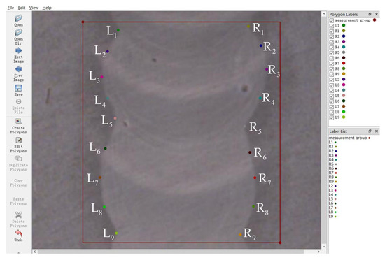
Figure 5.
“Measurement unit” key point labeling diagram.
Because the detection object is a single target and the position of the same key point is similar in the different “measurement unit” images, a good training effect can be achieved with small sample data. A total of 400 “measurement unit” images are labeled in this paper, which are randomly divided into training and validation sets according to the ratio of 8:2. Key point annotation is performed on the Labelme platform, an image annotation tool developed by the Computer Science and Artificial Intelligence Laboratory (CSAIL) at Massachusetts Institute of Technology (MIT), which allows people to create custom annotation tasks or perform image annotation. After the annotation is completed, the labels obtained from the annotation in JSON file format are transformed into the COCO2017 format suitable for HRnet network training.
3.1.2. HRnet Network Structure
HRNet is a key point detection network for 2D human pose estimation based on the heatmap approach, which can better extract multi-resolution features of the input image and has a powerful feature representation capability [16,17,18]. The layout of the 18 key points of the “measurement unit” is centrosymmetric with the layout of the human body key points, which has excellent similarity; so, the HRNet network is used as the feature point detection network, and its network structure is shown in Figure 6.
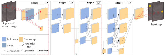
Figure 6.
HRnet network structure diagram.
After inputting the “measurement unit” image into the network, the number of channels is first adjusted by four times downsampling through the convolution layer, then through the Layer layer, which consists of repeated stacks of Bottleneck modules, and then through four stage layers for information fusion. Taking Stage 3 as an example, for each branch, the information on different scales is first fused by four Basic Blocks composed of residual blocks, and the output on each branch is obtained by combining the output on all components after Upsamp or Downsamp. Finally, Stage 4 only outputs the output of the downsampled four times branch, and after a 1 × 1 convolutional layer to extract features, the heatmap of each key point on the fusion line is obtained to achieve key point detection.
3.2. Coordinate System Transformation and Curve Fitting
3.2.1. Coordinate System Transformation
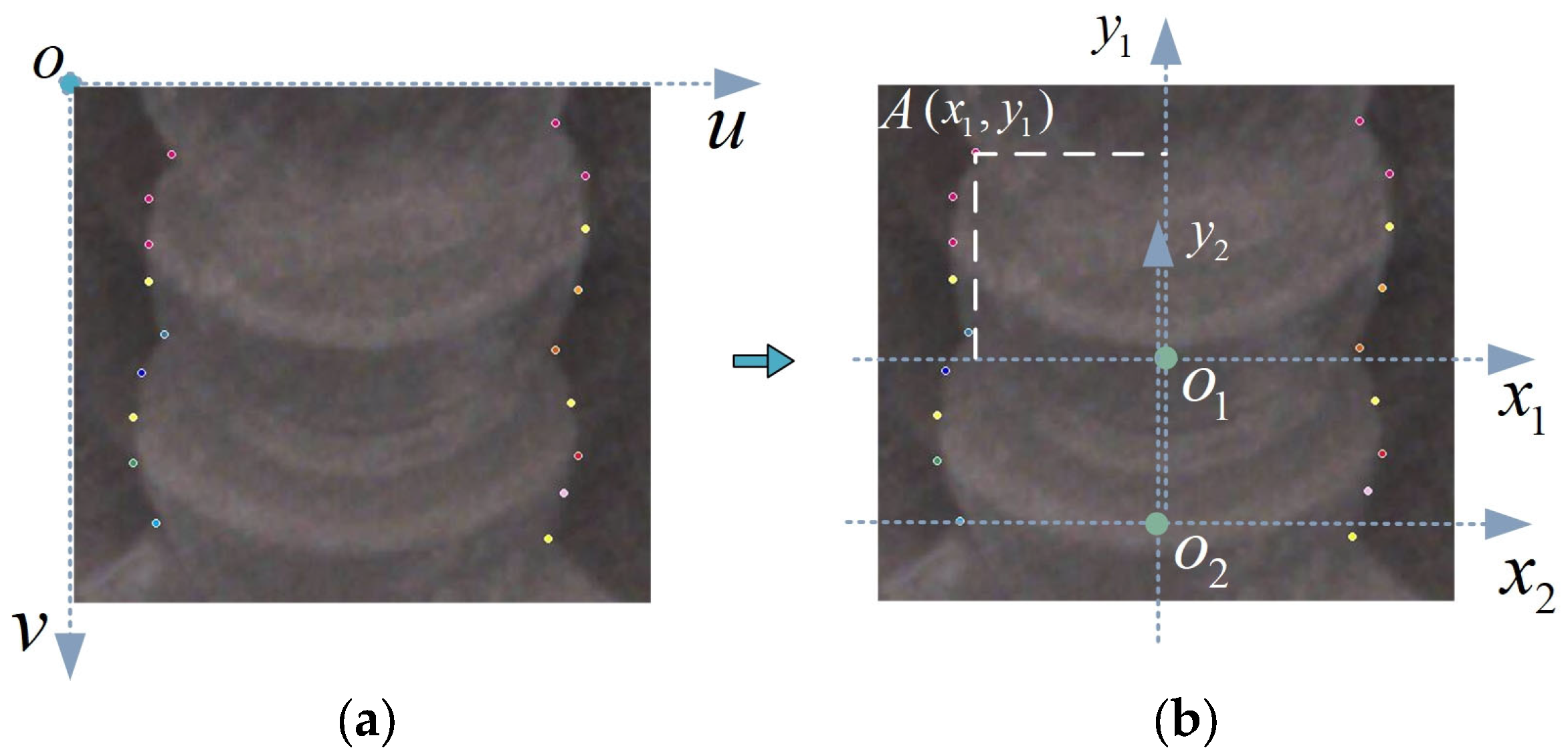
After performing key point detection, the feature points are displayed within the pixel coordinate system with the coordinate origin in the upper left corner of the image, the u-axis along the image width direction, and the v-axis along the image height direction, as shown in Figure 7a. To facilitate fitting the fusion line, the key point coordinates need to be converted to a weld coordinate system with the origin at the center of the weld path, as shown in Figure 7b. The procedure for locating the origin coordinates and transforming the key point coordinates for the weld is as follows:
- The coordinate sequence of the feature points detected by the HRnet network in the pixel coordinate system is .
- The horizontal coordinates of the five groups of feature points are differenced and averaged to obtain the horizontal coordinates of the origin in the pixel coordinate system as:
- The maximum value of the vertical coordinate of the 5 groups of key points is calculated, and the vertical coordinate of the origin in the pixel coordinate system is obtained as
- The horizontal and vertical coordinates of the feature point in the pixel coordinate system are subtracted from the horizontal and vertical coordinates of the point to obtain the horizontal coordinates , and vertical coordinates of the feature point in the weld coordinate system. The coordinates of point A in the pixel coordinate system are ; the coordinates of the weld coordinate system are .
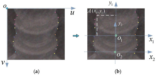
Figure 7.
Diagram of coordinate system transformation: (a) image coordinate system; (b) weld coordinate system.
Figure 7.
Diagram of coordinate system transformation: (a) image coordinate system; (b) weld coordinate system.
3.2.2. Least Squares Curve Fitting
Least squares is a common mathematical optimization technique that finds the best functional match of the data by minimizing the sum of squares of the errors, i.e., by requiring that the sum of squares of the deviations of the curve and the approximate curve be minimized, which can be expressed as
The studies in the literature, [9,11], proved that polynomial fitting is the best fitting scheme for weld shapes. Polynomial fit is one of the most commonly used types of curves for the least squares method. When using a polynomial least squares fit, find the polynomial , so that
The that satisfies the equation is called the least squares fitting polynomial, and the corresponding curve is the fitting curve. When the number of polynomials is too high, the phenomenon of overfitting will occur to facilitate the geometric relationship through the curve function to find the coordinates of the measurement point here so that the highest number of polynomials is 2, using MATLAB programming for the least squares polynomial fitting of the characteristic points on the weld profile; the fitting results are shown in Table 3.
Table 3.
Least squares fitting results.
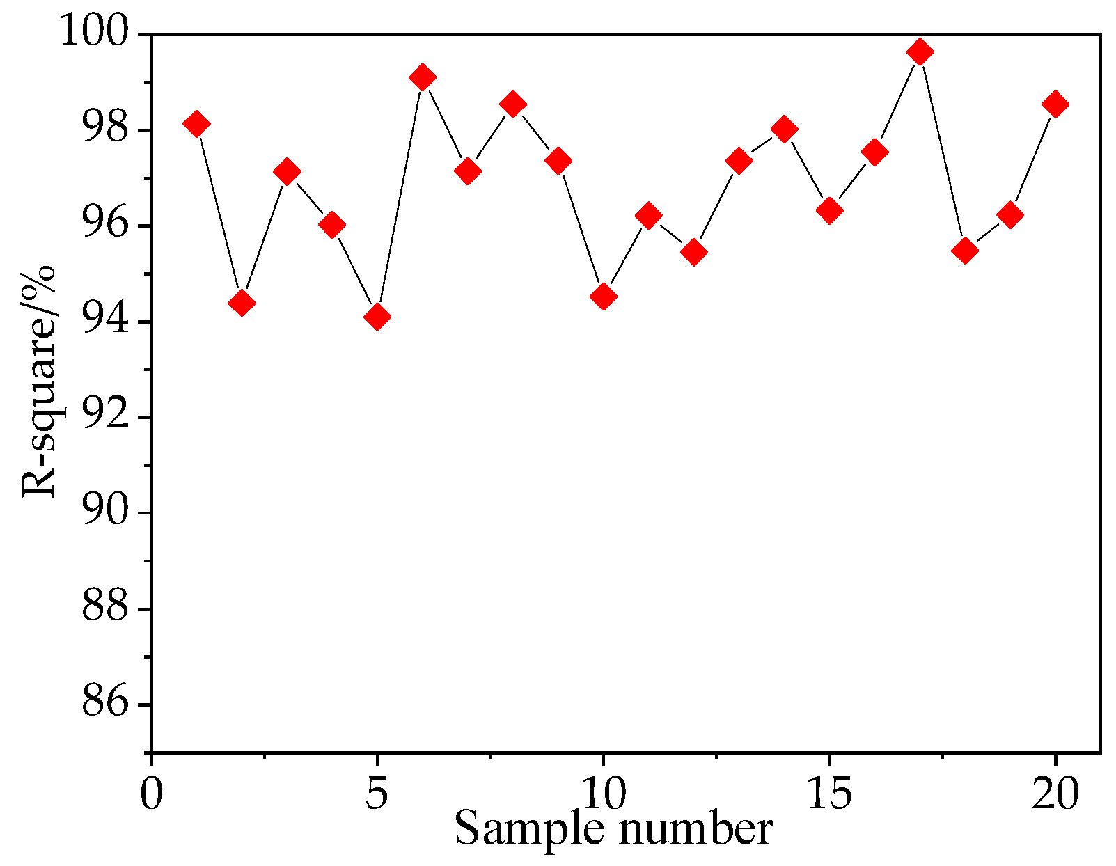
R-square is the coefficient of determination of the curve fit, which characterizes the quality of the quadratic polynomial fit, and the closer the value is to 1, the better the fit is. R-square is the curve fitting coefficient, which characterizes the quality of the quadratic polynomial fit, and the closer the value is to 1, the better the fit is. The fitting coefficients of the above four curves are all greater than 94%, which is a good fit. In addition, 20 groups of key point data were individually selected, their coefficients of determination in the least squares fitting were calculated, and R-square curves were plotted, as shown in Figure 8. The average R-square values of the fitted curves were all greater than 94%, indicating that the method can be used to fit the weld profile.
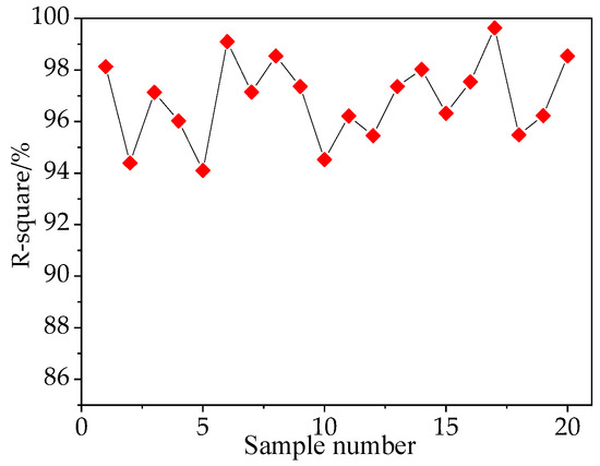
Figure 8.
Comparison of decision coefficients R-square.
3.3. Parameter Measurement Point Positioning
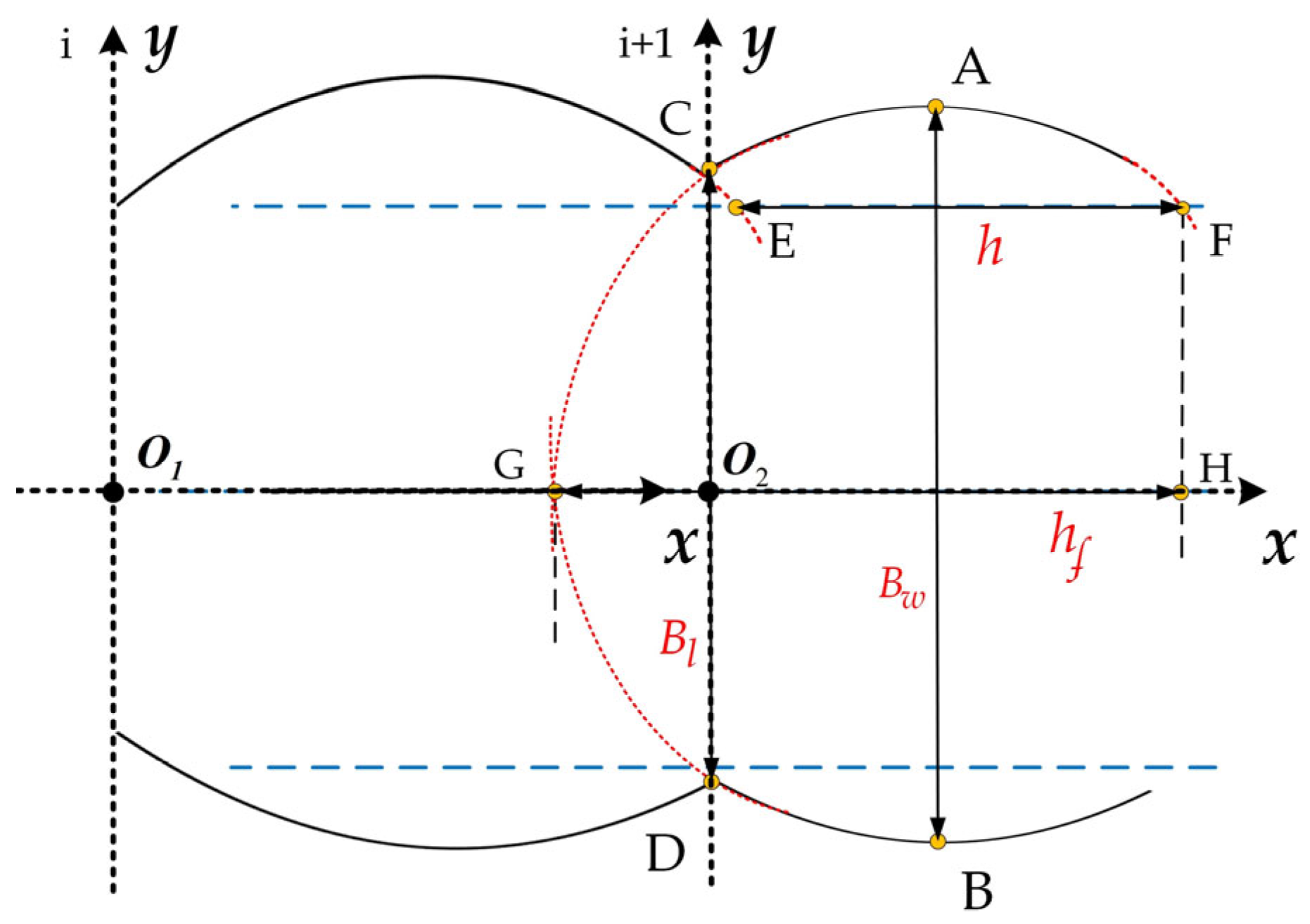
After the above series of processing of the “Measurement unit” image in Figure 3b, four fitted curves are obtained and placed in the weld coordinate system. To facilitate the derivation of the coordinates of the key measurement points, they are rotated clockwise, and the positions of the relevant measurement points are marked, as shown in Figure 9. The problem of solving the coordinates of all key measurement points can be transformed into the problem of finding special points by analytic functions. The location of the x-axis is the centerline of the weld, the blue dashed line symmetrical about the x-axis is the weld groove width line, and the line segment HF and the line segment length are known quantities.

Figure 9.
Coordinate positioning diagram of key measurement points.
Point A and point B are the extreme value of the fusion line, and their coordinates can be obtained by calculating the extreme value of the analytic function. The maximum sidewall fusion width is the sum of the absolute value of the vertical coordinates of points A and B. Point C and point D are the intersection of the fusion line and the y-axis, so that x = 0 to find its coordinates, and the bottom sidewall fusion width is the sum of the absolute value of the vertical coordinates of points C and D. Point E and point F are the intersection of the extension line of the x-axis direction of the adjacent fusion line and the weld groove width diagram line, respectively. Setting y = HF, the coordinates of the two points in the first quadrant of their respective coordinate systems can be obtained. The weld height is the horizontal coordinate of point F plus the length of the line segment minus the horizontal coordinate of point E. G point is the median point of the intersection of a pair of fusion line extension lines and the weld center line. Let the value of the corresponding analytic expression be 0, respectively, then the x-coordinate of G point is the mean value of the two x values obtained by solving. Point H is the projection point of point F on the x-axis, and its x-coordinate is known. The fusion depth is the sum of the absolute values of the abscess coordinates of two points. Because of the iterative relationship between adjacent passes, the height of weld is measured in the next “measurement unit”.
3.4. Measurement System Camera Calibration
In this paper, the coplanar linear calibration method is used to solve the hidden parameter matrix of the transformation from the world coordinate system to the image coordinate system; the schematic diagram is shown in step A of Figure 4. The details can be seen in the literature [19]. If the pixel coordinates of the maximum sidewall fusion width feature point A and B are and , respectively, the calculation process of the maximum sidewall melting width is as follows:
- Establish the internal and external parameter model of the camera.
Equation (1) is the in-camera parameter model, which is used to describe the conversion relationship between the image coordinate and the camera coordinate . Where , , is the focal length, is the camera main point coordinates, are the physical dimensions of the two coordinate axis directions in the image plane.
Equation (2) is an off-camera parameter model, which describes the conversion relationship between camera coordinates and world coordinates , where and are the rotation matrix and translation matrix in the world coordinate system relative to the camera coordinate system.
- Let the calibration plate and weld specimen be coplanar, the world coordinate system is established on the calibration plate; at this time , so the Formula (2) will be simplified by substituting into Formula (1) to obtain, this time:
, so eliminating and dividing by , we obtain
- The Harris corner point extraction method [20] was used to obtain the calibration plate corner points with known world and pixel coordinates, which were used to calculate the hidden parameter matrix .
- From Equations (3) and (4), the transformation relationship between the feature point image coordinate system and the world coordinate system can be obtained as
- The world coordinates of the feature point are
- Substituting the pixel coordinates of the points A and B into Equation (7), we obtain their world coordinates as
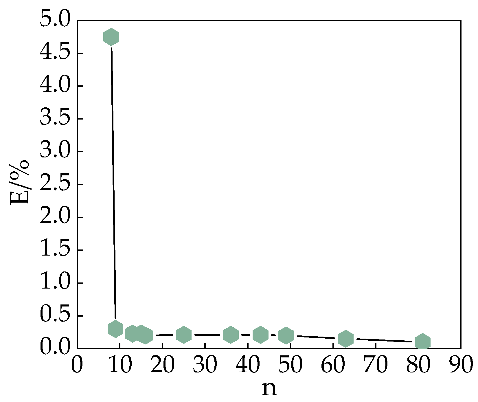
To verify the performance of the method, the influence of the number of corner points of the calibration plate on the measurement results was investigated. The results are shown in Figure 10. Under the premise that the number of corner points is greater than 10, the calibration algorithm is more stable, and the accuracy is higher, with a relative error of 0.013%.

Figure 10.
The influence of the number of corner points on the performance of the calibration plate.
4. Experimental Results and Analysis
4.1. Key Point Detection Experiment
4.1.1. Training Strategy and Evaluation Index
The Pytorch-1.7.1 deep learning framework was used; the operating system was Windows 10, the GPU was NVIDIA GTX 3090, and the processor was a 12th Intel(R) Core (TM) i9-12900KF CPU @2.40 GHz to train and test the HRnet network, and the training process used pre-trained models. The size of the dataset image is 256 × 192, the batch size is 8, and the epoch is 150. The initial learning rate (learning rate) is 0.01 using Adam optimization. The experiment used Average Precision (mAP) and Average Recall (AR) scores based on OKS (Object Key point Similarity, OKS) [21] as evaluation metrics.
4.1.2. Experimental Results
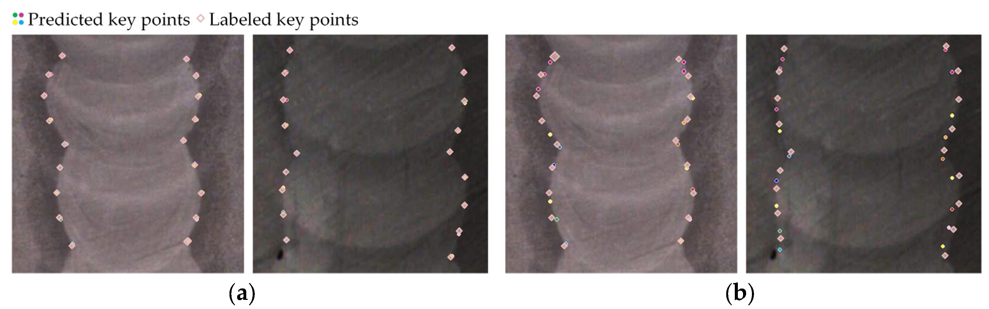
Using the above training strategy, the HRnet key point detection model was trained using the “measurement unit” key point dataset. The results are shown in Table 4, with an accuracy of 95.6% and a recall rate of 96.7%. The visualization results are shown in Figure 11. Figure 11a shows the detection results of the model trained for 150 epochs, and Figure 11b shows the detection results of the model trained for 50 epochs, where the colored circles are the predicted key points, and the diamonds are the labeled key points. It can be seen that the detection results of the model with 50 epochs of training are poor, and the key points are located with large deviations; the model with 150 epochs of training can accurately locate the key points. The training results and visualization results show that the model can achieve the accurate localization of key points.
Table 4.
HRnet network key point detection results.
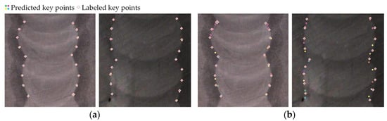
Figure 11.
Key point detection visualization results: (a) the detection results of the model trained for 150 epochs; (b) the detection results of the model trained for 50 epochs.
4.2. Feature Size Measurement Experiment
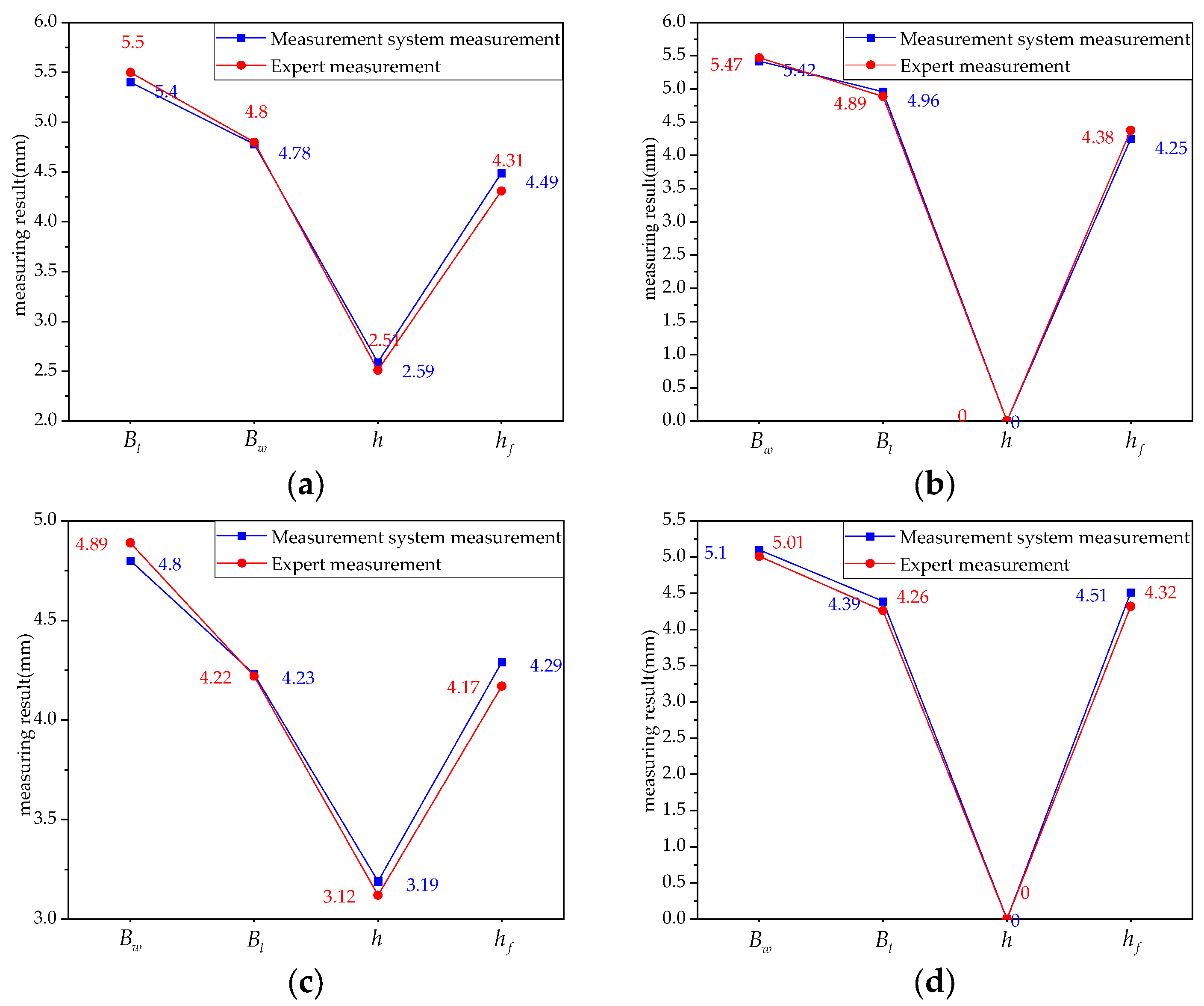
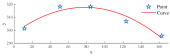
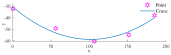
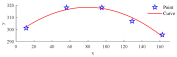
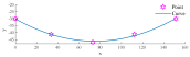
Two actual “measurement unit” with weld groove widths of 4.80 mm and 4.60 mm were selected, containing four weld seams (a), (b), (c), and (d), The four key dimensions , , , and were measured using both manual measurements by highly experienced experts and measurements by the measurement system, with the expert measurement distance defined as , the measurement system measurement distance defined as , the absolute error mean defined as , and the relative error means defined as . The obtained measurement results are shown in Figure 12 and Table 5.
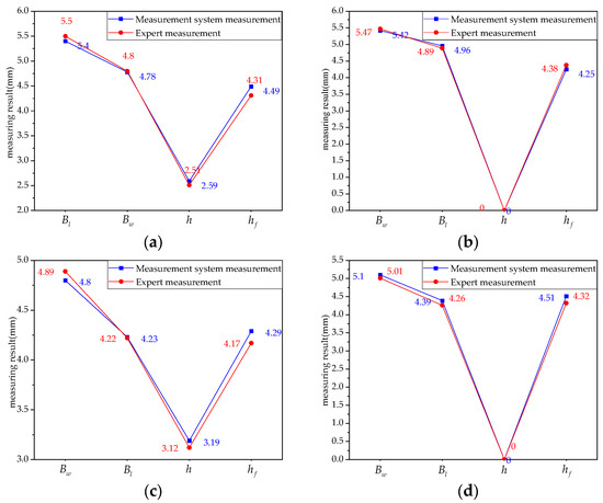
Figure 12.
Line graph display of measurement results: (a) results of the weld, (b) results of the weld, (c) results of the weld, (d) results of the weld. Note: The weld height of (b) weld and (d) weld is replaced by 0.
Table 5.
Measurement results of the two methods.
As can be seen from Table 4, the average absolute error in the measurement of the maximum sidewall fusion width is 0.08 mm, and the average relative error is 1.77%; the average absolute error in the measurement of the bottom sidewall fusion width is 0.06 mm and the average relative error is 1.27%; the average absolute error in the measurement of the weld height is 0.10 mm and the average relative error is 2.65%; the average absolute error in the measurement of the weld fusion depth is 0.15 mm and the average relative error was 3.12%. The results show that the absolute error of measurement is between 0.06 and 0.15 mm, the relative error is between 1.27% and 3.12%, the error is in the acceptable range, and the accuracy of the visual measurement system meets the requirements. The measurement efficiency was improved by one order of magnitude.
5. Conclusions
This paper presents a visual inspection method for weld profile fitting and geometric dimensioning based on a key point detection algorithm, which can be applied to single-layer multi-pass welding.
The weld profile is blurred, the difference is large, and the feature points are difficult to extract; so, the key point detection model is established, and the 18 key points of the “measurement unit” are automatically extracted, and the extraction accuracy reaches 95.6%.
The geometric model of the weld profile is obtained by fitting the characteristic points by least squares, and the fitted coefficients of determination, R-square, are all greater than 94%, and the measurement parameters are derived from the geometric relationships. The absolute errors of the measurements were between 0.06 and 0.15 mm, and the relative errors were between 1.27% and 3.12%, which improved the measurement rate by order of magnitude.
The camera is calibrated using a coplanar linear camera calibration algorithm to obtain the real distance corresponding to the actual pixel distance with a relative error of 0.013% in calibration.
Author Contributions
Conceptualization, W.H. and A.Z.; methodology, W.H., A.Z. and P.W.; software, W.H.; validation, W.H., A.Z. and P.W.; formal analysis, W.H.; investigation, W.H.; resources, A.Z. and P.W.; data curation, A.Z. and P.W.; writing—original draft preparation, W.H.; writing—review and editing, A.Z. and P.W.; supervision, A.Z.; funding acquisition, A.Z. and P.W. All authors have read and agreed to the published version of the manuscript.
Funding
This work was funded by the National Natural Science Foundation of China (62173170, 62001198), Gansu Province Science Foundation for Youths (20JR10RA186), State Key Laboratory of Synthetical Automation for Process Industries (2021-KF-21-04, 2020-KF-21-04), Key Laboratory of Gansu Advanced Control for Industrial Processes (2022KX02).
Institutional Review Board Statement
Not applicable.
Informed Consent Statement
Not applicable.
Data Availability Statement
Not applicable.
Conflicts of Interest
The authors declare no conflict of interest.
References
- Zhu, L.; Zhang, X.L.; Zheng, S.X.; Chen, J.H. Realization of ultra narrow gap welding with flux strips constraining arc. J. Lanzhou Univ. Technol. 2007, 3, 27–30. [Google Scholar]
- Zhang, X.L.; Zhu, L.; Huang, W.B.; Chen, J.H. Constricted Arc by Flux Strips Applied to Ultra-narrow Gap Welding. J. Mech. Eng. Chin. Ed. 2009, 45, 219–223. [Google Scholar] [CrossRef]
- Nagesh, D.S.; Datta, G.L. Genetic algorithm for optimization of welding variables for height to width ratio and application of ANN for prediction of bead geometry for TIG welding process. Appl. Soft Comput. 2010, 10, 897–907. [Google Scholar] [CrossRef]
- Mvola, B.; Kah, P.; Layus, P. Review of current waveform control effects on weld geometry in gas metal arc welding process. Int. J. Adv. Manuf. Technol. 2018, 96, 4243–4265. [Google Scholar] [CrossRef]
- Yang, Y.; Cao, L.C.; Zhou, Q.; Wang, C.C.; Wu, Q.; Jiang, P. Multi-objective process parameters optimization of Laser-magnetic hybrid welding combining Kriging and NSGA-II. Robot Comput. Integr. Manuf. 2018, 49, 253–262. [Google Scholar] [CrossRef]
- Sun, Q.J.; Cheng, W.Q.; Liu, Y.B. Research on rotating arc GMAW welding process characteristics. Trans. China Weld. Inst. 2015, 36, 29–32+114. [Google Scholar]
- Chang, Y.S.; Yue, J.F.; Guo, R.; Liu, W.J.; Li, L.Y. Penetration quality prediction of asymmetrical fillet root welding based on optimized BP neural network. J. Manuf. Process. 2020, 50, 247–254. [Google Scholar] [CrossRef]
- Chen, H.B.; Chen, S.B. Key Information Perception and Control Strategy of Intelligent Welding under Complex Scene. Acta Metall. Sin. 2022, 58, 541–550. [Google Scholar]
- Sun, J.H.; Zhang, C.Y.; Wu, J.Z.; Zhang, S.K. Prediction of weld profile of 31 6L stainless steel based on generalized regression neural network. Trans. China Weld. Inst. 2021, 42, 40–47+99. [Google Scholar]
- Zou, Y.Y.; Zuo, K.Z.; Li, P.F.; Cai, S. Geometric Modeling Methods for Cross-sectional Profile of Welds in Tailored Blank Laser Welding. Laser Optoelectron P. 2017, 54, 228–233. [Google Scholar]
- Wang, H.Y.; Zhang, Z.X.; Liu, L.M. Prediction and fitting of weld morphology of Al alloy-CFRP welding-rivet hybrid bonding joint based on GA-BP neural network. J. Manuf. Process. 2021, 63, 109–120. [Google Scholar] [CrossRef]
- Gao, Z.M.; Shao, X.Y.; Jiang, P.; Cao, L.C.; Zhou, Q.; Chen, Y.; Yang, L.; Wang, C.M. Parameters optimization of hybrid fiber laser-arc butt welding on 316L stainless steel using Kriging model and GA. Opt. Laser Technol. 2016, 83, 153–162. [Google Scholar] [CrossRef]
- Yu, J.; Cai, C.; Xie, J.; Liang, Y.; Huang, J.; Liu, Z.J.; Liu, Y.H. Process Parameter Optimization for Laser-Arc Hybrid Welding of Low-Carbon Bainite Steel Based on Response Surface Methodology. Chin. J. Lasers 2022, 49, 179–188. [Google Scholar]
- Wang, M.J.; Liu, X.Y.; Ma, X.X.; Chang, T.G.; Song, Q.F. Skeleton extraction method of single tillers rice based on stacked hourglass network. Trans. Chin. Soc. Agric. Eng. 2021, 37, 149–157. [Google Scholar]
- Bai, T.; Liu, S.; Wang, Y.; Wang, Y.; Dong, D. Self-Ensembling Semi-Supervised Model for Bone X-ray Images Landmark Detection. In Proceedings of the 2021 IEEE International Conference on Bioinformatics and Biomedicine (BIBM), Houston, TX, USA, 9–12 December 2021; pp. 817–822. [Google Scholar]
- Zhang, Y.; Wen, G.Z.; Mi, S.Y.; Zhang, M.L.; Geng, X. Overview on 2D Human Pose Estimation Based on Deep Learning. J. Softw. 2022, 33, 4173–4191. [Google Scholar]
- Sun, K.; Xiao, B.; Liu, D.; Wang, J. Deep High-Resolution Representation Learning for Human Pose Estimation. In Proceedings of the 2019 IEEE/CVF Conference on Computer Vision and Pattern Recognition (CVPR), Long Beach, CA, USA, 15–20 June 2019; pp. 5686–5696. [Google Scholar]
- Cheng, B.; Xiao, B.; Wang, J.; Shi, H.; Huang, T.S.; Zhang, L. Higher HRNet: Scale-Aware Representation Learning for Bottom-Up Human Pose Estimation. In Proceedings of the 2020 IEEE/CVF Conference on Computer Vision and Pattern Recognition (CVPR), Seattle, WA, USA, 13–19 June 2020; pp. 5385–5394. [Google Scholar]
- Yin, Y.J.; Xu, D.; Zhang, Z.T. Plane measurement based on monocular vision. J. Electron. Meas. Instrum. 2013, 27, 347–352. [Google Scholar] [CrossRef]
- Harris, C.; Stephens, M. A combined corner and edge detector. Alvey Vis. Conf. 1988, 15, 147–151. [Google Scholar]
- Lin, T.Y.; Michael, M.; Serge, B. Microsoft COCO: Common objects in context. In Proceedings of the 2014 European Conference on Computer Vision, Zurich, Switzerland, 6–12 September 2014; Springer: Cham, Switzerland, 2014; pp. 740–755. [Google Scholar]

Disclaimer/Publisher’s Note: The statements, opinions and data contained in all publications are solely those of the individual author(s) and contributor(s) and not of MDPI and/or the editor(s). MDPI and/or the editor(s) disclaim responsibility for any injury to people or property resulting from any ideas, methods, instructions or products referred to in the content. |
© 2023 by the authors. Licensee MDPI, Basel, Switzerland. This article is an open access article distributed under the terms and conditions of the Creative Commons Attribution (CC BY) license (https://creativecommons.org/licenses/by/4.0/).