Abstract
The supply of energy with the correct parameters to electrical appliances is possible with the use of energy converters. When a direct current is required, rectifier bridges are needed. These can be made using rectifier diodes. The problem of excessive junction temperatures in power diodes, which are used to build rectifier bridges and power converters, was recognized. For this reason, research work was carried out to create a model of a rectifier diode placed on a heat sink and to analyze the heat dissipation from the junction of this diode under forced convection conditions. The results obtained from the simulation work were compared with the results of thermographic temperature measurements. The boundary conditions chosen for the simulation work are presented. A method is also presented that determined the convection coefficient under forced convection conditions. The difference between the simulation results and the results of the thermographic measurements was found to be 0.1 °C, depending on the power dissipated at the junction and the air velocity around the diode.
1. Introduction
Power converters are used in renewable energy sources [1,2], in the electric vehicle industry [3,4], and wherever electricity must be supplied along with voltage adjustment to meet the needs of the device [5]. When a device requires a direct current, rectifier bridges are used [6]. One solution to provide a DC current to a device is to bridge four power diodes. Examples of such diodes are D61-200-22-N0-ABG [7], SCDR0240N12M [8], and D00-250-10 [9]. Diodes of this type can be used, for example, in the construction of a rectifier bridge used in electrical traction [10]. In [11,12], the problem associated with the excessive junction temperature of a semiconductor diode was pointed out.
The rise in temperature of a semiconductor diode is related to the power dissipated there [13]. The correct dissipation of heat from a semiconductor diode increases its useful life and the trouble-free operation time of the device in which it is installed [14]. The verification of the selection of the heat sink is possible based on the correct measurement of the junction temperature of a semiconductor diode. When the junction temperature is low, it means that little power has been dissipated in the junction or that the cooling system has been selected correctly. In these situations, it is possible that the cooling system has been oversized, and too much cost has been incurred as a result. Keeping the junction temperature of a semiconductor diode low indicates good heat dissipation from the junction and enables a device in which the diode is placed to be miniaturized.
On the other hand, when the junction temperature of a semiconductor diode is too high, it means that a lot of power has been dissipated at the diode junction. This is a situation that may not be safe due to the possibility of damage to the semiconductor diode. It also means that the wrong cooling system has been selected [15].
There are three ways to measure the junction temperature of a semiconductor diode:
- -
- Methods based on thermal sensitive parameter (TSP);
- -
- Methods which use contact sensors;
- -
- Methods which use non-contact sensors.
Electrical methods (based on TSP) involve determining the junction temperature of a semiconductor diode from the relationship between the temperature of the diode Tj and the conduction voltage VF. This is a method that is difficult to use. The relationship Tj = f(VF) is specific to the junction in question [16]. In order to designated this relationship, it is necessary to put the diode in the measurement circuit (outside the device containing this diode) and determine the characteristics. Because of this, the use of this method is troublesome.
Contact methods (which use contact sensors) require the temperature sensor to be applied to the case. Several temperature sensors are commonly used. Among the simplest of these are the thermocouple [17], the thermistor [18], and the thermoresistor [19]. The use of a thermocouple requires a device to compensate for the cold junction. This device can be found on a multimeter [20]. The thermistor has nonlinear characteristics that make it difficult to make a measurement. The use of any contact temperature sensor has an important disadvantage: the thermal conductivity relationship between the sensor case and the diode case is unknown. In addition, this conductivity depends on the temperature of the diode case. The result of the measurement of the contact temperature also depends on the contact force of the sensor case to the diode case [21]. Another significant disadvantage is the risk of electrical shock.
These disadvantages can be avoided by using thermographic measurements. Such a measurement involves determining the temperature of a diode case by analyzing the optical radiation reaching the radiation detectors in the thermal imaging camera. The thermal imaging measurement is not free of disadvantages. Its value depends on the emissivity factor value [22], the reflected temperature [23], the distance between the camera lens and the object under observation [24], the ambient temperature [25], the temperature of the external optical system [26], the transmission of the external optical system [27], and the relative humidity [28]. In addition, the result of a thermographic temperature measurement depends on the fuzziness of the recorded thermogram [29] and the location of the observation.
The thermographic measurement of the temperature of the diode case does not allow for the direct measurement of the semiconductor junction temperature. A measurement on the surface of the case is possible. The difference between the temperature of the semiconductor junction and the case temperature is due, among other things, to the thermal conductivity of the individual layers inside the case [30].
In the literature, many methods were described that can determine the difference between both the value of temperature of the diode case and the junction of a semiconductor diode. One of these methods designates the difference in temperature between the case temperature and the junction temperature based on a one-dimensional (1D) heat flow model. When a heat flow in a single component layer is analyzed, it is possible to compare the analyzed heat flux path to the one branch of the electrical circuit. The comparison is as follows: the electric potential can be compared to the temperature value of the one-sided analyzed layer, and the electrical resistance to the thermal resistance and the electric current flowing in the electrical branch can be compared to the heat flux in the analyzed path. For more layers in analyzed material, the thermal resistance of an individual material layer can be compared to the electrical resistance, which is connected in series in single branch [31]. When heat flow is analyzed for transient state, the thermal capacitance is also necessary to take into account. In this case, the model of heat flow shown as a series-connected resistance chain in one branch is replaced by a model shown as a chain of RC quadruples. In the literature, Foster’s [32] and Cauer’s [33] methods for the analysis of these RC quadruples were described. The Fourier equation was also used to determine the difference between the junction temperature of the diode and the temperature of the diode.
One-dimensional modeling does not allow the temperature distribution inside the semiconductor diode case to be determined. This is possible using the Finite Element Method. An additional advantage of using this method is the simple modeling of the effect of energy transfer via thermal radiation and by convection.
In the event that air flows around the diode under analysis at a speed greater than 0.5 m/s, forced convection must be taken into account. This is the case, for example, when the device containing the diode is in an open space. For this reason, it was decided to analyze the possibility of making an indirect thermal imaging measurement of a semiconductor diode on the basis of a thermogram and using an FEM. The diode was placed in a heat sink, and forced convection was taken into account.
Section 2.1 describes the diode used and the test rig constructed, while Section 2.2 describes the selection of boundary conditions for the simulation work carried out. Section 3 presents the results obtained. Section 4 comments on the results obtained. Section 5 presents the conclusions of the work carried out.
2. Materials and Methods
2.1. Measurement System and Equipment
In this work, a D00-250-10 power diode (Lamina, Piaseczno, Poland) (IF = 250 A, VF = 1.5 V) was used. The design of this diode is similar to that of the D61-200-22-N0-ABG diodes (Poweralia, Barcelona, Spain) and SCDR0240N12M diodes (Poweralia, Barcelona, Spain). The diode D00-250-10 is shown in Figure 1.
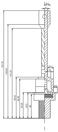
Figure 1.
D00-250-10 diode dimensions in millimeters.
The diode was placed in a heat sink. The dimensions of the heat sink and the placement of the diode are shown in Figure 2.
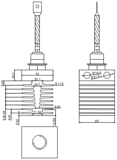
Figure 2.
Diode D00-250-10 mounted in a heat sink. Dimensions in millimeters.
The diode, together with the heat sink, was placed in a measurement system that allowed the measurement of the power dissipated in the diode. The value of the IF current that flowed through the observed diode was forced with the use of a CSU 600 A power source (Megger, Dover, England). The voltage drop across the terminals of the diode was measured using a UT55 voltmeter (UNI-T, Dongguan, China). In the work carried out, the temperature at the surface of the diode case was measured with an Optris Xi 400 thermal imaging camera (Optris, Berlin, Germany) with a telephoto lens (Instantaneous Field of View = 0.9 mrad). The accuracy of measurement was equal to 2 °C or 2%. The parameters of this thermographic camera were described in reference [34]. A schematic diagram of the part of the measurement system that allowed for forcing the current through the diode under test, measuring the power, and performing the measurement system is shown in Figure 3.
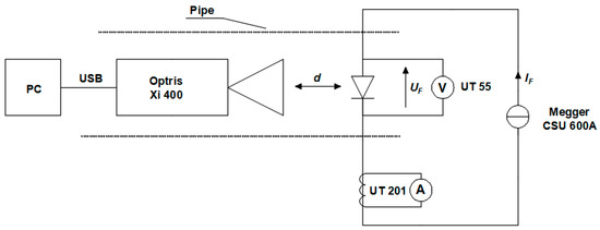
Figure 3.
Schematic diagram of a section of the measurement system that allowed the current to be forced through the diode under testing, the measurement of the power dissipated at the junction, and the thermal imaging of the diode case temperature.
To force the air flow around the observed diode, the diode, together with the heat sink, was placed in a tube. The tube was made of stainless steel, a material that has a low emissivity value ε. For this reason, the inside of the tube was lined with black polyurethane-made foam.
The structure of the foam used was porous. There is a similarity between the single pore foam and the black body model. Therefore, the walls of the chamber that was prepared were characterized by a high emissivity value of ε = 0.95 [35]. Additionally, the value of their reflectance p was low. For this reason, part of the measuring system, placed inside the chamber, was optically isolated.
The tube was mounted in a vertical orientation. A holder for a thermal imaging camera was placed inside the tube. Below this, a diode holder with a heat sink was placed. A fan was placed at the bottom of the resulting test rig to force air flow. The speed of the fan was controlled by a stepper motor controller, which in turn was controlled by a PLC (programmable logic controller) (Siemens S7-1200, 1215 DC/DC/DC). An HMI (Human Machine Interface) panel was attached to the PLC. A section of the measurement system that was responsible for the air flow around the diode under testing is shown in Figure 4.
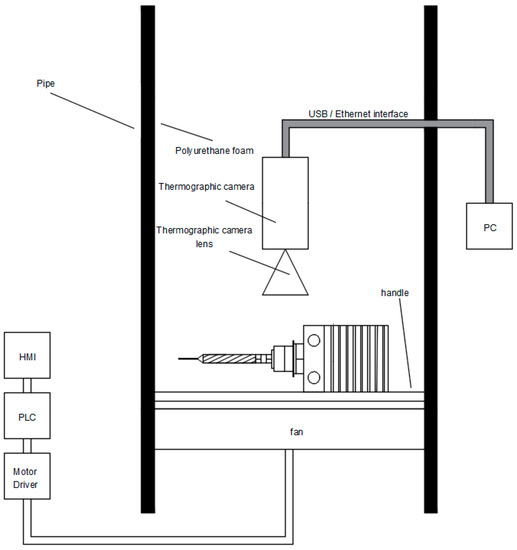
Figure 4.
Schematic diagram of a section of the measurement system that allowed air to be forced around the diode under testing. The diagram does not include the existing connection of the diode to the rest of the measurement system shown in Figure 3.
The air velocity in the tube was measured using GM 8903 (Benetech, Kalisz, Poland). By analyzing the system shown in Figure 4, it can be seen that the top of the tube was open. The heat sink and parts of the diode case were made of low-emissivity material. For this reason, markers were applied to the diode and the heat sink case using Velvet Coating 811-21 paint. The value of the emissivity coefficient of the paint used is known and is in the range of 0.970 to 0.975 when the temperature is between −36 °C and 82 °C. The uncertainty of the value of the emissivity coefficient is also known, and it is equal to 0.004 [36]. The arrangement of the markers placed on the diode case and their numbering are shown in Figure 5.
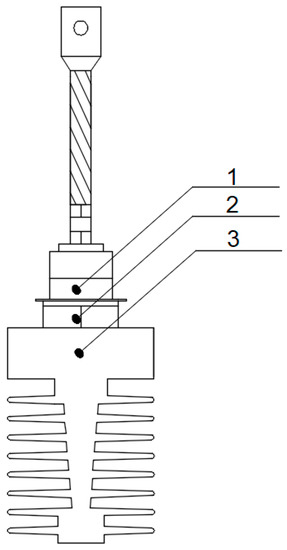
Figure 5.
Placement of markers made with Velvet Coating 811-21 paint and numbers given to each marker.
In order to eliminate the error associated with the observation angle, the observed diode surface was placed perpendicular to the lens of the thermal imaging camera.
2.2. Determining Convection Coefficients and Simulation Boundary Conditions
Determining the temperature distribution in a semiconductor diode case is possible after using the FEM method. This method consists of dividing the analyzed section of the case into a finite number of smaller solids of a specific shape. The nodes are located at the vertices of the resulting solids. Temperature information is stored at the node. The temperature values at certain nodes (e.g., those located on the section of the diode case that has been split) are set as a boundary condition. Knowing the heat flow equation that the software uses, the thermal properties (e.g., thermal resistance) of the material of the case fragment being analyzed, and the distances between nodes, the temperature distribution in the case can be determined.
The Solidworks 2020 SP05 software (Dassault Systèmes, Vélizy-Villacoublay, France) was used in the research carried out. The software allowed the necessary simulation work to be carried out through the use of FEM. The created model was subdivided into tetrahedral finite elements. The number of these elements can be specified by the user. Note that the more complex the model is, the more finite elements and nodes it will contain. Consequently, the greater the number of nodes (and finite elements), the more time is needed to calculate the values at the nodes and obtain the temperature distribution sought [37].
The equation that describes the transient heat conduction in a three-dimensional element can be written as follows (1) [38]:
where c is the specific heat; d is the density (kg/m3); kx, ky, and kz (W/(m·K)) are the thermal conductivities in the x, y, and z directions, respectively; T (K) is the temperature; and t (s) is the time.
In a steady state, when the heat flow in a single direction in a homogeneous environment is considered, Equation (2) can be used instead of Equation (1) [39]:
where J is a radiative heat flux (W∙m−2).
After separating the variables contained in Equation (2), the time constant can be obtained from the boundary conditions with Equation (3) [39]:
where xe is the end point of the analyzed heat flow path (m), T1 is the temperature at the starting point of the analyzed heat flow path (K), and T2 is the temperature at the end point of the analyzed heat flow path (K).
After separating the variables, integrating both sides and determining the time constant, Equation (2) takes the form of Equation (4) [39]:
where Pc is the total power, which was applied to the wall (W), and S is the area of the flat wall, which was penetrated by J.
Using Equation (4), the temperature difference between two points can be determined. In practice, the temperature distribution obtained in one line (1D model) might not provide enough data. For this reason, a 3D model is used to obtain more information. In each tetrahedral element (into which the semiconductor diode case is divided), the temperature field is interpolated based on the temperature at the nodes of that element and the linear shape function, Equation (5) [40]:
where Ti(t) is the nodal temperature at node i, and Hi is the linear shape function.
Determining the correct temperature distribution in the semiconductor diode case requires the determination of the radiation coefficient hr. In the Solidworks software used in the work carried out, the hr coefficient is determined from the value of ε. If the value of the hr coefficient is required, Equation (6) [41] can be used:
where σc is the Stefan–Boltzmann constant equal to 5.67 × 10⁻⁸ (W∙m−2∙K−4), TS is the surface temperature (K), and Ta is the air temperature (K).
In addition to the value of the hr coefficient, the value of the coefficient hc must be determined. This coefficient can be determined from Equation (7) [42]:
where hc is the convection coefficient of flat surfaces, Nu is the Nusselt number (-), and L is the characteristic length in meters (for a vertical wall, it is the height).
The Nusselt number for forced convection is described by Equation (8) [43]:
where Nu (-) is the Nuselt number, Pr (-) is the Prandtl number, Re (-) is the Reynolds number, and C, a, b are coefficients that depend on surface orientation (horizontal/vertical).
The values of C, a, and b coefficients are also dependent on the type of airflow. For flat horizontal surfaces, for laminar flow, Equation (8) takes the form of Equation (9) [44]:
Instead, for turbulent flow, Equation (8) takes the form of Equation (10) [44]:
The Prandtl number can be obtained using Equation (11) [45]:
where c is the specific heat of air equal to 1005 (J∙kg−1∙K−1) in 293.15 (K), and η is the dynamic air viscosity equal to 1.75 × 10⁻⁵ (kg∙m−1∙s−1) in 273.15 (K).
The Reynolds number can be obtained from Equation (12) [46]:
where V (m/s) is the average linear velocity of the fluid flow, and ρ is the air density equal to 1.21 (kg∙m−3) in 273.15 (K).
The roller surface value of the convection coefficient hcr can be obtained from Equation (13) [47]:
where d (m) is the dimension of the roller.
3. Results
In order to carry out reliable simulation work, the size of the mesh element was selected at the outset, and it was performed in such a way as to achieve convergence of results. The duration of the simulation was also recorded. The results obtained are presented in Table 1. As a representative point, an octagonal surface above the diode thread was selected.

Table 1.
The dependence of the convergence of the result and the simulation duration on the size of the mesh element.
Obtaining correct temperature distributions required the selection of correct values for the convection coefficients. This was conducted using Equations (7)–(13). The observed surface was oriented perpendicular to the direction of air flow. It was the rear surface of the solid that was hit by airflow. For this reason, the equations for turbulent flow were chosen. The selected materials, as well as the convection and thermal conductivity coefficients, are summarized in Table 2.
Table 2.
Assigned material and selected values for the convection coefficients hc/hcr (-) and the thermal conductivity coefficients k (W/(m·K)). The k-factor values were assigned to the selected materials by the software manufacturer.
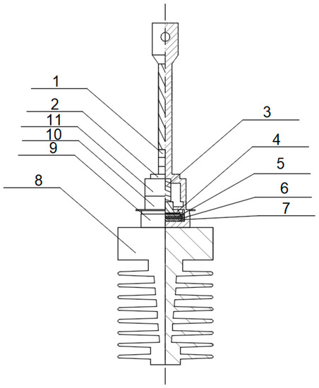
Figure 6.
Points with assigned properties, described in Table 2.
Using the test rig presented in Figure 4, thermograms were taken, as shown in Figure 7. Pj powers of 46.23 W, 74.48 W, and 111.75 W were dissipated at the diode junction. For each power, measurements were taken at air speeds of 0.75 m/s, 1 m/s, and 1.5 m/s. The thermograms are presented in Figure 7.
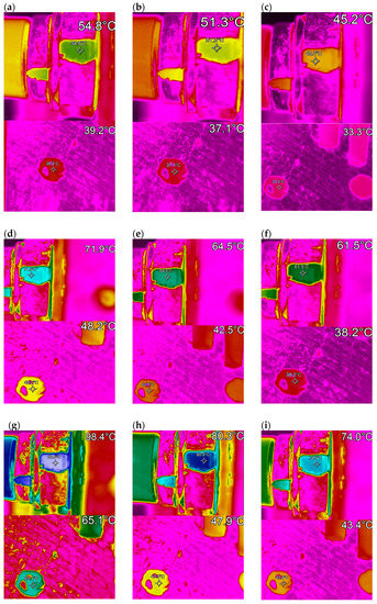
Figure 7.
Thermograms recorded for (a) Pj = 46.23 W and v = 0.75 m/s, (b) Pj = 46.23 W and v = 1 m/s, (c) Pj = 46.23 W and v = 1.5 m/s, (d) Pj = 74.48 W and v = 0.75 m/s, (e) Pj = 74.48 W and v = 1 m/s, (f) Pj = 74.48 W and v = 1.5 m/s, (g) Pj = 111.75 W and v = 0.75 m/s, (h) Pj = 111.75 W and v = 1 m/s, and (i) Pj = 111.75 W and v = 1.5 m/s.
The temperature distributions obtained from the simulation work are shown in Figure 8.
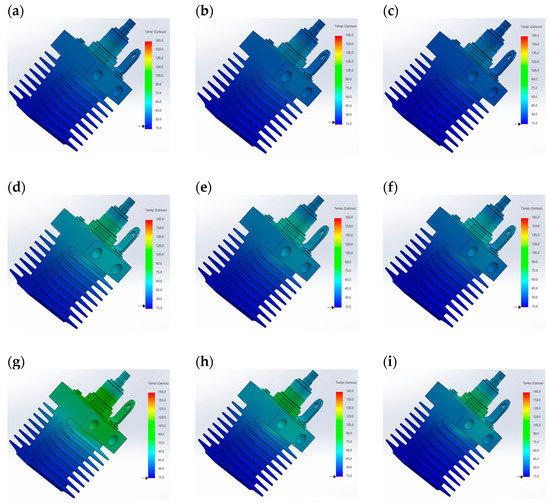
Figure 8.
Temperature distributions obtained for (a) Pj = 46.23 W and v = 0.75 m/s, (b) Pj = 46.23 W and v = 1 m/s, (c) Pj = 46.23 W and v = 1.5 m/s, (d) Pj = 74.48 W and v = 0.75 m/s, (e) Pj = 74.48 W and v = 1 m/s, (f) Pj = 74.48 W and v = 1.5 m/s, (g) Pj = 111.75 W and v = 0.75 m/s, (h) Pj = 111.75 W and v = 1 m/s, and (i) Pj = 111.75 W and v = 1.5 m/s.
The values of the convection coefficient for the cylinder hcr and the convection coefficient for the flat surface hcf for different values of Pj and v used in the simulation are presented in Table 3, Table 4 and Table 5.
Table 3.
The values of the convection coefficient for the cylinder hcr and the convection coefficient for the flat surface hcf used in the simulation for v = 0.75 m/s, v = 1 m/s, and v = 1.5 m/s; when the value of the power dissipated at the junction, Pj was 46.23 W (as marked in Figure 5).
Table 4.
The values of the convection coefficient for the cylinder hcr and the convection coefficient for the flat surface hcf used in the simulation for v = 0.75 m/s, v = 1 m/s, and v = 1.5 m/s; when the value of the power dissipated at the junction, Pj was 74.48 W (as marked in Figure 5).
Table 5.
The values of the convection coefficient for the cylinder hcr and the convection coefficient for the flat surface hcf used in the simulation for v = 0.75 m/s, v = 1 m/s, and v = 1.5 m/s; when the value of the power dissipated at the junction, Pj was 111.75 W (in marked in Figure 5).
A comparison of the results obtained from the TSym simulation and the results obtained from the TC measurements is shown in Table 6. The difference between Tc and Tj is shown in Table 6 and Table 7.
Table 6.
Comparison of the results obtained from the TSym simulations, and the results obtained from the TC measurements.
Table 7.
Comparison of the results obtained from the TC measurements and the junction temperatures Tj determined.
4. Discussion
The convergence of the measured temperatures of the diode case (the heat sink in which the diode is mounted) with the temperature obtained from the simulation work depends on the accuracy of the measurement and the accuracy of the simulation work. The accuracy of the results obtained from the simulation work depends, among other things, on the accuracy with which the values of the convection coefficients hcr and hcf were determined.
In the work carried out, the method of similarity to physical phenomena was used. This method makes it possible to obtain approximate values of the convection coefficients. In order to obtain more accurate values for the convection coefficients, they should be determined experimentally. The accuracy of the temperature distribution obtained from the simulation work also depends on the chosen size of the mesh element.
Figure 8 shows the heat dissipation with forced convection. Forced convection improves heat dissipation, and it can be seen that the diode case was colder. We can observe the heat dissipation on the diode case only.
The time shown in Table 1 is the simulation time for an illustrative size of the mesh element. Before starting the measurements, a preliminary study should be made to check the relationship between mesh element size, simulation time, and result accuracy. A mesh size should be chosen for which the simulation accuracy is satisfactory and the simulation time is not long. In the work carried out, the edge of the mesh element was 2.5 mm.
5. Conclusions
Energy converters make it possible to supply electricity with the appropriate parameters. When a direct current needs to be supplied, rectifier diodes are used in their design. Thermographic diagnostics of rectifier diodes make it possible to extend their service life, adjust the operating location to the design assumptions, verify the choice of heat sink, and even prevent failure. Consequently, it is possible to reduce operating costs.
The smallest difference between the temperature obtained from the simulation work and the experimental work was obtained at point 3–0.1 °C (Figure 5, Table 6). On the contrary, the smallest difference between the temperature of the case and the temperature of the junction was obtained at point 1–1.5 °C (Figure 5, Table 4).
On the basis of the experimental work carried out, the effectiveness of thermographic diagnostics under forced convection conditions can be confirmed. It was confirmed that, for air velocities not exceeding 1.5 m/s, it is possible to carry out an indirect thermographic measurement of the junction temperature of a semiconductor diode, i.e., a measurement whereby the junction temperature of the semiconductor can be determined from the measured temperature of the case. To perform this, it is necessary to monitor point 1 shown in Figure 5.
The value of the convection coefficient increases with increasing air velocity and decreases with increasing surface temperature. In the work carried out, the value of the convection coefficient ranged from approximately 21 to approximately 77. This value depends on the shape of the surface, on the orientation of the surface, and on the speed of the air that flows around the surface.
By analyzing the thermograms shown in Figure 7, it can be seen that, as the airflow velocity increases for the same Pj power values that were discharged at the junction, the recorded temperatures of the heat sink and the diode case are lower. This indicates an improvement in heat dissipation from these surfaces. This trend can be seen for all the power values of Pj that were discharged.
The temperature distributions that were determined from the simulation work (Figure 8) confirm the thermographic measurements. Consequently, it is possible to conclude that the recorded thermograms are reliable. It can also be concluded that, for air velocities of no more than 1.5 m/s, the thermographic measurement of the surface temperature of the power diode and the heat sink (on which it is placed) is reliable.
By analyzing the data in Table 6, it can be seen that the temperature obtained on the surface Tc differed from the joint temperature Tsym, which was determined from the simulation work. The smallest differences can be observed for point 2 (shown in Figure 5). The largest difference that was recorded for this point did not exceed 1.5 °C.
Author Contributions
Methodology, A.H. and K.D.; formal analysis, A.H. and K.D.; investigation A.H. and K.D.; resources K.D. and Ł.D; writing—original draft preparation, K.D., A.H. and Ł.D.; writing—review and editing, K.D., A.H., Ł.D. and G.D.; visualization A.H. and K.D.; supervision, A.H. and K.D. All authors have read and agreed to the published version of the manuscript.
Funding
This research was funded by the Ministry of Education and Science of Poland (grant numbers 0212/SBAD/0593, 0212/SBAD/0595 and 0711/SBAD/4616).
Institutional Review Board Statement
Not applicable.
Informed Consent Statement
Not applicable.
Data Availability Statement
Not applicable.
Conflicts of Interest
The authors declare no conflict of interest.
Nomenclatures
| Tj | junction temperature |
| VF | forward voltage |
| IF | forward current |
| λ | wavelength |
| ε | emissivity factor |
| p | reflectance factor |
| c | specific heat |
| d | density |
| kx, ky and kz | thermal conductivities in the directions x, y, and z directions |
| T | temperature |
| t | time |
| J | radiative heat flux |
| Pc | total power |
| S | the area of the flat wall, which was penetrated by J |
| i | node number |
| Hi | linear shape function |
| hr | radiation coefficient |
| σc | Stefan–Boltzmann constant |
| Ta | air temperature |
| TS | surface temperature |
| hc | convection coefficient of flat surfaces |
| Nu | Nusselt number |
| L | characteristic length |
| Pr | Prandtl number |
| Re | Reynolds number |
| C, a, b | coefficients depend on surface orientation (horizontal/vertical) |
| η | dynamic air viscosity |
| V | average linear velocity of fluid flow |
| hcr | convection coefficient for roller surface |
| d | dimension of roller |
| ρ | air density equal |
| k | thermal conductivity |
| TSym | results obtained simulation |
| TC | results obtained from thermographic measurement |
References
- Senturk, O.S.; Helle, L.; Munk-Nielsen, S.; Rodriguez, P.; Teodorescu, R. Converter structure-based power loss and static thermal modeling of the press-pack IGBT three-level ANPC VSC applied to multi-MW wind turbines. IEEE Trans. Ind. Appl. 2011, 47, 2505–2515. [Google Scholar] [CrossRef]
- Nakamura, Y. Electrothermal Cosimulation for Predicting the Power Loss and Temperature of SiC MOSFET Dies Assembled in a Power Module. IEEE Trans. Power Electron. 2020, 35, 2950–2958. [Google Scholar] [CrossRef]
- Amiri, P.; Eberle, D.; Gautam, D.; Botting, C.A. CCM Bridgeless Single-Stage Soft-Switching AC-DC Converter for EV Charging Application. In Proceedings of the 2021 IEEE Energy Conversion Congress and Exposition (ECCE), Vancouver, BC, Canada, 10–14 October 2021; pp. 1846–1852. [Google Scholar] [CrossRef]
- Ciappa, M.; Fichtner, W.; Kojima, T.; Yamada, Y.; Nishibe, Y. Extraction of accurate thermal compact models for fast electro-thermal simulation of IGBT modules in hybrid electric vehicles. Microelectron. Reliab. 2005, 45, 1694–1699. [Google Scholar] [CrossRef]
- Gorji, S.A.; Sahebi, H.G.; Ektesabi, M.; Rad, A.B. Topologies and control schemes of bidirectional DC–DC power converters: An overview. IEEE Access 2019, 7, 117997–118019. [Google Scholar] [CrossRef]
- Busatto, T.; Rönnberg, S.K.; Bollen, M.H.J. Comparison of Models of Single-Phase Diode Bridge Rectifiers for Their Use in Harmonic Studies with Many Devices. Energies 2022, 15, 66. [Google Scholar] [CrossRef]
- D61-200-22-NO-ABG. Available online: https://www.poweralia.com/d61-200-22-n0-abg-pw (accessed on 14 February 2023).
- SCDR0240N12M. Available online: https://www.poweralia.com/scdr0240n12m-pw (accessed on 14 February 2023).
- Dziarski, K.; Hulewicz, A.; Dombek, G.; Drużyński, Ł. Indirect Thermographic Temperature Measurement of a Power-Rectifying Diode Die. Energies 2022, 15, 3203. [Google Scholar] [CrossRef]
- Plesca, A.; Mihet-Popa, L. Thermal Analysis of Power Rectifiers in Steady-State Conditions. Energies 2020, 13, 1942. [Google Scholar] [CrossRef]
- Hayashi, Y.; Takao, K.; Adachi, K.; Ohashi, H. Design consideration for high output power density (OPD) converter based on power-loss limit analysis method. In Proceedings of the 2005 European Conference on Power Electronics and Applications, Dresden, Germany, 11–14 September 2005; IEEE: Piscataway, NJ, USA, 2005; pp. 1–9. [Google Scholar] [CrossRef]
- Li, X.; Li, D.; Qi, F.; Packwood, M.; Luo, H.; Liu, G.; Dai, X. Advanced Electro-Thermal Analysis of IGBT Modules in a Power Converter System. In Proceedings of the 2019 20th International Conference on Thermal, Mechanical and Multi-Physics, Hannover, Germany, 24–27 March 2019; IEEE: Piscataway, NJ, USA, 2019; pp. 1–4. [Google Scholar] [CrossRef]
- Kasprzak, M.; Sledzinska, M.; Zaleski, K.; Iatsunskyi, I.; Alzina, F.; Volz, S.; Torres, C.M.S.; Graczykowski, B. High-temperature silicon thermal diode and switch. Nano Energy 2020, 78, 105261. [Google Scholar] [CrossRef]
- Ostapchuk, M.; Shishov, D.; Shevtsov, D.; Zanegin, S. Research of Static and Dynamic Properties of Power Semiconductor Diodes at Low and Cryogenic Temperatures. Inventions 2022, 7, 96. [Google Scholar] [CrossRef]
- Teo, J.C.; Tan, R.H.G.; Mok, V.H.; Ramachandaramurthy, V.K.; Tan, C. Impact of bypass diode forward voltage on maximum power of a photovoltaic system under partial shading conditions. Energy 2020, 191, 116491. [Google Scholar] [CrossRef]
- Available online: https://www.jedec.org/ (accessed on 14 February 2023).
- Leonidas, E.; Ayvar-Soberanis, S.; Laalej, H.; Fitzpatrick, S.; Willmott, J.R. A Comparative Review of Thermocouple and Infrared Radiation Temperature Measurement Methods during the Machining of Metals. Sensors 2022, 22, 4693. [Google Scholar] [CrossRef]
- Shariq, M.; Asim Siddiqui, M.; Qamar, M.A.; Altowairqi, Y.; Ali, S.K.; Madkhali, O.; Fadhali, M.M.; Alharbi, T.; Khan, M.S.; Saheb Syed, I.; et al. Study of Co-Doped K2Ti6O13 Lead-Free Ceramic for Positive Temperature Coefficient Thermistor Applications. Crystals 2022, 12, 1569. [Google Scholar] [CrossRef]
- Zhang, H.; Teoh, J.C.; Wu, J.; Yu, L.; Lim, C.T. Dynamic Zero Current Method to Reduce Measurement Error in Low Value Resistive Sensor Array for Wearable Electronics. Sensors 2023, 23, 1406. [Google Scholar] [CrossRef] [PubMed]
- Wang, F.; Lin, Z.; Zhang, Z.; Li, Y.; Chen, H.; Liu, J.; Li, C. Fabrication and Calibration of Pt-Rh10/Pt Thin-Film Thermocouple. Micromachines 2023, 14, 4. [Google Scholar] [CrossRef] [PubMed]
- Zaccara, Z.; Edelman, J.B.; Cardone, G. A general procedure for infrared thermography heat transfer measurements in hypersonic wind tunnels. Int. J. Heat Mass Transf. 2020, 163, 120419–120435. [Google Scholar] [CrossRef]
- Altenburg, J.S.; Straße, A.; Gumenyuk, A.; Meierhofer, C. In-situ monitoring of a laser metal deposition (LMD) process: Comparison of MWIR, SWIR and high-speed NIR thermography. Quant. InfraRed Thermogr. J. 2020, 19, 97–114. [Google Scholar] [CrossRef]
- Yoon, S.T.; Park, J.C. An experimental study on the evaluation of temperature uniformity on the surface of a blackbody using infrared cameras. Quant. InfraRed Thermogr. J. 2021, 19, 172–186. [Google Scholar] [CrossRef]
- Schuss, C.; Remes, K.; Leppänen, K.; Saarela, J.; Fabritius, T.; Eichberger, B.; Rahkonen, T. Detecting Defects in Photovoltaic Cells and Panels with the Help of Time-Resolved Thermography under Outdoor Environmental Conditions. In Proceedings of the 2020 IEEE International Instrumentation and Measurement Technology Conference (I2MTC), Dubrovnik, Croatia, 25–28 May 2020; pp. 1–6. [Google Scholar] [CrossRef]
- Chakraborty, B.; Billol, K.S. Process-integrated steel ladle monitoring, based on infrared imaging—A robust approach to avoid ladle breakout. Quant. InfraRed Thermogr. J. 2020, 17, 169–191. [Google Scholar] [CrossRef]
- Tomoyuki, T. Coaxiality Evaluation of Coaxial Imaging System with Concentric Silicon–Glass Hybrid Lens for Thermal and Color Imaging. Sensors 2020, 20, 5753. [Google Scholar] [CrossRef]
- Wollack, J.E.; Cataldo, G.; Miller, K.H.; Quijada, A.M. Infrared properties of high-purity silicon. Opt. Lett. 2020, 45, 4935–4938. [Google Scholar] [CrossRef]
- Singh, J.; Arora, A.S. Effectiveness of active dynamic and passive thermography in the detection of maxillary sinusitis. Quant. InfraRed Thermogr. J. 2020, 18, 213–225. [Google Scholar] [CrossRef]
- Dziarski, K.; Hulewicz, A.; Dombek, G. Lack of Thermogram Sharpness as Component of Thermographic Temperature Measurement Uncertainty Budget. Sensors 2021, 21, 4013. [Google Scholar] [CrossRef]
- Dziarski, K.; Hulewicz, A.; Dombek, G. Thermographic Measurement of the Temperature of Reactive Power Compensation Capacitors. Energies 2021, 14, 5736. [Google Scholar] [CrossRef]
- Xu, J.; Wang, X.; Shi, H.; Mei, X. Multi-scale short circuit resistance estimation method for series connected battery strings. Energy 2020, 202, 117647. [Google Scholar] [CrossRef]
- Valdivieso, C.A.; Meunier, G.; Ramdane, B.; Gyselinck, J.; Guerin, C.; Sabariego, R.V. Time-Domain Finite-Element Eddy-Current Homogenization of Windings Using Foster Networks and Recursive Convolution. IEEE Trans. Magn. 2020, 56, 7401408. [Google Scholar] [CrossRef]
- Sato, Y.; Shimotani, T.; Igarashi, H. Synthesis of Cauer-Equivalent Circuit Based on Model Order Reduction Considering Nonlinear Magnetic Property. IEEE Trans. Magn. 2017, 53, 1100204. [Google Scholar] [CrossRef]
- Optris XI 400. Available online: https://www.optris.global/optris-xi-400?gclid=CjwKCAiAoL6eBhA3EiwAXDom5iDyJ7ANskvy59t3eZIY5ngbPO7LCh2NPJaQ94OcHAQARnbD_K9rxxoCSbkQAvD_BwE (accessed on 24 January 2023).
- Krawiec, P.; Rózański, L.; Czarnecka-Komorowska, D.; Warguła, Ł. Evaluation of the Thermal Stability and Surface Characteristics of Thermoplastic Polyurethane V-Belt. Materials 2020, 7, 1502. [Google Scholar] [CrossRef] [PubMed]
- Kawor, E.T.; Mattei, S. Emissivity measurements for nexel velvet coating 811-21 between −36 °C and 82 °C. High Temp. High Press. 1999, 33, 551–556. [Google Scholar] [CrossRef]
- Li, H. The Finite Element Method. In Graded Finite Element Methods for Elliptic Problems in Nonsmooth Domains; Surveys and Tutorials in the Applied Mathematical Sciences; Springer: Cham, Switzerland, 2022; Volume 10. [Google Scholar] [CrossRef]
- Feng, S.Z.; Cui, X.Y.; Li, G.Y. Transient thermal mechanical analyses using a face-based smoothed finite element method (FS-FEM). Int. J. Therm. Sci. 2013, 74, 95–103. [Google Scholar] [CrossRef]
- Devloo, P.R.B.; Bravo, C.M.A.A.; Rylo, E.C. Systematic and generic construction of shape functions for p-adaptive meshes of multidimensional finite elements. Comput. Methods Appl. Mech. Eng. 2009, 198, 1716–1725. [Google Scholar] [CrossRef]
- Dziarski, K.; Hulewicz, A.; Drużyński, Ł.; Dombek, G. Indirect Thermographic Temperature Measurement of a Power-Rectifying Diode Die Based on a Heat Sink Thermogram. Energies 2023, 16, 332. [Google Scholar] [CrossRef]
- Ghahfarokhi, P.S. Determination of Forced Convection Coefficient over a Flat Side of Coil. In Proceedings of the 2017 IEEE 58th International Scientific Conference on Power and Electrical Engineering of Riga Technical University (RTUCON), Riga, Latvia, 12–13 October 2017. [Google Scholar] [CrossRef]
- Aminu, Y.; Ballikaya, S. Thermal resistance analysis of trapezoidal concentrated photovoltaic–Thermoelectric systems. Energy Convers. Manag. 2021, 250, 114908. [Google Scholar] [CrossRef]
- Available online: https://repozytorium.biblos.pk.edu.pl/redo/resources/30992/file/suwFiles/DudaP_WyznaczanieWspolczynnika.pdf (accessed on 14 February 2023).
- Available online: https://www.sciencedirect.com/science/article/pii/S0038092X05003701 (accessed on 14 February 2023).
- Poppe, A.; Farkas, G.; Gaál, L.; Hantos, G.; Hegedüs, J.; Rencz, M. Multi-Domain Modelling of LEDs for Supporting Virtual Prototyping of Luminaires. Energies 2019, 12, 1909. [Google Scholar] [CrossRef]
- Available online: https://www.sciencedirect.com/science/article/pii/S0017931018362045 (accessed on 15 February 2023).
- Kosmol, J. Modeling of Heat Phenomenon in Rolling Kinematic Pairs Using the Finite Element Method. Appl. Sci. 2021, 11, 6447. [Google Scholar] [CrossRef]


Disclaimer/Publisher’s Note: The statements, opinions and data contained in all publications are solely those of the individual author(s) and contributor(s) and not of MDPI and/or the editor(s). MDPI and/or the editor(s) disclaim responsibility for any injury to people or property resulting from any ideas, methods, instructions or products referred to in the content. |
© 2023 by the authors. Licensee MDPI, Basel, Switzerland. This article is an open access article distributed under the terms and conditions of the Creative Commons Attribution (CC BY) license (https://creativecommons.org/licenses/by/4.0/).