

Buckle Pose Estimation Using a Generative Adversarial Network


Abstract
1. Introduction
- (1)
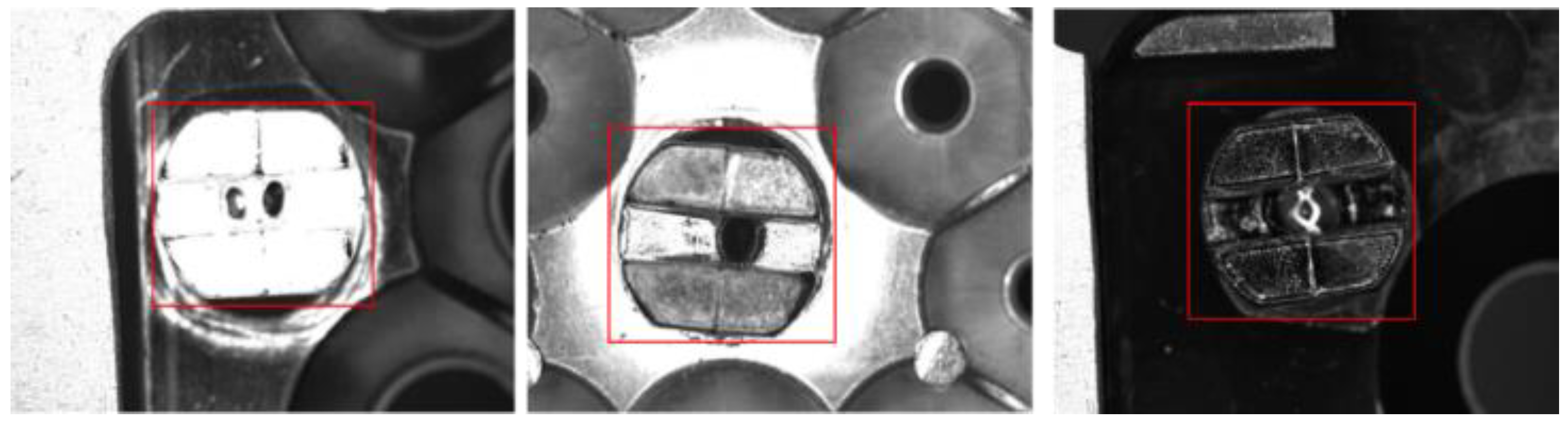
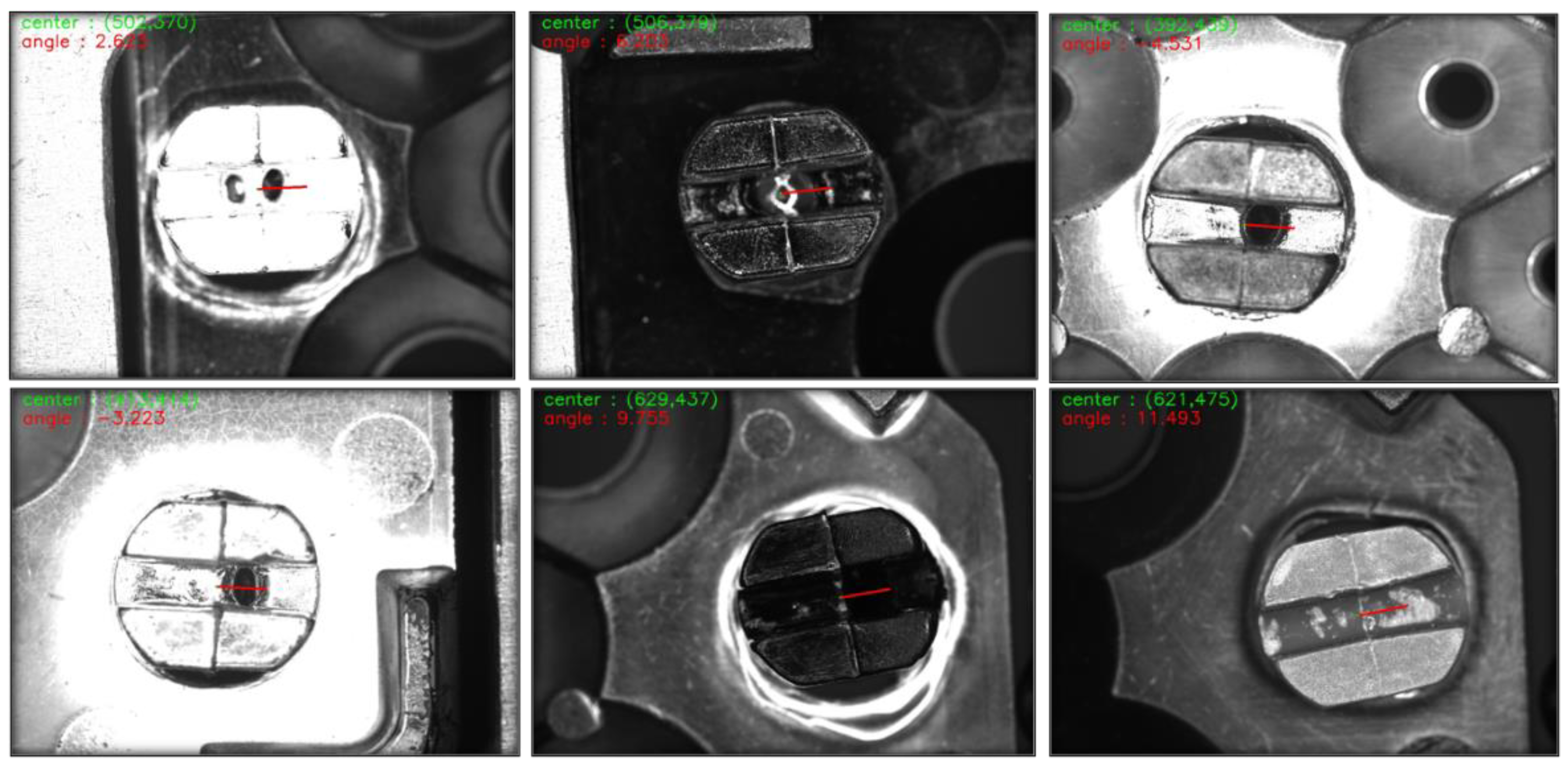
- The model must be generalizable enough to adaptively handle significant buckle shape differences. Figure 1 presents three common buckle types (buckles are inside the red box).
- (2)
- The model must distinguish the buckle from its background. The differences between these two are small. Figure 1 illustrate this scenario.
- (3)
- The accuracy of buckle pose estimation must be high enough to reduce the loss caused by the clumsy disassembly of the machine.
2. Related Work
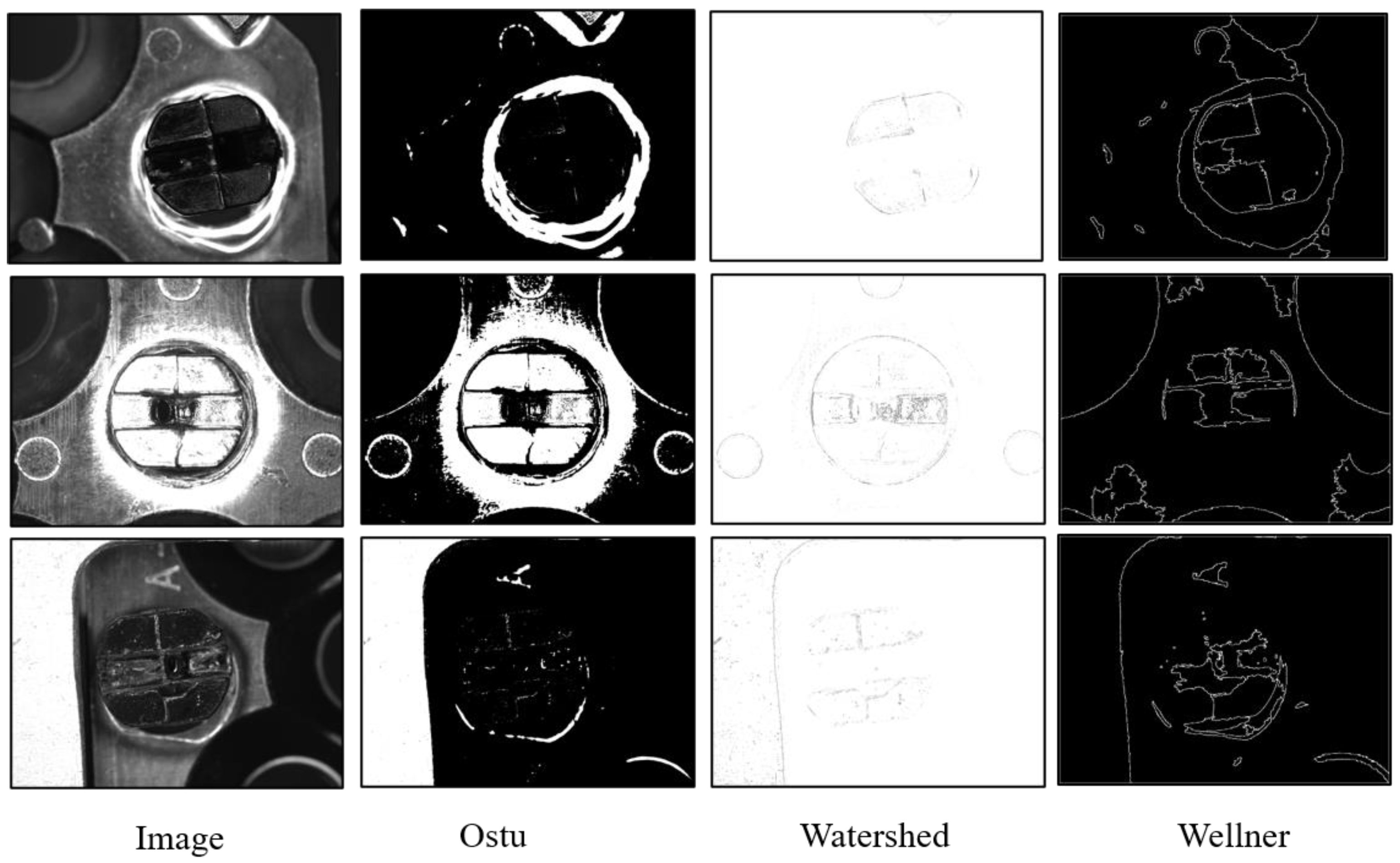
2.1. Traditional Detection Approaches
2.2. Deep Learning Detection Approaches
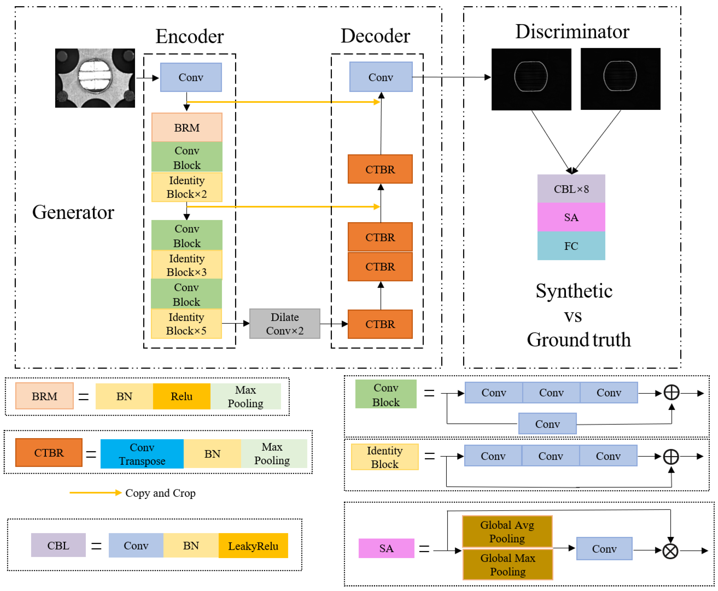
3. Methods
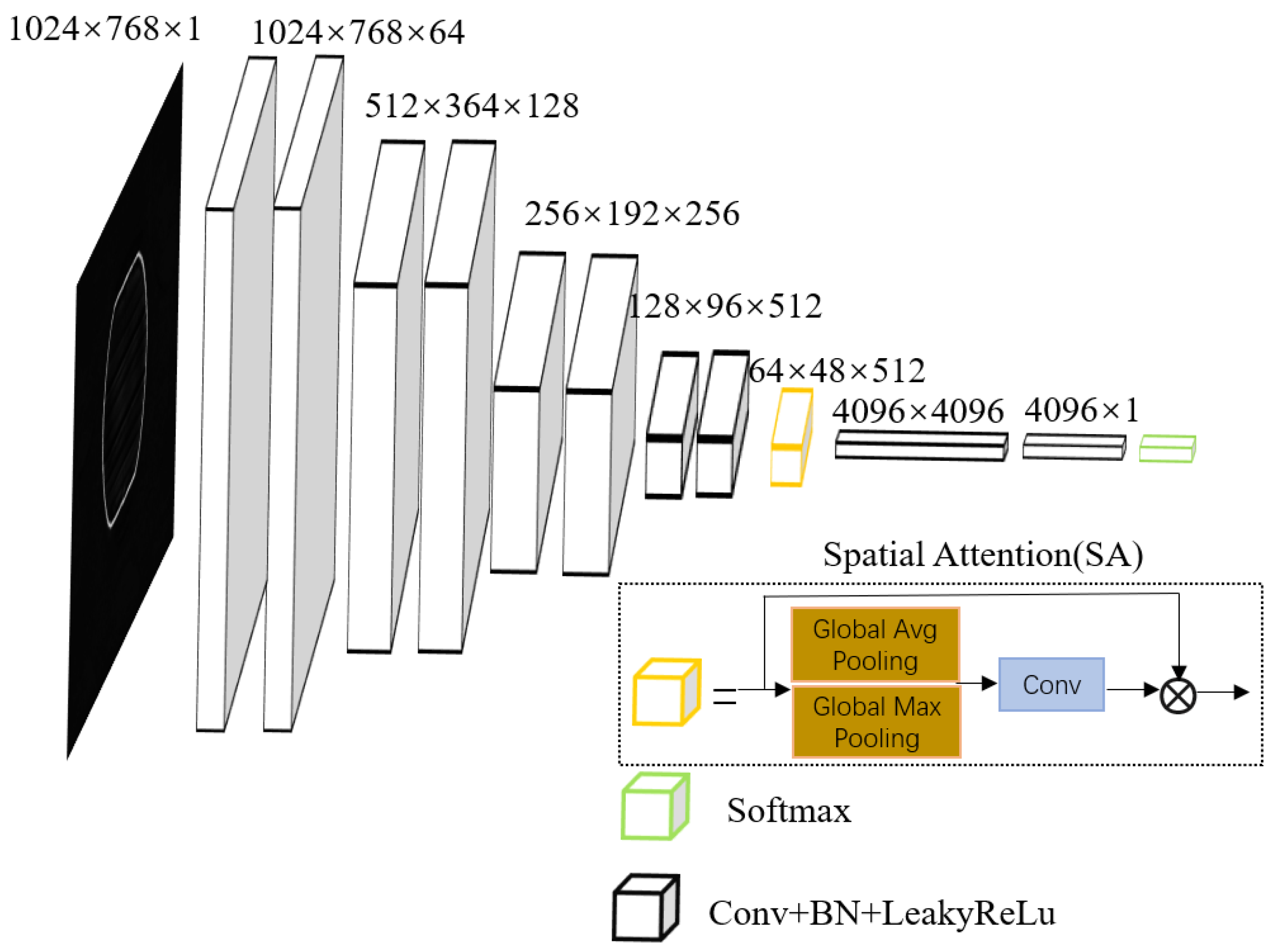
3.1. Feature Extraction Module
3.2. Feature Reconstruction Module
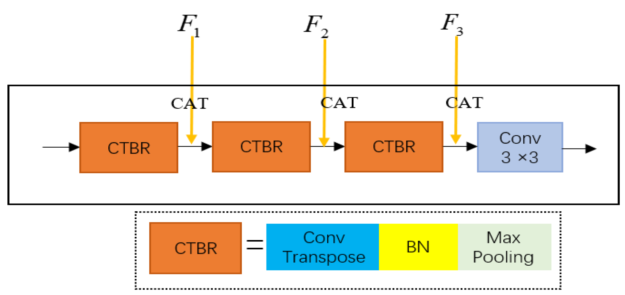
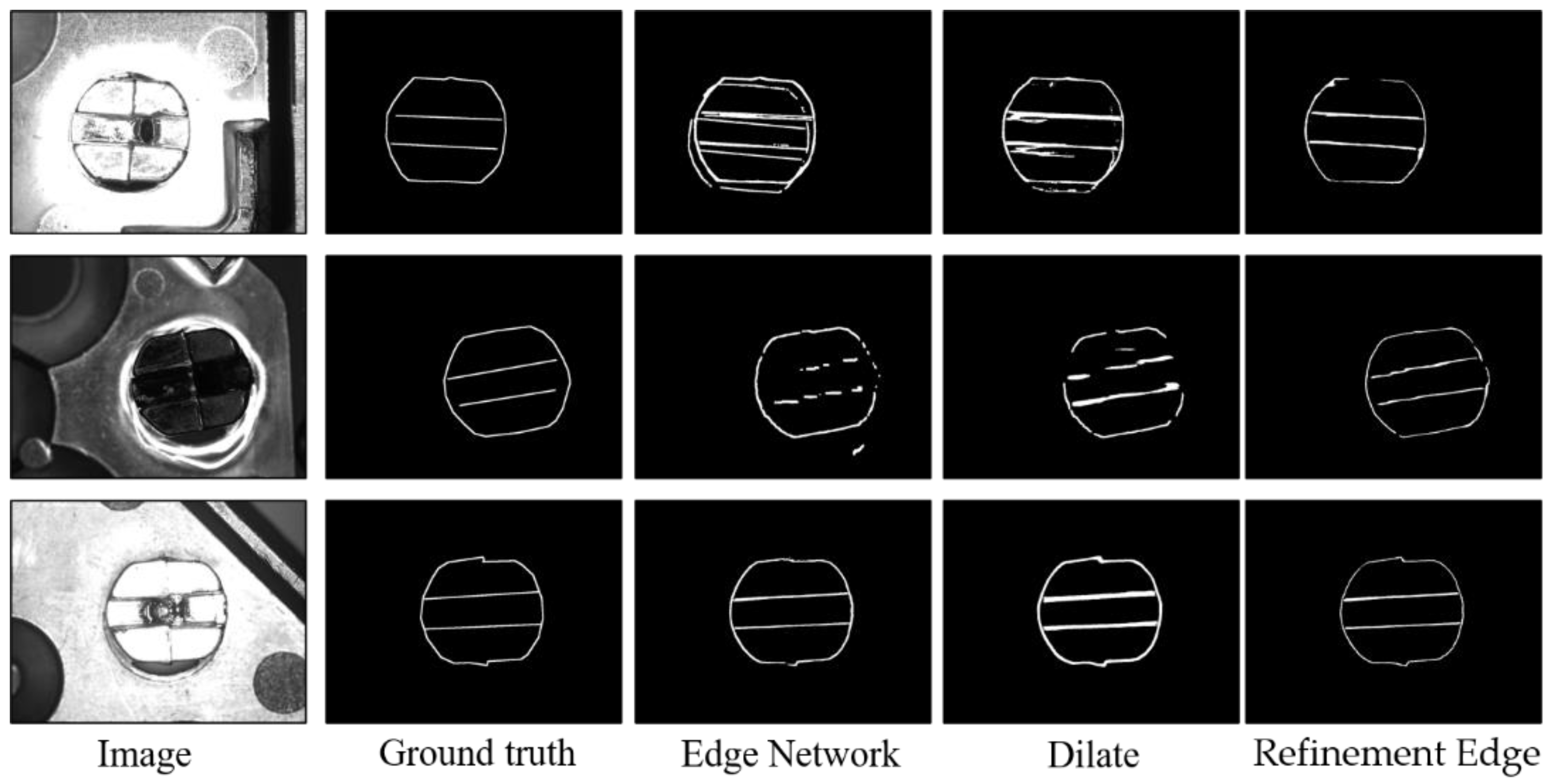
3.3. Refinement Edge Module
4. Experiments and Results
4.1. Datasets
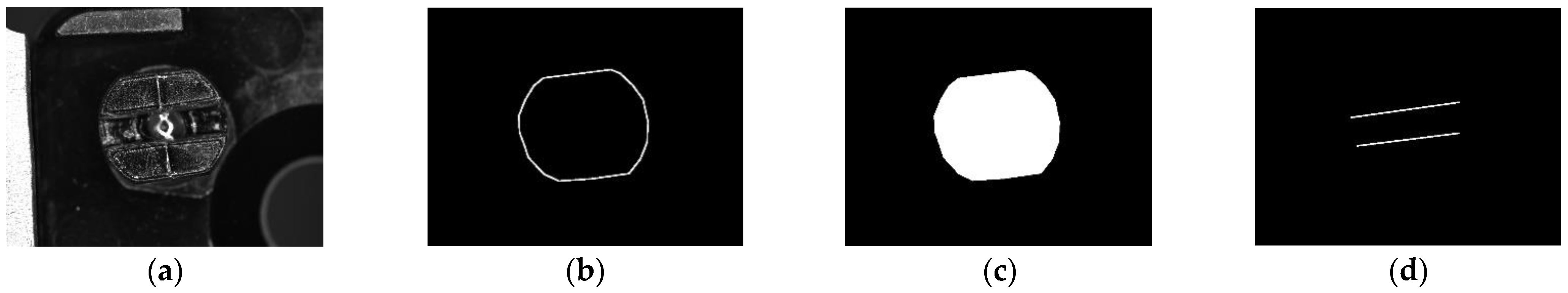
4.2. Training Label
4.3. Experimental Environment
4.4. Evaluation Methodology
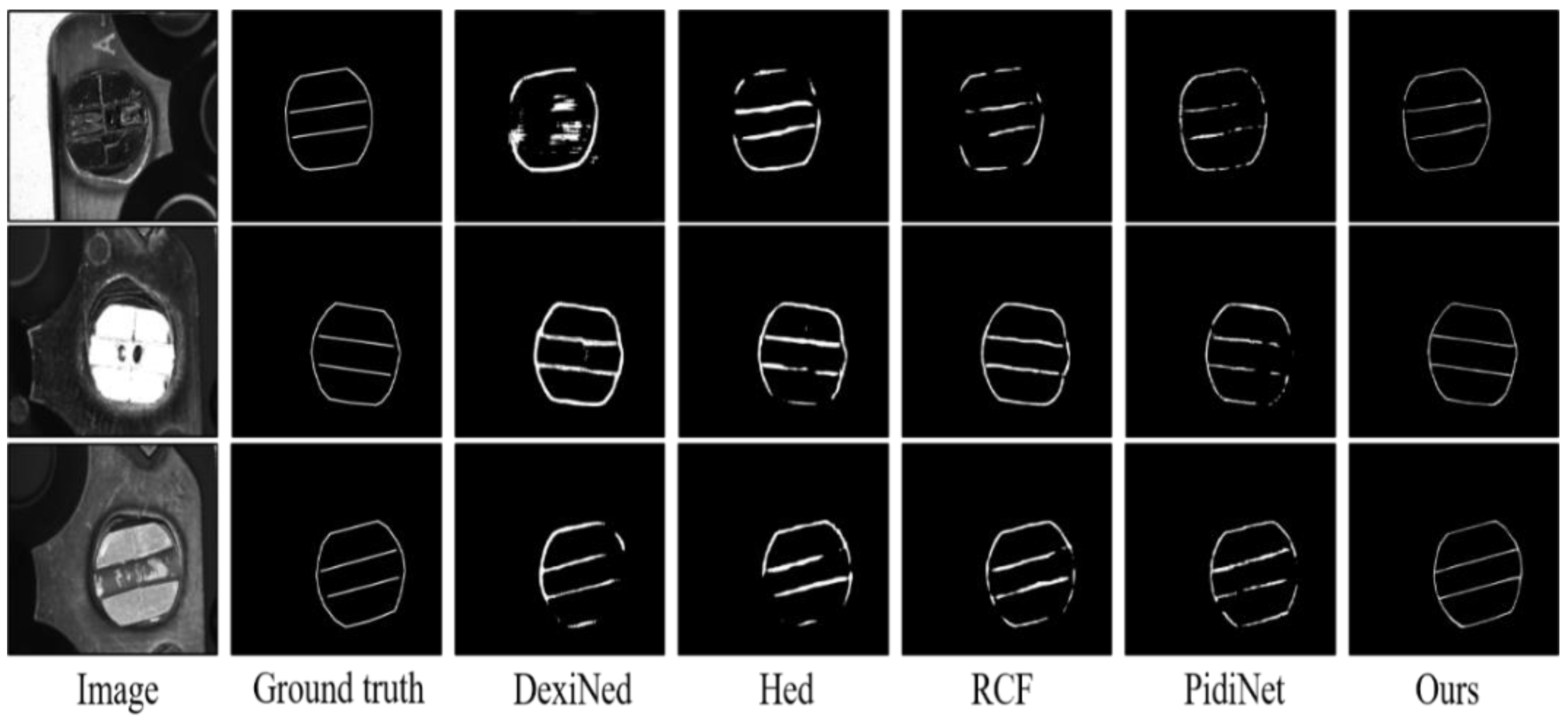
4.5. Experimental Results and Analysis
4.6. Ablative Study
5. Conclusions
Author Contributions
Funding
Institutional Review Board Statement
Informed Consent Statement
Data Availability Statement
Acknowledgments
Conflicts of Interest
Abbreviations
| GAN | Generative adversarial network |
| SVM | Support vector machine |
| CNN | Convolutional neural network |
| 2D | Two-dimensional |
| R-CNN | Region-based CNN |
| SENet | Squeeze and excitation network |
| FL | Focal loss |
| SA | Spatial attention |
| ODS | Optimal dataset scale |
| OIS | Optimal image scale |
| AP | Average precision |
References
- Hu, J.; Liu, S.; Liu, J.; Wang, Z.; Huang, H. Pipe pose estimation based on machine vision. Measurement 2021, 182, 109585. [Google Scholar] [CrossRef]
- Bai, X.; Fang, Y.; Lin, W.; Wang, L.; Ju, B.-F. Saliency-Based Defect Detection in Industrial Images by Using Phase Spectrum. IEEE Trans. Ind. Inform. 2014, 10, 2135–2145. [Google Scholar] [CrossRef]
- Ian, G.; Jean, P.-A.; Mirza, M.; Bing, X.; David, W.-F.; Sherjil, O.; Aaron, C.; Yoshua, B. Generative Adversarial Nets. Adv. Neural Inf. Process. Syst. 2014, 2, 2672–2680. [Google Scholar]
- Yu, F.; Koltun, V. Multi-Scale Context Aggregation by Dilated Convolutions. In Proceedings of the ICLR, San Juan, Puerto Rico, 2–4 May 2016. [Google Scholar]
- Huang, G.; Chen, J.; Liu, L. One-Class SVM Model-Based Tunnel Personnel Safety Detection Technology. Appl. Sci. 2023, 13, 1734. [Google Scholar] [CrossRef]
- Zhao, F.; Xu, L.; Lv, L.; Zhang, Y. Wheat Ear Detection Algorithm Based on Improved YOLOv4. Appl. Sci. 2022, 12, 12195. [Google Scholar] [CrossRef]
- Hwang, B.; Lee, S.; Han, H. DLMFCOS: Efficient Dual-Path Lightweight Module for Fully Convolutional Object Detection. Appl. Sci. 2023, 13, 1841. [Google Scholar] [CrossRef]
- Viola, P.; Jones, M. Rapid Object Detection Using a Boosted Cascade of Simple Features. In Proceedings of the 2001 IEEE Computer Society Conference on Computer Vision and Pattern Recognition, Kauai, HI, USA, 8–14 December 2001; Volume 1, pp. I–I. [Google Scholar]
- Gonzalez, R.C.; Woods, R.E. Wavelets and Multiresolution Processing. In Digital Image Processing, 3rd ed.; Prentice Hall: Upper Saddle River, NJ, USA, 2007; Volume 7, pp. 461–521. [Google Scholar]
- Dalal, N.; Triggs, B. Histograms of Oriented Gradients for Human Detection. In Proceedings of the Computer Vision and Pattern Recognition, San Diego, CA, USA, 20–26 June 2005; pp. 886–893. [Google Scholar] [CrossRef]
- Felzenszwalb, P.F.; Girshick, R.B.; McAllester, D.; Ramanan, D. Object Detection with Discriminatively Trained Part-Based Models. IEEE Trans. Pattern Anal. Mach. Intell. 2009, 32, 1627–1645. [Google Scholar] [CrossRef]
- Hearst, M.A.; Dumais, S.T.; Osuna, E.; Platt, J.; Scholkopf, B. Support Vector Machines. IEEE Intell. Syst. Their Appl. 1998, 13, 18–28. [Google Scholar] [CrossRef]
- Yu, W.X.; Xu, G.L. Connector Surface Crack Detection Method. Laser Optoelectron. Prog. 2022, 59, 1415015. [Google Scholar]
- Shan, Z.; Xin, M.; Di, W. Machine Vision Measurement Method of Tooth Pitch Based on Gear Local Image. J. Sci. Instrum. 2018, 39, 7. [Google Scholar]
- Hongjian, Z.; Ping, H.; Xudong, Y. Fault Detection of Train Center Plate Bolts Loss Using Modified LBP and Optimization Algorithm. Open Autom. Control Syst. J. 2015, 7, 1916–1921. [Google Scholar] [CrossRef]
- Otsu, N. A threshold selection method from gray-level histograms. IEEE Trans. Syst. Man Cybern. 1979, 9, 62–66. [Google Scholar] [CrossRef]
- Wellner, P. Interacting with paper on the DigitalDesk. Commun. ACM 1993, 36, 87–96. [Google Scholar] [CrossRef]
- Beucher, S.; Lantuejoul, C. Use of Watersheds in Contour Detection. In Proceedings of the International Workshop on Image Processing: Real-Time Edge and Motion Detection/Estimation, Rennes, France, 17–21 September 1979. [Google Scholar]
- LeCun, Y.; Bengio, Y.; Hinton, G. Deep learning. Nature 2015, 521, 436–444. [Google Scholar] [CrossRef]
- Jarrett, K.; Kavukcuoglu, K.; Ranzato, M.A.; LeCun, Y. What is the best multi-stage architecture for object recognition? In Proceedings of the 12th International Conference on Computer Vision Workshops, Kyoto, Japan, 27 September–4 October 2009; pp. 2146–2153. [Google Scholar] [CrossRef]
- Turaga, S.C.; Murray, J.F.; Jain, V.; Roth, F.; Helmstaedter, M.; Briggman, K.; Denk, W.; Seung, H.S. Convolutional Networks Can Learn to Generate Affinity Graphs for Image Segmentation. Neural Comput. 2010, 22, 511–538. [Google Scholar] [CrossRef]
- Bengio, Y.; Courville, A.; Vincent, P. Representation Learning: A Review and New Perspectives. IEEE Trans. Pattern Anal. Mach. Intell. 2013, 35, 1798–1828. [Google Scholar] [CrossRef] [PubMed]
- Dong, H.; Song, K.; He, Y.; Xu, J.; Yan, Y.; Meng, Q. PGA-Net: Pyramid Feature Fusion and Global Context Attention Network for Automated Surface Defect Detection. IEEE Trans. Ind. Inform. 2019, 16, 7448–7458. [Google Scholar] [CrossRef]
- Ge, J.H.; Wang, J.; Peng, Y.P.; Li, J.; Xiao, C.; Liu, Y. Recognition Method for Spray-Painted Workpieces Based on Mask R-CNN and Fast Point Feature Histogram Feature Pairing. Laser Optoelectron. Prog. 2022, 59, 1415016. [Google Scholar]
- He, K.; Gkioxari, G.; Dollar, P.; Girshick, R. Mask R-CNN. In Proceedings of the IEEE International Conference on Computer Vision, Venice, Italy, 22–29 October 2017. [Google Scholar]
- Li, J.X.; Qiu, D.; Yang, H.T.; Liu, K. Research on Workpiece Recognition Method Based on Improved YOLOv3. Modular Mach. Tool Autom. Manuf. Tech. 2020, 8, 92–96+100. [Google Scholar]
- Redmon, J.; Yolov, F.A. An Incremental Improvement. arXiv 2018, arXiv:1804.02767. [Google Scholar]
- Li, L.R.; Wang, Z.Y.; Zhang, K.; Yang, D.C.; Xiong, W.; Gong, P.C. Detection Algorithm of Train Bottom Parts Based on OSE-dResnet Network. Comput. Eng. Sci. 2022, 44, 692–698. [Google Scholar]
- Hu, J.; Shen, L.; Albanie, S. Squeeze-and-Excitation Networks. In Proceedings of the IEEE Conference on Computer Vision and Pattern Recognition, Salt Lake City, UT, USA, 18–22 June 2018; pp. 7132–7141. [Google Scholar]
- He, K.; Zhang, X.; Ren, S.; Sun, J. Deep Residual Learning for Image Recognition. In Proceedings of the of the 2016 Conference on Computer Vision and Pattern Recognition, Las Vegas, NV, USA, 26 June–1 July 2016; pp. 770–778. [Google Scholar]
- Lin, T.Y.; Dollár, P.; Girshick, R.; He, K.; Hariharan, B.; Belongie, S. Feature Pyramid Networks for Object Detection. In Proceedings of the 2017 IEEE Conference on Computer Vision and Pattern Recognition, Honolulu, HI, USA, 21–26 July 2017; pp. 936–944. [Google Scholar]
- Ren, S.; He, K.; Girshick, R.; Sun, J. Faster r-cnn: Towards Real-Time Object Detection with Region Proposal Networks. Adv. Neural Inf. Process. Syst. 2015, 28. [Google Scholar] [CrossRef]
- Redmon, J.; Divvala, S.; Girshick, R.; Farhadi, A. You Only Look Once: Unified, Real-Time Object Detection. In Proceedings of the IEEE Conference on Computer Vision and Pattern Recognition, Las Vegas, NV, USA, 26 June–1 July 2016; pp. 779–788. [Google Scholar]
- Liu, W.; Anguelov, D.; Erhan, D.; Szegedy, C.; Reed, S.; Fu, C.Y.; Berg, A.C. SSD: Single Shot Multibox Detector. In Proceedings of the European Conference on Computer Vision, Amsterdam, The Netherlands, 11–14 October 2016; Springer: Cham, Switzerland, 2016; pp. 21–37. [Google Scholar]
- Khan, A.; Chefranov, A.; Demirel, H. Image Scene Geometry Recognition Using Low-Level Features Fusion at Multi-layer Deep CNN. Neurocomputing 2021, 440, 111–126. [Google Scholar] [CrossRef]
- Woo, S.; Park, J.; Lee, J.Y.; Kweon, I.S. Cbam: Convolutional block attention module. In Proceedings of thes European Conference on Computer Vision (ECCV), Munich, Germany, 8–14 September 2018; pp. 3–19. [Google Scholar]
- Xie, S.; Tu, Z. Holistically Nested Edge Detection. In Proceedings of the IEEE International Conference on Computer Vision, Santiago, Chile, 11–18 December 2015; pp. 1395–1403. [Google Scholar]
- Liu, Y.; Cheng, M.M.; Hu, X.; Wang, K.; Bai, X. Richer Convolutional Features for Edge Detection. In Proceedings of the IEEE Conference on Computer Vision and Pattern Recognition, Honolulu, HI, USA, 21–26 July 2017; pp. 3000–3009. [Google Scholar]
- Soria, X.; Sappa, A.; Humanante, P.; Akbarinia, A. Dense Extreme Inception Network for Edge Detection. Pattern Recognit. 2023, 139, 109461. [Google Scholar] [CrossRef]
- Su, Z.; Liu, W.; Yu, Z.; Hu, D.; Liao, Q.; Tian, Q.; Liu, L. Pixel Difference Networks for Efficient Edge Detection. In Proceedings of the IEEE/CVF International Conference on Computer Vision, Montreal, QC, Canada, 11–17 October 2021; pp. 5117–5127. [Google Scholar]


| Layer | 1 | 2 | 3 | 4 | 5 | 6 | 7 | 8 | 9 | 10 |
|---|---|---|---|---|---|---|---|---|---|---|
| Name | Conv | Max-Pooling | Conv Block | Identity Block2 | Conv Block | Identity Block3 | Conv Block | Identity Block5 | Dilate Conv1 | Dilate Conv2 |
| Dilation size | 1 | 1 | 1 | 1 | 1 | 1 | 1 | 1 | 3 | 2 |
| Kernel size | 7 × 7 | 3 × 3 | 3 × 3 | (3 × 3)·2 * | 3 × 3 | (3 × 3)·3 * | 3 × 3 | (3 × 3)·5 * | 3 × 3 | 3 × 3 |
| Kernel receptive field | 7 × 7 | 3 × 3 | 3 × 3 | (3 × 3)·2 * | 3 × 3 | (3 × 3)·3 * | 3 × 3 | (3 × 3)·5 * | 7 × 7 | 5 × 5 |
| Stride | 2 | 2 | 1 | 1, 1 | 2 | 1, 1, 1 | 2 | 1, 1, 1, 1, 1 | 1 | 1 |
| Receptive field | 7 | 11 | 19 | 27, 35 | 43 | 59, 75, 91 | 107 | 139, 171, 203, 235, 267 | 363 | 427 |
| Method | ODS | OIS | AP | R50 |
|---|---|---|---|---|
| Hed | 0.9720 | 0.9835 | 0.9680 | 0.9775 |
| RCF | 0.9725 | 0.9860 | 0.9750 | 0.9885 |
| DexiNed | 0.9660 | 0.9735 | 0.9400 | 0.9905 |
| PidiNet | 0.9250 | 0.9540 | 0.9580 | 0.9960 |
| ours | 0.9740 | 0.9850 | 0.9775 | 0.9970 |
| Method | Center Point Accuracy | Maximum Error of Center Point (Pixel) | Angle Accuracy | Maximum Angle Error (Degree) |
|---|---|---|---|---|
| Hed | 94.7% | 18.27 | 97.2% | 2.86 |
| RCF | 96.5% | 12.68 | 98.4% | 2.93 |
| DexiNed | 93.6% | 13.45 | 92.7% | 4.99 |
| PidiNet | 95.2% | 14.31 | 96.4% | 3.56 |
| ours | 99.5% | 7.36 | 99.3% | 1.98 |
| Method | Center Point Accuracy | Angle Accuracy |
|---|---|---|
| Edge Network | 93.2% | 93.0% |
| Dilate | 98.7% | 98.6% |
| Refinement Edge | 99.5% | 99.3% |
Disclaimer/Publisher’s Note: The statements, opinions and data contained in all publications are solely those of the individual author(s) and contributor(s) and not of MDPI and/or the editor(s). MDPI and/or the editor(s) disclaim responsibility for any injury to people or property resulting from any ideas, methods, instructions or products referred to in the content. |
© 2023 by the authors. Licensee MDPI, Basel, Switzerland. This article is an open access article distributed under the terms and conditions of the Creative Commons Attribution (CC BY) license (https://creativecommons.org/licenses/by/4.0/).
Share and Cite
Feng, H.; Chen, X.; Zhuang, J.; Song, K.; Xiao, J.; Ye, S. Buckle Pose Estimation Using a Generative Adversarial Network. Appl. Sci. 2023, 13, 4220. https://doi.org/10.3390/app13074220
Feng H, Chen X, Zhuang J, Song K, Xiao J, Ye S. Buckle Pose Estimation Using a Generative Adversarial Network. Applied Sciences. 2023; 13(7):4220. https://doi.org/10.3390/app13074220
Chicago/Turabian StyleFeng, Hanfeng, Xiyu Chen, Jiayan Zhuang, Kangkang Song, Jiangjian Xiao, and Sichao Ye. 2023. "Buckle Pose Estimation Using a Generative Adversarial Network" Applied Sciences 13, no. 7: 4220. https://doi.org/10.3390/app13074220
APA StyleFeng, H., Chen, X., Zhuang, J., Song, K., Xiao, J., & Ye, S. (2023). Buckle Pose Estimation Using a Generative Adversarial Network. Applied Sciences, 13(7), 4220. https://doi.org/10.3390/app13074220