Abstract
For safety reasons, in order to ensure that a robot can make a reasonable response after a collision, it is often necessary to localize the collision. The traditional model-based collision localization methods, which are highly dependent on the designed observer, are often only useful for rough localization due to the bias between simulation and real-world application. In contrast, for fine collision localization of small-scale regions, data-driven methods can achieve better results. In order to obtain high localization accuracy, the data required by data-driven methods need to be as comprehensive as possible, and this will greatly increase the cost of data collection. To address this problem, this article is dedicated to developing a data-driven method for zero-shot collision localization based on local region data. In previous work, global region data were used to construct the collision localization model without considering the similarity of the data used for analysis caused by the assembly method of the contact parts. However, when using local region data to build collision localization models, the process is easily affected by similarity, resulting in a decrease in the accuracy of collision localization. To alleviate this situation, a two-stage scheme is implemented in our method to simultaneously isolate the similarity and realize collision localization. Compared with the classical methods, the proposed method achieves significantly improved collision localization accuracy.
1. Introduction
With the increasing popularity of electric vehicles (EVs), the charging of EVs has also attracted much attention. At present, the common charging method in public places involves a human taking the charger off the charging pile and then inserting the charger into the charging port of the EV. However, a charger with a heavy power cable usually brings great inconvenience to the users. In addition, unlike in traditional gas stations where each employee has undergone long-term training and the possibility of mis-operation during the refueling process is very small, in terms of charging electric vehicles, there is a potential safety hazard for the users who have not undergone strict training on how to use the charger by themselves. Therefore, in order to reduce the burden on users and eliminate potential safety hazards, the use of robots to automatically charge EVs has been proposed as an alternative solution [1,2,3].
Recently, research on the scenario of automatic charging for EVs has mainly focused on robot control, trajectory planning, and visual positioning of charging ports [4,5,6], while less attention has been paid to safety issues, even though safety is crucial during the automatic charging process. In general, in robot application scenarios, accidental contact or collision with the robot is the main safety concern. In order to deal with such problems, some research has explored utilizing a vision system to avoid accidental collisions [7,8,9]. However, such methods will fail in the blind spots of the system, and this situation is usually unavoidable in practice. Therefore, in order to improve the safety of robots, research on contact perception is necessary.
The contact or collision problem of robots is a very open problem for different application scenarios. These scenarios can be roughly divided into two categories based on whether humans and robots share the workspace or not. In the scenario where humans and robots share the workspace, human safety should be the focus. In this scenario, the threat of the robot to humans often comes from the link of the robot arm rather than the end effector. Considering this situation, it is possible to use model-based methods to analyze and detect the contact [10], determine whether the contact is intentional or accidental [11], and identify the location of the collision [12]. In addition, these works can provide a basis for planning the reasonable response of the robot after contact [13]. Due to the need to artificially set thresholds for the signals used in practice, the noise in different sensors and the complexity of the contact will influence the flexibility and robustness of the method. In the same scenario, the data-driven method is an alternative. For instance, in [14], an RNN-based model is used to realize collision classification. Similarly, in [15], a combination of the Generalized Momentum Observer and the NN method is used to realize the collision classification while also judging whether the collision occurred on the upper or lower part of the robot. However, because the motion of humans has a high degree of randomness, and different motion states of the robot will significantly affect the contact state, it is very difficult to obtain comprehensive contact data. This difficulty in obtaining comprehensive data can be referred to as mode difficulty in data acquisition. To alleviate the mode difficulty in this scenario, it is often necessary to assume that when the robot is in contact with the human, the human is quasi-static and the contact posture with the robot is fixed, and then the contact between the robot and the human is analyzed. However, these assumptions tend to weaken the practical effect of the method. In the other scenarios, where no shared workspace is required, in order to ensure that the robot is able to perform the manipulation tasks reasonably, the contact perception of the robot to the object is also needed. In contrast to the previous scenario, in order to perceive and grasp the objects in a reasonable pose, the contact localization of the end effector to the object is more important. Recent work has attempted to utilize tactile sensors for high-accuracy contact localization [16,17]. These tactile sensors are often mounted on specific end effectors, such as dexterous hands, U-shaped graspers, etc. Using a dense array arrangement on an extremely small surface area, the contact positioning accuracy of such a method can even reach the sub-millimeter level [16]. Nevertheless, in the scenario where the required contact frequency is high, the contact load is large, or there is an impact load, the sensor is likely to suffer from the memory effect upon making contact, resulting in a decrease in the robustness [18].
In the scenario of the automatic charging of EVs, with the development of automatic driving and automated valet parking (AVP), a large part of the automatic charging of electric vehicles in the future will be carried out in unmanned scenarios. In such an unmanned scenario, there is often no need to pay much attention to whether the robotic arm will threaten the safety of the surrounding people during its operation, and thus, ensuring the safety of the vehicle–robot interaction is more important. In general, in this scenario, for different types of robotic devices, the difficulty in end-effector contact analysis is different. The current charging robots for EVs can be divided into two types: the non-integrated charger type and the integrated charger type. In the non-integrated charger type, the charger and the robot are independent of each other. Before each charging, the robot needs to grab the charger from the charging pile. In the integrated charger type, the charger and the robot are connected, and the grabbing process of the charger can be omitted. Compared to the integrated charger type, using a robot to automatically grab the charger can result in a pose error of the charger. This error not only complicates the charging process but also makes contact analysis more difficult. Thus, the robots currently researched for automatic charging of electric vehicles are mainly charger-integrated [1,2,3]. Therefore, this work focuses on the contact problem of the charger-integrated robot. In our previous work, we explored the feasibility of using a supervised learning method to realize collision classification and collision localization for a charger-integrated, cable-driven manipulator when the charger and the charging port are in contact [19]. To alleviate the mode difficulty during data collection, we designed an mm scale area on the charging port and set pre-specified collision points in this region. Both the training set and the test set are these pre-specified collision points. The difference between the two sets is that the joint configurations, corresponding to the collision points at the same position in the specified region, are different. Using the above method, in order to localize a random collision point in such a region, the pre-specified collision points need to contain the random collision point. This will greatly increase the time needed for data collection in practical applications. In this work, to alleviate this situation, we explore an approach in which the entire region is divided into several sub-regions, and the pre-specified collision points in the sub-regions are used to predict the positions of collision points that have never been seen before. Here, we refer to these collision points that have never been seen before as zero-shot collision points. In the process of data collection, we found that when the central axis of the elastic compensator and the central axis of the end link of the manipulator do not coincide, the vibration caused by the collision between the charger and the upper part of the charging port will have a certain degree of similarity to the vibration caused by the collision between the charger and the lower part of the charging port. The main target of this article is to reduce the impact of that similarity on the localization results, while realizing zero-shot collision point localization, by proposing a two-stage collision localization scheme.
The rest of the paper is organized as follows. Section 2 reviews related works on collision localization. Section 3 describes the details of the datasets. Section 4 presents the architecture of our proposed method. Section 5 gives and discusses the experimental results, and Section 6 concludes the paper.
2. Related Work
As demonstrated in [20], the collision localization problem is essentially a classification problem. Unlike the collision classification task, which cares whether the collision is accidental or intentional, collision localization can be considered as a multi-classification problem with data acquisition boundary condition constraints. Collision localization often provides information for the subsequent collision response or assists in the completion of collision classification to improve the reliability of collision classification. Since the process of collision has temporal characteristics, this kind of classification problem can often be converted into a classification problem of time series signals.
Recently, related work has mainly used two types of signal-processing methods. One type consists of machine learning methods relying on manual feature extraction. In [20], the joint torque signal was collected in a specific motion mode, a variety of machine learning classifiers were used to filter out artificial features, and, finally, online collision classification was realized using NN and Bayesian decision theory. In [21], an artificial neural network was used to analyze the time domain and frequency domain characteristics of the vibration signal caused by the collision and then determine the collision localization from preset positions on different arms. Although this kind of method using artificial features is cheap in terms of classifier training and actual engineering application deployment, the manual extraction of features often relies on expert knowledge, and, when using such features, it is often impossible to update the corresponding features according to the classification results. When encountering complex problems, the effectiveness of such a method will decrease. In our previous work, we confirmed that using this kind of feature engineering method to deal with small-scale collision problems is not ideal. The other kind of method used in the literature is the automatic feature extraction method, which is capable of using raw data directly without prior feature engineering. The representative types are the RNN-based method and the CNN-based method. For example, in [14], the RNN-based method was used to solve the classification problem of distinguishing between intentional and accidental collisions between humans and robots, and it achieved good results. However, there are very few studies using RNN-based methods to explore the problem of robot collision localization. Theoretically, the RNN-based method has natural advantages for time-series signal processing; LSTM-based and GRU-based methods, especially, are widely used in EEG analysis [22], music emotion classification [23,24], and body pose estimation [25,26,27]. In our previous work, it was confirmed that the effect of using a two-layer CNN is slightly better than using LSTM when locating the pre-specified collision points. Therefore, CNN is used as the basis of this work.
Despite recent progress in collision localization using both artificial feature extraction and automatic feature extraction methods, there are still limitations in the existing studies. Most existing methods focus on large-scale collision localization problems, such as determining which link of the robot arm a collision occurred on. However, it is unclear whether these methods can be applied to small-scale collision problems, and the effectiveness of the signal used and the structure of the device must be considered. In some cases, it may be necessary to add external structures or sensors to the robot, and the suitability of the scenario used must also be considered. In our previous work, we proposed a data-driven method using external compensator vibration signals for studying small-scale collision localization problems in the context of electric vehicle automatic charging scenarios and achieved some success. However, our previous work mainly focused on studying the effect of the robot arm’s joint configuration and region partition schemes on collision localization and did not pay much attention to two additional crucial aspects of collision localization: (1) reducing the data collection cost required for data-driven collision localization methods and (2) suppressing the effects of signal similarity on collision localization caused by environmental factors. These are critical issues that need to be addressed to improve the accuracy and applicability of collision localization methods. Therefore, our current research focuses on addressing these two aspects of collision localization.
As demonstrated in Section 1, the asymmetric installation of the charger to the end of the manipulator will cause a similarity in the vibration signal of the compensator during a collision between the charger and the charging port. In general, the similarity may interfere with data-driven collision localization. However, there are very few current studies on how to reduce the impact of similarity on collision localization. In order to fill this gap, inspired by the divide-and-conquer method proposed in [28], before finely localizing the collision point, we first perform a rough localization on the collision point to distinguish whether the collision point is in the upper region or the lower region of the charging port. In addition, this can ensure that the overall approach has a better focus on the fine localization process. The main contributions of this paper are as follows:
- For the first time, we propose to use the vibration information from the elastic compensator corresponding to the pre-specified collision points to predict the location of the zero-shot collision point in the small-scale region, which helps to reduce the cost of data collection to some extent.
- Considering the similarity in the collision signal caused by the asymmetric installation of the end effector relative to the end link, a two-stage collision localization method is proposed. The rough localization stage of the method can reduce the effect of the vibration similarity and improve the ability of the classifier to produce promising results in the fine localization stage.
3. Dataset Description
3.1. Data Collection Scheme
In this work, a planar 3-DOF cable-driven manipulator with a slide platform at the bottom is used to perform a contact task. The vibration signal generated by the contact between the charger and the charging port is collected with an IMU mounted on the top of the charger. We use the collision point to represent the contact position where the charger meets the charging port. More details about the collection scheme can be found in our previous work [19]. In contrast to the previous work, the focus of this paper is mainly on the vulnerable domain, as shown in Figure 1. In the vulnerable domain, eight radial regions are set. Each region contains six collision points, and the point spacing is 1 mm. In the process of data collection, the influence of joint configuration and motion accuracy is also taken into account. Thus, data are collected multiple times at each collision point. After data cleaning, 5653 samples are generated. To simulate zero-shot collision, we randomly select a collision point from each region as the zero-shot collision point (indicated with the green point in Figure 1). These zero-shot collision points only appear in the test set and do not leak information during training. In this way, five cases of zero-shot collision points are designed as shown in Figure 1. The data distribution is shown in Table 1.
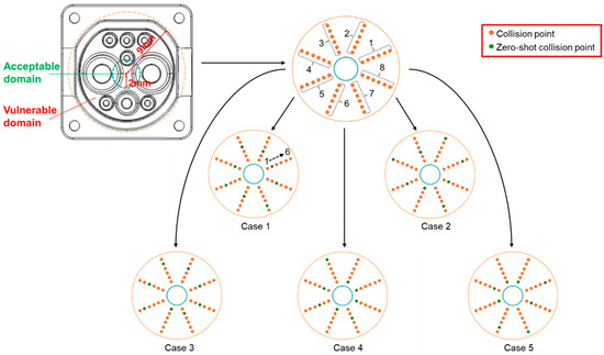
Figure 1.
The distribution of zero-shot collision points and collision points.

Table 1.
The total number of zero-shot collision points and collision points in different cases.
3.2. Segment and Labeling Scheme
As shown in Figure 2, the collected data contain 3-axis acceleration and 3-axis angular velocity. The sampling frequency is 1500 Hz. The data of different axes are synchronized in time. In our previous work, we proved that when the sampling frequency is 1500 Hz, setting the effective period to 267 ms can ensure that the collected vibration signals contain sufficient contact information. Thus, the effective period is set to 267 ms. In addition, to capture the transient characteristics of the collision without introducing too much irrelevant information, we set the pre-collision period to 20 ms. In the training and testing processes, the effective period of the signal is used as the input for the proposed method.
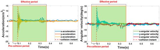
Figure 2.
The waveform of a collision point.
In terms of labeling, the actual physics of collisions should be considered. As shown in Figure 3, when the compensator is not collinear with the center line of the charger, the compensator will rotate in the same direction regardless of whether the collision occurs on the upper region or the lower region of the charging port. This will cause the vibration signals corresponding to the collision points of the upper and lower regions to be similar to some extent, and the purpose of the proposed two-stage method is to isolate this similarity to improve the positioning accuracy of the zero-shot collision points. For this consideration, in the first stage, data can be first labeled as U or L based on whether the collision point is in the upper or lower region. In the second stage, in order to predict which radial region the collision point will occur in, the data are labeled as R1 to R8, which is in the same order as shown in Figure 1. At this point, labels based on different annotation methods were established.
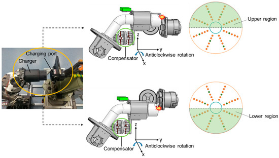
Figure 3.
The collision process between the charger and the charging port.
4. Proposed Two-Stage Collision Localization Method
In this section, our proposed method, a two-stage convolutional neural network, is introduced. In our scheme, the structure of the two-stage model is in binary tree form, and the results of the root stage will decide which leaf stage should be activated. Therefore, our method is called RL-CNN. Such a structure is designed to isolate regions where similar collision behavior occurs in order to improve localization accuracy. In the root stage, the task is to identify whether the collision happens in the upper region or the lower region. In the leaf stage, the model predicts in which fine-divided region the zero-shot collision point is located. As the whole area is partitioned into eight finely divided regions, the task in each leaf stage is essentially to solve a four-classification problem with zero-shot samples.
4.1. Baseline
CNN has been proved to be effective in numerous applications, such as brain tumor classification [29], hyperspectral images classification [30], remote sensing data classification [31], and so on. Due to the different application scenarios, there is an endless variety in variant structures of the CNN. Among the variants of CNNs, the classic models are: AlexNet [32], VGG [33], and ResNet [34]. AlexNet is mainly composed of five convolutional layers and two fully connected layers, and an innovative ReLU activation function was introduced into the structure. For most image classification problems, AlexNet has been proven to be effective. However, because it uses convolutional kernels with large sizes, when the network gets deeper, the computation burden is considerably increased. Compared to AlexNet, VGG uses 3 × 3 convolutional kernels to alleviate the problem above and proves that deeper networks generally have a stronger fitting ability. Although deep networks can achieve better results when dealing with complex image classification problems, merely increasing the depth of the network may be counterproductive. Essentially, a deep network that is built by simply stacking layers will face the problem of degradation. To solve this problem, ResNet utilizes skip connections to realize identity mapping with shallow networks. This method makes very deep network training possible. Although these methods have excellent performance in image classification, they may not be suitable for real-time application scenarios because too many network layers and too many parameters will increase the computational cost. In addition, when the input length is considerably longer than the width, with the increase in the number of network layers, the two-dimensional features will degrade into one-dimensional features, which leads to the degradation in the classification ability of the model. Therefore, we chose the structure proposed by our previous work as the baseline for both the root and leaf stages [19]. The details of the baseline structure are shown in Table 2.
Table 2.
The structure of the baseline.
4.2. Proposed RL-CNN Method
Figure 4 shows the proposed RL-CNN. After collecting data from IMU, the data will be segmented as described in Section 3, and then the segmented data will be normalized to [0, 1]. After the above preprocessing, we use the RL-CNN to perform the zero-shot collision point localization. In the root and leaf stages, the structures are similar. Their common parts consist of two convolutional layers, two max pooling layers, and three fully connected layers. The output of each convolutional layer will be batch normalized and then activated using the ReLU function. The purpose of using batch normalization in such a shallow network is to suppress the network’s over-understanding of visible data and improve the network’s ability to classify zero-shot data. For the same reason, a dropout layer is stacked after the first max pooling layer, and the rate is set to 0.5. In the root stage, the network is mainly used to distinguish whether the contact occurs in the upper region or the lower region of the charger. According to the output of the root stage, which leaf stage should be subsequently activated is determined. The only difference between the network used in the leaf stage and that used in the root stage is that the last layer in the network in the leaf stage uses a four-node fully connected layer with a softmax activation function. The leaf stages are mainly designed to estimate where the zero-shot collision point occurs in the finely divided region. For more details, the parameters of each layer are shown in Table 3.
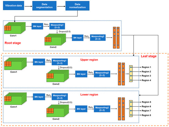
Figure 4.
The pipeline of the proposed zero-shot collision localization method.
Table 3.
The structure of the proposed RL-CNN.
In order to provide a more general understanding of RL-CNN, we present the mathematical analysis of RL-CNN. Since the two stages of RL-CNN are highly similar, for the sake of clarity, we focus on one of the stages here. For an input vibration signal of size (, , ), where , , and represent the length of the input, the width of the input, and the channel of the input, respectively, assuming that the kernel size of the convolutional layer is (, ), the channel in the convolutional layer is , the stride is , and then the feature extracted by the convolutional layer can be described as:
where and are the weight matrix and bias vector of the convolutional layer, respectively. In the convolution operation, the index and correspond to the spatial location of the output feature map. The index and represent the number of the input channel and the output channel, respectively. represents the activation function. Assuming the padding is , the output of the convolutional layer, denoted by , is a tensor of size (, , ), representing the activation maps of the convolutional layer. Among this process, the batch normalization is applied to the feature maps before the feature maps are activated to lead to improved accuracy and faster convergence during training.
In addition to the convolutional layer, we also incorporate a max pooling layer into our model. The max pooling operation is applied to each activation map independently, and when assuming the stride in the max pooling is also set as , the output of the max pooling layer is a tensor of size (, , ), where the pooling window size is (,). After the last max pooling layer, the output feature maps are flattened and passed through two or three fully connected layers. Finally, the output of the last fully connected layer is activated by the softmax activation function in order to serve as a criterion for collision localization.
When considering the time complexity of the proposed RL-CNN, it is necessary to analyze the time complexity of each component. Here, we need to consider the time complexity of the convolutional layers, batch normalization layers, max pooling layers, and fully connected layers. Compared to these four components, the impact of the activation functions on the overall time complexity can be neglected. When using the relevant parameters provided above and ignoring the influence of bias, the time complexity of the first convolutional layer can be expressed as:
When the network is relatively shallow and the number of filters in each convolutional layer is the same, the time complexity of the first convolutional layer can represent that of a generic convolutional layer in RL-CNN. The complexity of this component can be described as:
Based on similar reasons, the computational complexity of the batch normalization and max pooling layers can be expressed as follows, respectively:
Although the number of fully connected layers in the root and leaf stages is different, for the purpose of the time complexity analysis, we only need to consider the upper bound, which can be achieved by assuming that there are three fully connected layers. Let the number of nodes in these layers be , , and and let be the dimension of the flattened output from the last max pooling layer. Then, the time complexity of the fully connected layers can be expressed as:
Then, the overall time complexity of RL-CNN can be expressed as:
5. Experiment Results and Discussion
5.1. Experiment Results
In this work, we use the dataset described in Section 3 for the evaluation of the proposed methods. In this dataset, we only use collision point samples in different cases for training. In order to select the optimal model, the collision point samples are divided into a training set and a validation set, with a ratio of 8:2, and then the optimal parameters are selected according to the prediction accuracy of the model on the validation set. For testing, all of the zero-shot collision point samples from different cases are used, and the information from these samples will not be leaked during training. To illustrate the effectiveness of the proposed RL-CNN method, we compared the results with the baseline methods, both with and without batch normalization. For convenience, we named the baseline method using batch normalization as BN-DCNN, and the plain baseline method as DCNN. As mentioned in Section 2, since the RNN-based model has natural advantages for processing classification problems in time series, we also use LSTM, GRU, Bidirectional LSTM (BiLSTM), and Bidirectional GRU (BiGRU) as methods for comparison. All of these compared methods are trained in a similar way to the proposed method. However, it should be noted that since the compared methods only have one stage, the data for training the compared methods only needs radial region labels. To clearly describe the hyper-parameters of the mentioned methods, the relative settings are listed in Table 4.
Table 4.
The settings of the hyper-parameters of the proposed method and the compared methods.
Table 5 shows the prediction accuracy of different radial regions using the different methods. Each result is the average accuracy of five cross-validations. Overall, the accuracy of the proposed RL-CNN is higher than the compared methods in all cases. This is especially true in case 4; the proposed method has a considerable improvement over the next most accurate method (up to 7.77%), which is also the largest gap between the first and second place across all of the cases. Moreover, the addition of the BN layer makes the model better at predicting the location of zero-shot collision points than the shallow network without using the BN layer. For example, the average prediction accuracy of the CNN-BN method is 7.01% higher than that of the CNN method. Meanwhile, it is worth noting that the effect of the CNN-based model is better than that of the RNN-based model, which means that when the structure is relatively simple, the CNN-based model has more advantages for addressing the zero-shot collision problem. The experiments were performed using a Linux-based system equipped with an Intel (R) Core (TM) i7-10700K CPU @ 3.80 GHz, 31.9 GiB Memory, and an NVIDIA GeForce RTX 3080 GPU. Table 5 also presents the run time metrics for different models. Notably, the run time was measured with a batch size of 1.
Table 5.
The prediction accuracy of different radial regions.
Table 6 shows the F-score of each region for each different method. The results of each region are the average of the F-score from five cases. In terms of the F-score, the proposed RL-CNN is not always the best. For example, when predicting R1 samples, the CNN-BN method performs better than all other methods. In addition, although the RNN-based model has poor overall accuracy, it is more effective in locating the zero-shot collision points in some areas, such as R2 and R3. In these eight regions, the effect of all of the methods for localization of the zero-shot collision points in R4–R7 is obviously lower than that for localization of the zero-shot collision points in R1, R2, R3, and R8. Table 7 compares the localization effects of the different methods on the zero-shot collision points of the upper and lower regions. The proposed method still performs best in this binary classification task, for which the F-scores are as high as 94.53% and 93.60% for the upper region and the lower region, respectively. In contrast to the eight-region localization, there is a very small gap in the F-scores between the upper and lower regions. The highest gap is 0.92%, which happens when using RL-CNN.
Table 6.
The F-score of each radial region.
Table 7.
The F-score of the upper and lower regions.
5.2. Discussion
As shown in Table 5, there are obvious differences in the accuracy of predicting zero-shot collision points in different cases. Table 6 shows that the F-scores of R4–R7 are considerably lower than for other regions. Since this phenomenon exists with different models, it can be explained by flaws in the data. These flaws may be caused by the following two aspects: one is that there is vibration during the operation of the cable-driven manipulator, and the other is that the end faces of the charger and the charging port are not completely parallel. From the results, in a millimeter-level contact scenario, the deviation between the ideal collision point and the actual collision point caused by these two aspects will greatly affect the localization performance of the data-driven collision localization method. Unfortunately, due to structural characteristics, the vibration amplitude of the cable-driven manipulator is often larger than that of the joint direct-drive manipulator, and this vibration is often difficult to eliminate. In addition, in practical engineering applications, it is very difficult to ensure that the end faces of the charger and the charging port are parallel when collecting collision point data, especially when a large amount of data needs to be collected. Thus, the deviation is often unavoidable. As shown in Table 6, compared to other methods, the proposed method has better localization ability for these samples with high similarity, which is especially obvious in the case of eight-region localization. For example, in R4, the F-score of the proposed method is 95.25% higher than the next highest F-score. This, combined with the results in Table 7, can indicate that the root stage of the proposed method isolates the collision similarity caused by the asymmetric assembly of the compensator and the charger, which helps the method in the leaf stage to focus more on the localization of the finely divided regions. This scheme alleviates the impact of the deviation to a certain extent. In addition, by comparing the localization effects of DCNN and BN-DCNN in different regions of the collision points in Table 6 and Table 7, it can be seen that BN is effective in improving the network’s ability to locate zero-shot collision points. Although the zero-shot collision points and other collision points in the same region belong to the same class, there are obvious differences on the mm scale. Thus, the localization estimation of the zero-shot collision point requires the model to have good generalization ability. From the results, the introduction of the BN layer helps to improve the generalization ability of the localization model, and thus improves the model’s ability to localize zero-shot collision points.
6. Conclusions
In this article, we proposed a two-stage zero-shot collision localization method for the end-effector of the auto-charging manipulator using CNN and a regional division strategy called RL-CNN. The vibration signals in the elastic compensator (used to connect the charger to the end link of the manipulator) were used to train the proposed model. In order to explore the localization effect, we divided the end surface of the charging port into eight radial regions. In terms of simulating the zero-shot collision point, we selected one collision point from each region as the zero-shot collision point, and we ensured that the information on the zero-shot collision point was not leaked during the training process. The test results of the simulation experiment confirmed that the proposed method has a promising effect on zero-shot collision point localization. The conclusions may be summarized as follows:
- The proposed method has been proven to be able to achieve zero-shot collision localization in the millimeter-scale area. The method does not require complex prior expert knowledge, and the collision localization can be achieved using raw data, which is easier to implement in real application scenarios.
- The introduction of the root stage can effectively reduce the impact of the collision signal similarity caused by the non-central installation, and it helps the leaf stage to focus more on the finely divided subregions in each isolated region. This further enables the model to resist the loss in accuracy caused by the deviation between the collected collision point and the ideal collision point.
- By comparing the localization effects of BN-DCNN and DCNN in different finely divided regions, the use of BN in the shallow network structure is proven to be effective in improving the zero-shot collision localization accuracy of the model. The effect is more pronounced in regions with severe deviations.
Author Contributions
H.L. developed the methodology; H.L. and Y.L. conceived and designed the experiment; P.Q. and Z.L. conducted the data curation and collection; H.L. wrote the original draft of the paper; S.D. and D.W. reviewed and edited the paper. All authors have read and agreed to the published version of the manuscript.
Funding
This research received no external funding.
Institutional Review Board Statement
Not applicable.
Informed Consent Statement
Not applicable.
Data Availability Statement
The data mentioned in this paper are provided.
Conflicts of Interest
The authors declare no conflict of interest.
References
- Behl, M.; DuBro, J.; Flynt, T.; Hameed, I.; Lang, G.; Park, F. Autonomous Electric Vehicle Charging System. In Proceedings of the 2019 Systems and Information Engineering Design Symposium (SIEDS), Charlottesville, VA, USA, 26 April 2019; pp. 1–6. [Google Scholar]
- Asha Rani, G.S.; Lal Priya, P.S. Design of Automatic Charging System for Electric Vehicles Using Rigid-Flexible Manipulator. In Proceedings of the 2022 Second International Conference on Power, Control and Computing Technologies (ICPC2T), Raipur, India, 1–3 March 2022; pp. 1–6. [Google Scholar]
- Long, Y.; Wei, C.; Cao, C.; Hu, X.; Zhu, B.; Long, F. Design of High-Power Fully Automatic Charging Device. In Proceedings of the 2019 IEEE Sustainable Power and Energy Conference (iSPEC), Beijing, China, 21–23 November 2019; pp. 2738–2742. [Google Scholar]
- Lou, Y.; Di, S. Design of a Cable-Driven Auto-Charging Robot for Electric Vehicles. IEEE Access 2020, 8, 15640–15655. [Google Scholar] [CrossRef]
- Quan, P.; Lou, Y.; Lin, H.; Liang, Z.; Di, S. Research on Fast Identification and Location of Contour Features of Electric Vehicle Charging Port in Complex Scenes. IEEE Access 2022, 10, 26702–26714. [Google Scholar] [CrossRef]
- Quan, P.; Lou, Y.; Lin, H.; Liang, Z.; Wei, D.; Di, S. Research on Fast Recognition and Localization of an Electric Vehicle Charging Port Based on a Cluster Template Matching Algorithm. Sensors 2022, 22, 3599. [Google Scholar] [CrossRef] [PubMed]
- Scimmi, L.S.; Melchiorre, M.; Mauro, S.; Pastorelli, S.P. Implementing a Vision-Based Collision Avoidance Algorithm on a UR3 Robot. In Proceedings of the 2019 23rd International Conference on Mechatronics Technology (ICMT), Salerno, Italy, 23–26 October 2019; pp. 1–6. [Google Scholar]
- Nascimento, H.; Mujica, M.; Benoussaad, M. Collision Avoidance in Human-Robot Interaction Using Kinect Vision System Combined with Robot’s Model and Data. In Proceedings of the 2020 IEEE/RSJ International Conference on Intelligent Robots and Systems (IROS), Las Vegas, NV, USA, 24 October 2020; pp. 10293–10298. [Google Scholar]
- Fan, J.; Zheng, P.; Li, S. Vision-Based Holistic Scene Understanding towards Proactive Human–Robot Collaboration. Robot. Comput.-Integr. Manuf. 2022, 75, 102304. [Google Scholar] [CrossRef]
- Xiao, J.; Zhang, Q.; Hong, Y.; Wang, G.; Zeng, F. Collision Detection Algorithm for Collaborative Robots Considering Joint Friction. International J. Adv. Robot. Syst. 2018, 15, 172988141878899. [Google Scholar] [CrossRef]
- Popov, D.; Klimchik, A.; Mavridis, N. Collision Detection, Localization & Classification for Industrial Robots with Joint Torque Sensors. In Proceedings of the 2017 26th IEEE International Symposium on Robot and Human Interactive Communication (RO-MAN), Lisbon, Portugal, 28 August 2017; pp. 838–843. [Google Scholar]
- Vorndamme, J.; Schappler, M.; Haddadin, S. Collision Detection, Isolation and Identification for Humanoids. In Proceedings of the 2017 IEEE International Conference on Robotics and Automation (ICRA), Singapore, 29 May 2017; pp. 4754–4761. [Google Scholar]
- De Luca, A.; Albu-Schaffer, A.; Haddadin, S.; Hirzinger, G. Collision Detection and Safe Reaction with the DLR-III Lightweight Manipulator Arm. In Proceedings of the 2006 IEEE/RSJ International Conference on Intelligent Robots and Systems, Beijing, China, 9–15 October 2006; pp. 1623–1630. [Google Scholar]
- Lippi, M.; Gillini, G.; Marino, A.; Arrichiello, F. A Data-Driven Approach for Contact Detection, Classification and Reaction in Physical Human-Robot Collaboration. In Proceedings of the 2021 IEEE International Conference on Robotics and Automation (ICRA), Xi’an, China, 30 May 2021; pp. 3597–3603. [Google Scholar]
- Briquet-Kerestedjian, N.; Wahrburg, A.; Grossard, M.; Makarov, M.; Rodriguez-Ayerbe, P. Using Neural Networks for Classifying Human-Robot Contact Situations. In Proceedings of the 2019 18th European Control Conference (ECC), Naples, Italy, 25–28 June 2019; pp. 3279–3285. [Google Scholar]
- Piacenza, P.; Behrman, K.; Schifferer, B.; Kymissis, I.; Ciocarlie, M. A Sensorized Multicurved Robot Finger with Data-Driven Touch Sensing via Overlapping Light Signals. IEEE/ASME Trans. Mechatron. 2020, 25, 2416–2427. [Google Scholar] [CrossRef]
- Li, R.; Platt, R.; Yuan, W.; Ten Pas, A.; Roscup, N.; Srinivasan, M.A.; Adelson, E. Localization and Manipulation of Small Parts Using GelSight Tactile Sensing. In Proceedings of the 2014 IEEE/RSJ International Conference on Intelligent Robots and Systems, Chicago, IL, USA, 14–18 September 2014; pp. 3988–3993. [Google Scholar]
- Kappassov, Z.; Corrales, J.-A.; Perdereau, V. Tactile Sensing in Dexterous Robot Hands—Review. Robot. Auton. Syst. 2015, 74, 195–220. [Google Scholar] [CrossRef]
- Lin, H.; Quan, P.; Liang, Z.; Lou, Y.; Wei, D.; Di, S. Collision Localization and Classification on the End-Effector of a Cable-Driven Manipulator Applied to EV Auto-Charging Based on DCNN–SVM. Sensors 2022, 22, 3439. [Google Scholar] [CrossRef] [PubMed]
- Zhang, Z.; Qian, K.; Schuller, B.W.; Wollherr, D. An Online Robot Collision Detection and Identification Scheme by Supervised Learning and Bayesian Decision Theory. IEEE Trans. Automat. Sci. Eng. 2021, 18, 1144–1156. [Google Scholar] [CrossRef]
- Min, F.; Wang, G.; Liu, N. Collision Detection and Identification on Robot Manipulators Based on Vibration Analysis. Sensors 2019, 19, 1080. [Google Scholar] [CrossRef] [PubMed]
- Ariza, I.; Tardón, L.J.; Barbancho, A.M.; De-Torres, I.; Barbancho, I. Bi-LSTM Neural Network for EEG-Based Error Detection in Musicians’ Performance. Biomed. Signal Process. Control. 2022, 78, 103885. [Google Scholar] [CrossRef]
- Zhang, M.; Zhu, Y.; Ge, N.; Zhu, Y.; Feng, T.; Zhang, W. Attention-Based Joint Feature Extraction Model For Static Music Emotion Classification. In Proceedings of the 2021 14th International Symposium on Computational Intelligence and Design (ISCID), Hangzhou, China, 11–12 December 2021; pp. 291–296. [Google Scholar]
- Jia, X. Music Emotion Classification Method Based on Deep Learning and Improved Attention Mechanism. Comput. Intell. Neurosci. 2022, 2022, 5181899. [Google Scholar] [CrossRef] [PubMed]
- Nasiri, A.; Yoder, J.; Zhao, Y.; Hawkins, S.; Prado, M.; Gan, H. Pose Estimation-Based Lameness Recognition in Broiler Using CNN-LSTM Network. Comput. Electron. Agric. 2022, 197, 106931. [Google Scholar] [CrossRef]
- Kocabas, M.; Athanasiou, N.; Black, M.J. VIBE: Video Inference for Human Body Pose and Shape Estimation. In Proceedings of the 2020 IEEE/CVF Conference on Computer Vision and Pattern Recognition (CVPR), Seattle, WA, USA, 13–19 June 2020; pp. 5252–5262. [Google Scholar]
- Núñez, J.C.; Cabido, R.; Vélez, J.F.; Montemayor, A.S.; Pantrigo, J.J. Multiview 3D Human Pose Estimation Using Improved Least-Squares and LSTM Networks. Neurocomputing 2019, 323, 335–343. [Google Scholar] [CrossRef]
- Huang, J.; Lin, S.; Wang, N.; Dai, G.; Xie, Y.; Zhou, J. TSE-CNN: A Two-Stage End-to-End CNN for Human Activity Recognition. IEEE J. Biomed. Health Inform. 2020, 24, 292–299. [Google Scholar] [CrossRef] [PubMed]
- Ayadi, W.; Elhamzi, W.; Charfi, I.; Atri, M. Deep CNN for Brain Tumor Classification. Neural Process. Lett. 2021, 53, 671–700. [Google Scholar] [CrossRef]
- Chen, Y.; Jiang, H.; Li, C.; Jia, X.; Ghamisi, P. Deep Feature Extraction and Classification of Hyperspectral Images Based on Convolutional Neural Networks. IEEE Trans. Geosci. Remote Sens. 2016, 54, 6232–6251. [Google Scholar] [CrossRef]
- Xu, X.; Li, W.; Ran, Q.; Du, Q.; Gao, L.; Zhang, B. Multisource Remote Sensing Data Classification Based on Convolutional Neural Network. IEEE Trans. Geosci. Remote Sens. 2018, 56, 937–949. [Google Scholar] [CrossRef]
- Krizhevsky, A.; Sutskever, I.; Hinton, G.E. ImageNet Classification with Deep Convolutional Neural Networks. Commun. ACM 2017, 60, 84–90. [Google Scholar] [CrossRef]
- Simonyan, K.; Zisserman, A. Very Deep Convolutional Networks for Large-Scale Image Recognition. arXiv 2014, arXiv:1409.1556. [Google Scholar]
- He, K.; Zhang, X.; Ren, S.; Sun, J. Deep Residual Learning for Image Recognition. In Proceedings of the 2016 IEEE Conference on Computer Vision and Pattern Recognition (CVPR), Las Vegas, NV, USA, 26 June–1 July 2016; pp. 770–778. [Google Scholar]


Disclaimer/Publisher’s Note: The statements, opinions and data contained in all publications are solely those of the individual author(s) and contributor(s) and not of MDPI and/or the editor(s). MDPI and/or the editor(s) disclaim responsibility for any injury to people or property resulting from any ideas, methods, instructions or products referred to in the content. |
© 2023 by the authors. Licensee MDPI, Basel, Switzerland. This article is an open access article distributed under the terms and conditions of the Creative Commons Attribution (CC BY) license (https://creativecommons.org/licenses/by/4.0/).