Abstract
This paper studies frequency-limited model reduction for linear positive systems. Specifically, the objective is to develop a reduced-order model for a high-order positive system that preserves the positivity, while minimizing the approximation error within a given upper bound over a limited frequency interval. To characterize the finite-frequency specification and stability, we first present the analysis conditions in the form of bilinear matrix inequalities. By leveraging these conditions, we derive convex surrogate constraints by means of an inner-approximation strategy. Based on this, we construct a novel iterative algorithm for calculating and optimizing the reduced-order model. Finally, the effectiveness of the proposed model reduction method is illustrated with a numerical example.
1. Introduction
In various practical fields, such as biology, chemistry, economics and engineering, it is often the case that certain quantities are potentially constrained to be non-negative. The population of a species in an ecosystem [1], the transmission speed that a signal travels in network communication [2], and the distribution of light energy radiated by a light source, to mention a few. This property arises from physical or biological constraints that preclude negative values; the systems that exhibit the positivity are commonly referred to as positive systems whose state variables and output trajectories take non-negative values, provided that the excitation inputs and initial states are non-negative [3,4,5]. The study of positive systems can be traced back to the early 1990s when Berman [6] introduced the concept of positive matrices and their applications to linear systems. Later, the theory of linear systems was further developed. It has become a vibrant research area in control theory and systems engineering, including modeling and analysis [7], control and optimization [8,9,10,11], and its applications [12]. In many cases, high-order models are frequently encountered to provide exact characterizations of dynamical behaviors, which poses a significant challenge for the analysis and synthesis of the concerned systems [13]. Therefore, it is crucial to simplify models of dynamical systems by exploring lower-order models that approximate the original high-order ones according to certain criteria [14,15]. Various model reduction methods, such as balanced truncation [16], Hankel-norm reduction [17], and moment matching [18] have been developed.
For a specific positive system, it is reasonably required to preserve the positivity when employing model-reduction methods. Moreover, it suffices to satisfy given approximation specifications within limited frequency ranges [19]; it is especially relevant in engineering applications where practical constraints limit the operating frequency range. There are several model reduction approaches available to improve approximation performance over a limited frequency range, including methods such as frequency weighting [20] and frequency-specific balanced truncation [21]. Nevertheless, these methods cannot be directly applied to positive systems as they do not take the essential positivity of the reduced-order model into account. The generalized Kalman–Yakubovich–Popov (KYP) lemma is a powerful tool for characterizing the finite-frequency property, providing an equivalent condition for the solvability of frequency-limited specifications [22]. In the context of model reduction, this condition is expressed in a unified manner as a bilinear matrix inequality (BMI) involving coupled terms between two dependent decision variables [23]. To address this issue, some researchers have conservatively transformed the intractable BMI into a linear matrix inequality (LMI) by performing congruent transformation [24]. However, a potential drawback of this method is that the obtained LMI condition may always be infeasible. By alternately fixing one of the two coupled terms, D-K synthesis has been proposed to solve the BMI problems iteratively [25]; a major challenge of this approach lies in obtaining a feasible initial condition. Note that the introduction of additional positivity constraints and finite-frequency characterizations exacerbates the non-convexity, thereby making it difficult to explore a desired reduced-order model. Motivated by this, the paper aims to overcome this obstacle by developing a novel iterative procedure that can effectively solve the non-convex optimization problem.
In this paper, we aim to obtain a model with a lower order that preserves the positivity and captures the most significant behaviors within limited frequency intervals, which requires that the obtained model is positive and the resulting error system is stable with a given finite-frequency performance level. For this purpose, we establish conditions for the existence of such a reduced-order system in the form of BMIs. To address this problem, we propose a successive convex optimization (SCO) algorithm that iteratively solves a series of convex optimization sub-problems, each of which is an inner convex approximation of the original non-convex constraint. At each iteration, the solution to the previous step is used as a starting point for the next iteration until the convergence is reached. To summarize, this paper presents three contributions:
- A finite-frequency specification is employed to characterize the approximation error, improving the model reduction capability within limited frequency intervals.
- It is guaranteed that the reduced-order model maintains positivity, which retains the positive nature of the original system.
- An inner convexity strategy and associated SCO algorithm are proposed to obtain a desired reduced-order model without any parametrization techniques.
This paper is organized as follows: Section 2 introduces the problem statement and preliminary lemmas. Section 3 provides the conditions for the existence of a reduced-order model and a sequential algorithm for optimizing it. Section 4 gives an academic example to show the efficacy of the proposed method. Finally, Section 5 summarizes the contributions and discusses the limitations of the study and future work.
Notations: The symbols , , and represent the set of real numbers, n-dimensional column vectors, and -dimensional matrices, respectively. The notation refers to a set of column vectors with element-wise positive entries. The symbols and denote the identical and zero matrices, respectively. For , () means that M is positive-definite (negative-definite). , where is the transpose of M. Given a matrix , we use to signify that all the elements are non-negative (positive).
2. Problem Statement and Fundamental Results
Consider a stable system () with a relatively high order:
where are the state, input and output vectors, respectively, and are the given constant matrices. The model provides a unified description for linear systems, that is, for the continuous-time (CT) case and for the discrete-time (DT) case. Suppose that is a positive system whose definition is provided as follows:
Lemma 1
([26]). The system Σ is positive if all the state and output trajectories are non-negative, that is, and , provided that and .
Lemma 2
([19]). For the CT case, the system Σ is positive if, and only if, A is Metzler and , whereas, for the DT case, the system Σ is positive if, and only if, .
We intend to investigate an available model with a smaller order
for approximating with a sufficiently small error, where are reduced states and approximated outputs, respectively, and are unknown matrices. By defining and , the approximation error system can be expressed as
where
The transfer function of (3) is presented as:
where denote the Laplace operator for the CT case and the z operator for the DT case, respectively. For brevity, we give the following set to denote a positive system.
Definition 1.
The reduced-order system is positive if, and only if, , where
There are two concerns when developing a reduced-order model : First, it is expected that to preserve the positivity of . Second, in practical applications, it suffices to evaluate the approximation performance within a finite-frequency range. To provide an exact characterization for the property, we employ a frequency-limited specification
throughout the paper, where gives the frequency interval of interest, denotes the maximum singular value, and is an index to be minimized. Therefore, we summarize the overall problem formulation as follows:
Frequency-Limited Model Reduction: Given a specific frequency range , explore a reduced-order model such that
- The system is stable, and .
- The approximation error system satisfies the finite-frequency criterion in (6).
Next, we introduce the generalized KYP lemma, which is essential to the analysis of finite-frequency specifications.
Lemma 3

([22]). Given the state-space Equation (3) and a specific frequency range Ω, the system has a guaranteed criterion if, and only if, there exist symmetric matrices such that and
where , and Ξ concerning different frequency ranges are listed in Table 1.
Table 1.
with respect to different frequency ranges ().
Remark 1.
Lemma 3 provides an exact characterization for (6), which differs from the bounded real lemma and has the potential to improve the approximation capability with less conservatism. Notice that the condition for the solvability of limited-frequency performance is expressed as a BMI condition, which is difficult to solve due to the non-convexity, and it becomes even more arduous when an extra constraint is imposed.
3. Main Results
This section presents a method to design an appropriate reduced-order model. Firstly, an equivalent characterization for the system (3) is developed to parameterize the unknown matrices . Then, the design conditions in the form of BMIs are established, ensuring that the reduced-order model maintains positivity and the error system has a given finite-frequency performance level. On this basis, we propose an iterative procedure to obtain a reduced-order model.
To simplify the problem, we denote and
and, thus, (3) can be reformulated as . According to Remark 1, the condition (7) cannot be directly solved for which the constrained is coupled with P and Q. Therefore, we will provide feasible conditions in the following theorem.
Theorem 1.
Given a specified finite frequency range Ω and matrices , , a desired reduced-order model can be obtained if there exist matrices , such that and
where
Proof of Theorem 1.
By Lyapunov stability theory, the asymptotic stability of the reduced-order system (2) can be ensured if, and only if, there exists a Lyapunov matrix satisfying
and (7) can be further expressed as
Let , and its null space denoted as . Thus, (14) is equivalent to
By Finsler’s lemma, we have
where . It follows that (11) and (14) can be presented in a unified form of
where
It is observed that is coupled with . For given feasible matrices , we can reformulate (15) as
We notice that is linear, whereas is bilinear. According to [23], the bilinear term can be further decomposed into
where U serves as an auxiliary variable and , without loss of generality. Defining , and applying the above approximation strategy, results in
Similarly, we decompose U as , and thus
According to , one obtains that
which is equivalent to
We observe that is convex, implying for a given . Replacing with and performing the congruent transformation on (21), we can obtain (9) and (10). □
In Theorem 1, we first establish sufficient and necessary conditions (11) and (14) for the existence of a desired model in the form of BMIs. Given feasible solutions satisfying , the BMI conditions can be rewritten as the sum of linear and residual terms. By virtue of the convex-approximation strategy, we propose an SCO algorithm that iteratively solves a series of convex optimization sub-problems,
each of which is an inner convex approximation of the original non-convex constraint. At each iteration, the solution to the previous step is used as a starting point for the next iteration until the convergence is reached. To be concise, the above procedures can be summarized in the following algorithm.
Remark 2.
As pointed out in Algorithm 1, it is crucial to have an admissible for optimizing the subsequent solutions. However, one can see that obtaining such an initial condition is equally as intricate as solving the original problem. It can be shown that the objective function decreases with each iteration of the SCO algorithm, and according to the convergence property, we can obtain an initial solution by simply choosing a stable model . This significantly eases the challenge of implementing the proposed algorithm.
| Algorithm 1 SCO algorithm for calculating reduced-order models |
| Require: : tolerable bound; : maximal iteration limit |
| 1: Given a feasible solution , solve the convex optimization problem |
| to obtain the initial condition . Fix |
| 2: whiledo |
| 3: Solve (22) to the solution and optimum at -iteration. |
| 4: if then |
| 5: |
| 6: break; |
| 7: end if |
| 8: |
| 9: end while |
| 10: Result : the desired ; : optimal finite-frequency performance index. |
4. Simulation
In the simulation part, a system describing the compartmental network with two sub-systems is considered, and its state-space realization is given as follows:
The example is drawn from [19]. The restricted frequency is taken as rad/s. To develop a reduced-order model for approximating (24), we first adopt the initial condition as
Using the initial model and applying Algorithm 1, we optimize the reduced-order model as
with the optimal . By virtue of Lemma 2, it can be verified that the obtained reduced-order model (26) is positive. To validate the convergence property of the proposed algorithm, Figure 1 depicts the evolution of by configuring the maximum number of iterations and ignoring the tolerable bound . As shown in Figure 1, the proposed algorithm exhibits a monotonically decreasing trend in and converges to a fixed point eventually. Moreover, the result presents a significant improvement and provides a more exact approximation over the initial reduced-order model.
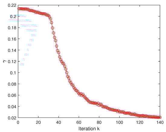
Figure 1.
Evolution by the proposed algorithm.
To illustrate the accuracy of (26) approximating (24), we provide Figure 2 and Figure 3 that demonstrate the singular value curves of with and , respectively. It can be observed that, in the given frequency range ( rad/s shaded region), the singular value curves of the reduced-order system closely match those of the original system , while the actual maximum singular values of the error system are strictly upper-bounded by . Based on the above analysis, one can conclude that the proposed reduced-order model is effective in approximating a high-order system with significant small errors.
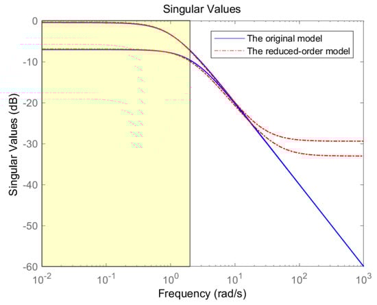
Figure 2.
Singular value curves of the original and reduced-order systems.
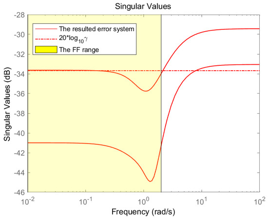
Figure 3.
Singular value curves of the associated error system.
5. Conclusions
This paper has considered the positivity-preserving model reduction for positive systems within limited frequency regions. To be specific, the positivity of the reduced-order model has been formulated as an element-wise positivity constraint, while the finite-frequency specification for the error system has been translated into BMI conditions. To provide a unified framework for addressing the BMI problems, we have proposed an SCO algorithm that serves as a promising solution for developing reduced-order models with positivity constraints and finite-frequency characterizations. Finally, the usefulness of the proposed method has been validated through a compartmental network example.
Author Contributions
Methodology, Y.R.; validation, Q.W.; writing—original draft preparation, Y.R.; writing—review and editing, Y.R. All authors have read and agreed to the published version of the manuscript.
Funding
This research was funded by the National Natural Science Foundation of China under Grant 62103041, and by the Postdoctoral Research Foundation of Shunde Innovation School, University of Science and Technology Beijing under Grant 2021BH010.
Institutional Review Board Statement
Not applicable.
Informed Consent Statement
Not applicable.
Data Availability Statement
Not applicable.
Conflicts of Interest
The authors declare no conflict of interest.
References
- Zhu, S.; Han, Q.L.; Zhang, C. l1-gain performance analysis and positive filter design for positive discrete-time Markov jump linear systems: A linear programming approach. Automatica 2014, 50, 2098–2107. [Google Scholar] [CrossRef]
- Shorten, R.; Wirth, F.; Leith, D. A positive systems model of TCP-like congestion control: Asymptotic results. IEEE/ACM Trans. Netw. 2006, 14, 616–629. [Google Scholar] [CrossRef]
- Van Den Hof, J. Positive linear observers for linear compartmental systems. SIAM J. Control. Optim. 1998, 36, 590–608. [Google Scholar] [CrossRef]
- Liu, J.J.R.; Kwok, K.W.; James, L. Decentralized H2 control for discrete-time neworked systems with positivity constraint. IEEE Trans. Neural Netw. Learn. Syst. 2023. [Google Scholar] [CrossRef]
- Fortuna, L.; Giuseppe, N.; Gallo, A. Model Order Reduction Techniques with Applications in Electrical Engineering; Springer Science & Business Media: Berlin, Germany, 2012. [Google Scholar]
- Berman, A.; Plemmons, R.J. Nonnegative Matrices in the Mathematical Sciences; SIAM: Philadelphia, PA, USA, 1994. [Google Scholar]
- Benner, P.; Ohlberger, M.; Cohen, A.; Willcox, K. Model Reduction and Approximation: Theory and Algorithms; SIAM: Philadelphia, PA, USA, 2017. [Google Scholar]
- Deaecto, G.S.; Geromel, J.C. H2 State Feedback Control Design of Continuous-Time Positive Linear Systems. IEEE Trans. Autom. Control. 2016, 62, 5844–5849. [Google Scholar] [CrossRef]
- Shen, J.; Lam, J. Static output-feedback stabilization with optimal L1-gain for positive linear systems. Automatica 2016, 63, 248–253. [Google Scholar] [CrossRef]
- Meng, A.; Lam, H.K.; Liu, F.; Yang, Y. Membership-Function-Dependent Design of l1-Gain Output Feedback Controller for Stabilization of Positive Polynomial Fuzzy Systems. IEEE Trans. Fuzzy Syst. 2022, 30, 2086–2100. [Google Scholar] [CrossRef]
- Xiao, S.; Ge, X.; Han, Q.L.; Zhang, Y. Distributed resilient estimator design for positive systems under topological attacks. IEEE Trans. Cybern. 2021, 51, 3676–3686. [Google Scholar] [CrossRef]
- Silva-Navarro, G.; Alvarez-Gallegos, J. Sign and stability of equilibria in quasi-monotone positive nonlinear systems. IEEE Trans. Autom. Control. 1997, 42, 403–407. [Google Scholar] [CrossRef]
- Breiten, T.; Unger, B. Passivity preserving model reduction via spectral factorization. Automatica 2022, 142, 110368. [Google Scholar] [CrossRef]
- Ibrir, S. A projection-based algorithm for model-order reduction with H2 performance: A convex-optimization setting. Automatica 2018, 93, 510–519. [Google Scholar] [CrossRef]
- Li, X.; Yin, S.; Gao, H. Passivity-preserving model reduction with finite frequency H∞ approximation performance. Automatica 2014, 50, 2294–2303. [Google Scholar] [CrossRef]
- Burohman, A.M.; Besselink, B.; Scherpen, J.M.A.; Camlibel, M.K. From Data to Reduced-order Models via Generalized Balanced Truncation. IEEE Trans. Autom. Control. 2023, 1–15. [Google Scholar] [CrossRef]
- Glover, K. All optimal Hankel-norm approximations of linear multivariable systems and their L∞-error bounds. Int. J. Control. 1984, 39, 1115–1193. [Google Scholar] [CrossRef]
- Astolfi, A. Model Reduction by Moment Matching for Linear and Nonlinear Systems. IEEE Trans. Autom. Control. 2010, 55, 2321–2336. [Google Scholar] [CrossRef]
- Li, X.; Yu, C.; Gao, H. Frequency-Limited H∞ Model Reduction for Positive Systems. IEEE Trans. Autom. Control. 2014, 60, 1093–1098. [Google Scholar] [CrossRef]
- Wu, F.; Jaramillo, J.J. Computationally efficient algorithm for frequency-weighted optimal H∞ model reduction. Asian J. Control. 2003, 5, 341–349. [Google Scholar] [CrossRef]
- Gugercin, S.; Antoulas, A.C. A survey of model reduction by balanced truncation and some new results. Int. J. Control. 2004, 77, 748–766. [Google Scholar] [CrossRef]
- Iwasaki, T.; Hara, S. Generalized KYP lemma: Unified frequency domain inequalities with design applications. IEEE Trans. Autom. Control. 2005, 50, 41–59. [Google Scholar] [CrossRef]
- Ren, Y.; Ding, D.W.; Li, Q.; Xie, X. Static Output Feedback Control for T–S Fuzzy Systems via a Successive Convex Optimization Algorithm. IEEE Trans. Fuzzy Syst. 2022, 30, 4298–4309. [Google Scholar] [CrossRef]
- Back, J.; Astolfi, A. Design of positive linear observers for positive linear systems via coordinate transformations and positive realizations. SIAM J. Control. Optim. 2008, 47, 345–373. [Google Scholar] [CrossRef]
- Li, P.; Lam, J.; Wang, Z.; Date, P. Positivity-preserving H∞ model reduction for positive systems. Automatica 2011, 47, 1504–1511. [Google Scholar] [CrossRef]
- Farina, L.; Rinaldi, S. Positive Linear Systems: Theory and Applications; John Wiley & Sons: Hoboken, NJ, USA, 2000. [Google Scholar]
Disclaimer/Publisher’s Note: The statements, opinions and data contained in all publications are solely those of the individual author(s) and contributor(s) and not of MDPI and/or the editor(s). MDPI and/or the editor(s) disclaim responsibility for any injury to people or property resulting from any ideas, methods, instructions or products referred to in the content. |
© 2023 by the authors. Licensee MDPI, Basel, Switzerland. This article is an open access article distributed under the terms and conditions of the Creative Commons Attribution (CC BY) license (https://creativecommons.org/licenses/by/4.0/).