Abstract
Infrared thermography techniques (IRT) are increasingly being applied in non-invasive structural defect detection and building inspection, as they provide accurate surface temperature (ST) and ST contrast (Delta-T) information. The common optional or off-the-shelf installation, of both low- and high-resolution thermal cameras, on commercial UAS further facilitates the application of IRT by enabling aerial imaging for building envelope surveys. The software used in photogrammetry is currently accurate and easy to use. The increasing computational capacity of the hardware allows three-dimensional models to be obtained from conventional photography, thermal, or even multispectral imagery with very short processing times, further improving the possibilities of analysing buildings and structures. Therefore, in this study, which is an extension of a previous work, the analysis of the envelope of a wine cellar, using manual thermal cameras, as well as cameras installed on board an Unmanned Aerial System (UAS), will be presented. Since the resolution of thermal images is much lower than that of conventional photography, and their nature does not allow for accurate representation of three-dimensional objects, a new, but simple, digital image pre-processing method will be presented to provide a more detailed 3D model. Then, the three-dimensional reconstruction, based on thermal imagery, of the building envelope will be performed and analysed. The limitations of each technique will be also detailed, together with the anomalies found and the proposed improvements.
Keywords:
UAS; IRT; thermal inspection; aerial inspection; 3D thermal photogrammetry; heat leaks; cellar; winery; thermal bridges 1. Introduction
Thermography, when applied in the field of construction, is mainly used for the non-invasive detection of pathologies in structures [1] and architectural heritage conservation, as presented in [2], where the extent of deterioration of limestone, in a monument dating back to the second half of the eighth century BC, was thoroughly studied [2]. Its use in the analysis of building envelopes is also well documented [3,4,5].
Infrared (IR) sensors can be effectively used to assess temperature distribution across surfaces, roofs, and walls. Two approaches have been widely implemented: passive and active. Passive methods consist of recording temperature without external heat stimulation, as the object itself acts as a thermal source. In [6], the restoration stones and original blocks (pyroclastic and travertine) used in Kuruçeşme Han in the city of Konya (Turkey) were examined in situ (infrared thermography, deep moisture meter, and ambient temperature meter), and in a laboratory (petrographic, index-mechanical, and thermal testing) environment. Active methods use an external heat stimulus to increase thermal contrast, making it more effective for detecting air infiltrations [7,8]. These procedures present some practical challenges, since environmental conditions may interfere with thermal flow, making them unsuitable for actual working conditions.
Passive IRT is typically associated with the analysis and the detection of potential anomalies in thermograms, showing defects in the envelope. This procedure is commonly applied in different types of building analysis and is frequently used to perform envelope study using a qualitative or quantitative approach. The aim is to evaluate the magnitude or importance of the target defects, so the measurement accuracy takes on special relevance [3,9].
Thermal audit campaigns require an in-depth study of the specific parameters linked to the properties of materials, such as emissivity and reflected apparent temperature (RAT) [4,10]. With changing environmental conditions, like ambient air temperature (AAT) and relative humidity (RH), not only thermal conductivity, but also specific heat and density of materials, vary, and this also influences in a significant way the heat transfer through buildings envelopes. Wind can also appreciably influence the heat losses through the envelope and the thermal measurements over the facades; therefore, it must be considered, too [11,12].
The thermography sector has undergone significant advances in recent years. The newest revolution in IRT comes from the democratisation of UAS technology and the emergence of lightweight devices easily installed on board. The integration of thermal sensors with drones opens up new possibilities for real-time aerial inspection in many fields. The massive capture capability of the UAS allows their application in thermal inspection of large areas such as in the agricultural field [13], hydrology [14] or industrial inspections, such as of photovoltaic farms [15,16,17].
However, the study of building envelopes is perhaps where the fusion of IRT and UAS technologies presents the most promising potential [18,19,20]. UAS-mounted thermal cameras can provide low-altitude aerial images, from a flexible perspective, with information on both qualitative and quantitative scenarios. For this reason, the method could be particularly well suited to inspecting difficult-to-access areas of the façade or the roof, where the thermal conductivity is higher than those areas with thermal bridges, air leakages or the presence of moisture in the walls.
Three-Dimensional Thermography
Three-dimensional thermography (3D-IRT) has been a growing field in recent years, with a particular focus on its application in building science. This growth is due to the fact that it allows the thermal behaviour to be analysed for use in thermal audits, providing complete information on the envelope as a whole, rather than a series of disconnected images. A three-dimensional reconstruction of the building envelope, although presenting some drawbacks, can provide both quantitative and qualitative information on thermal variations and, therefore, on the presence of defects. This approach, addressed in this study, still needs to be further developed since studies are scarce. In fact, ref. [21] identified a gap in the scientific literature related to the use of thermal imaging for building energy modelling and analysis.
In the last decade, very few scientific papers have been published on this topic, highlighting the potential of this technology for identifying and analysing thermal anomalies in buildings [22]. One of the main areas of research in 3D-IRT has been the development of new and improved algorithms for data processing and analysis, even in real time [23]. These algorithms have allowed more accurate and detailed analysis of thermal data to be obtained, making it possible to identify even small thermal anomalies that might otherwise have gone unnoticed.
Another area of research is the development of new hardware for 3D-IRT, including cameras and sensors that are capable of capturing high-resolution thermal data from a building’s exterior [24]. This has led to a greater understanding of the thermal behaviour of buildings, allowing for more accurate predictions of energy performance.
However, unlike RGB images, thermal images pose greater difficulties for correlation algorithms. Thermal images generally contain far fewer textural elements than conventional visible-band images; therefore, the tie point detection algorithms incorporated in SfM-MVS photogrammetry programs can fail with thermal images in complex 3D environments [25].
In fact, apart from the other analyses mentioned above, the main objective of this study is to present a simple but efficient thermal image pre-processing methodology which, to the authors’ knowledge, has never been applied before. With it, and despite the adverse conditions during the collection of images, which will be shown later, three-dimensional thermal models will be obtained that will demonstrate the advantages already mentioned.
One area where 3D-IRT has yet to be fully explored is in the application of this technology for understanding structures such as wine cellars. The unique thermal properties of these structures make them difficult to analyse using traditional methods, and a more detailed understanding of their thermal behaviour could lead to improved energy efficiency and better preservation of stored wines.
The aim of this study is to demonstrate how, by combining different techniques and tools—aerial photographs taken by low-cost thermal cameras on board a UAS, close-up images from hand-held cameras installed on a simple lifting device, development of three-dimensional thermal image models using photogrammetry, and installation of passive IR sensors—it is possible to detect thermal anomalies in building envelopes. Digital image pre-processing is proposed and applied to improve the 3D-IRT accuracy.
These procedures will be specifically applied to the wine cellar described in the following section. The results of the study will demonstrate that it is possible to detect issues that could compromise the wine aging process as well as taking the necessary corrective measures.
A 3D-IRT of the exterior of a wine cellar could provide valuable information on the thermal performance of the structure, including the location and extent of thermal bridges, areas of air leakage, and the presence of moisture in the walls. This information could then be used to make targeted improvements to the thermal envelope, leading to significant energy savings and improved wine storage conditions. Additionally, 3D-IRT could be used to monitor the thermal performance of the cellar over time, allowing for early detection of any issues that may arise.
2. Case Study
The experimental study was carried out in a winery built in O Saviñao (42°33′ N, 7°40′ W, altitude 399 m above Mean Seal Level (MAMSL) in the province of Lugo, Spain. The construction of the building dates back to 1920, when it was inaugurated for the production of local wines on a small scale. Since then, the building has undergone structural modifications and extensions, some of which were not documented. The results of these changes make its study of great interest, as it presents some singular structures and an important diversity of construction materials; the south façade is semi-buried to keep the AAT constant inside during all seasons of the year.
The exterior walls are mainly made of granite, and the doors, windows, and the structure supporting the roof are made of wood. Ceramic tiles were used for the wall cladding and the pillars and floor are built with bricks. Figure 1 shows the location of the winery and the exterior appearance of the building. Figure 2 shows a closer photograph of the exterior walls of the building and the interior.
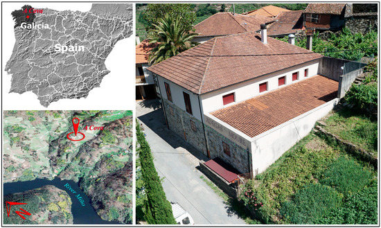
Figure 1.
On the left, geographic location of the winery; on the right, general view of the building.
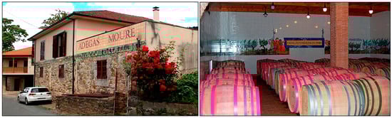
Figure 2.
On the left, the outer walls; on the right, the wine-ageing room (ground floor).
Temperature influences almost every step of wine production from the growing of the grape [26]. The process of wine maturation, which is particularly important, can be accelerated by high temperatures [27,28]. To prevent loss of quality, the wine should be stored at a cool cellar temperature [29,30]. The final wine quality can be controlled by monitoring the ambient air temperature inside the aging rooms [31], or even by means of sensors embedded inside wine barrels [32].
The introduction of modern cooling systems into the wine industry has allowed for the production of excellent wines almost anywhere in the world, regardless of the surrounding climate. However, energy use during wine production still represents a high percentage of the total electricity used by the winery [33]. Traditional cellars are more energy efficient than modern construction practices [34,35]. These traditional buildings incorporate bioclimatic strategies, such as the use of buried or semi-buried structures, adequate orientation, and natural ventilation [36,37].
Infrared thermography (IRT) techniques have been increasingly used in recent years due to their fast and reliable results in envelope inspection and their non-invasive nature [18]. This technology is adequate for evaluating thermal bridges, which are essential in energy audit procedures. Materials may not perform as expected, which is why mismatches between predicted and actual performance in buildings [38,39,40,41,42,43] are common.
Regarding the cellar where the study was carried out, it is important to point out that according to the Spanish Building Code CT-DB-HE [44], there are different climatic zones in the different regions of the country. This fact defines several wine production zones to which the so-called Denomination of Origin (DO) is assigned.
The winery studied corresponds to the Ribeira Sacra appellation. In this area of Spain, the AAT is 14 °C, and the average annual rainfall is 900 mm. This region has a microclimate with Mediterranean and continental influences due to its orography of steep slopes on the banks of the Miño and Sil rivers [45,46].
3. Materials and Methods
This section presents the instruments used in the study, together with their specifications and a brief introduction to the processing of thermal images using photogrammetry techniques to obtain three-dimensional models.
3.1. Electronic Instruments, Thermal Cameras, and UAS
The pieces of electronic equipment used for the measurement of temperature were the following:
- A Hobo data logger (model U12, Onset, MA, US) (with 4 × ext. channels) for measuring the AAT inside the wine cellars. It presents a 0.03 °C resolution and a +0.35 °C accuracy.
- Two Hobo data loggers (model U23-001 Pro v2) for measuring both indoor and outdoor ambient conditions (AAT and Relative Humidity (RH)). They present a 0.02 °C resolution with a +0.21 °C accuracy for AAT, and a 0.03% resolution and a +2.5% accuracy for RH.
- An XS Temp 7 portable thermometer (XS Instruments, Carpi, IT) equipped with a PT56C contact temperature probe to obtain ST measurements for cross-checking the thermal images radiometric measurements. The accuracy of this device is +0.15 °C (120 s).
The locations of the data loggers and the temperature probes will be presented below. Two radiometric thermal imaging cameras from FLIR™ Systems, USA were used for the non-contact measurement of the Surface Temperature (SF) of the walls in the wine cellar. The first, called FLIR Vue Pro-R 640, is lightweight and compact, designed to be installed on board a UAS. The second, the FLIR B335, is a conventional handheld camera. The former presents a resolution of 640 × 512 px, the maximum resolution that most UAS cameras allow without interpolation. The latter has a resolution of 320 × 240 px. The focal length of both cameras is 19 mm; pictures of both devices are shown in Figure 3.
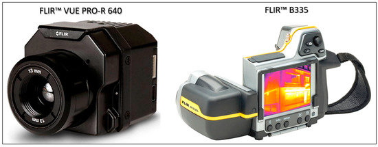
Figure 3.
Thermal cameras used during the study.
Two methods were used to record the images of the cellar walls. Firstly, the FLIR VUE Pro R camera was installed on a UAS called Quasar™, manufactured by the company Dronetools™-Sevilla. This 4-rotor aircraft has an autonomy of approximately 1 h carrying a payload of 1.2 kg. The thermal camera was installed together with a Sony™ mirrorless RGB camera, ILCE α6000™, of 24 MPx. Both were mounted on a gimbal that kept them stabilised. The shots from the two cameras were synchronised, and the video transmitter installed on board allowed real-time video streaming to a monitor on the ground. Although the UAS always remained within the line of sight (LOS), the above system provided real-time video streaming as if the flight were being carried out in first-person view (FPV), ensuring in this way that the region of interest (ROI) was correctly captured. The second procedure, much simpler than the previous one, consisted of using a telescopic tool composed of three parts: the first was a telescopic lifting mast built with lightweight materials and a maximum working length of 7 m. This mast was employed to raise the FLIR B335 ground camera. At the extreme of the mast, the second part was attached: a ball-head mount locked the camera solidly in the desired position. Finally, the ground control unit (GCU) also included FPV glasses and a shoot button, which were commercial devices directly wired to the camera. The GCU was designed to be operated by only one person. Figure 4 and Figure 5 show the UAS and the manual system respectively. The use of UAS and ground cameras allowed the study to be carried out redundantly by comparing the results obtained using both cameras.
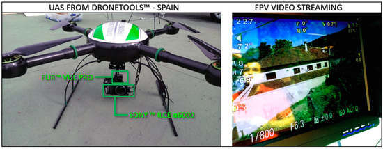
Figure 4.
UAS, on board cameras, and FPV system.
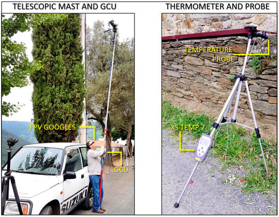
Figure 5.
Telescopic tool, GCU, thermometer, and probes.
3.2. Software and Fundamentals of SfM-MVS Photogrammetry
Structure from Motion Multiview Stereo (SfM-MVS) Photogrammetry is a cost-effective and versatile technique used, among other applications, for the three-dimensional (3D) modelling of terrain and the three-dimensional reconstruction of archaeological heritage sites and artistic objects [47,48,49].
The recording of overlapping images allows the use of SfM-MVS techniques. These procedures are considered to be automated photogrammetric methods characterised by high resolution and low cost [50], which are also flexible and easy to apply with a very fast learning curve [51]. The SfM-MVS is, in essence, based on the overlapping of the recorded images to find common points and thus generate a sparse three-dimensional point cloud, without the need for prior calibration [52]. To achieve this, it is necessary that the images present an adequate level of overlapping so that the processing software can identify homologous points between them [53]. Subsequently, MVS algorithms are applied to densify the sparse cloud from the already oriented images [54]. In addition, during image analysis, the software automatically determines the internal and external parameters of the camera [55]. It is important to note that one of the main advantages of photogrammetry techniques is the absence of invasiveness; only through image processing is it possible to detect damage and/or defects in the reconstructed structure or object, and to maintain a continuous monitoring of the evolution of the entire affected area [56].
SfM-MVS techniques allow the use of conventional (RGB), multispectral or thermal imagery. The first two are the most commonly used, although there are some studies in which terrain models have been constructed using thermal images [57]. In this study, SfM-MVS will not be applied to the terrain, but to the wine cellar.
Although various commercial products exist, one of the most widely used software packages in SfM-MVS is Agisoft Metashape™, largely due to its intuitive, user-friendly interface, and automated workflow, which allows for easy generation of dense point clouds, 3D models, digital elevation models, and orthomosaics.
The resolution of thermal cameras is significantly lower than that of RGB cameras, and since the three-dimensional reconstruction process is based on finding points belonging to two overlapping images, the modelling is much less detailed and more complex to perform. In addition, thermal imagery is affected by factors such as the emissivity of the materials, which makes it even more difficult to obtain a clear and detailed model. For this reason, the thermal images recorded by the cameras presented in the previous section were pre-processed using the Image Processing Toolbox belonging to MATLAB™. Figure 6 shows a diagram of the workflow and then details the focusing and contrast balancing techniques applied.
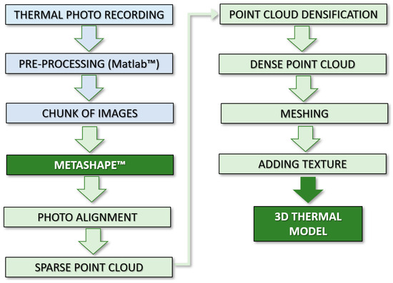
Figure 6.
Workflow for obtaining the three-dimensional model from thermal images.
As discussed above, one of the major difficulties in 3D building construction using thermal imaging is the low resolution of cameras designed to be used on board a UAS; 640 × 521 px compared to values as high as 6000 × 4000 px, and even higher on RGB high-resolution cameras. SfM-MVS techniques are based on the capture of photos with a good percentage of overlap that, as a whole, cover the entire region to be modelled. The reconstruction algorithms search for common points between the images, from which depth is introduced. A triangular mesh is then created, and finally a texture is added.
In the flowchart presented in Figure 6, the parts of the process that are carried out outside the photogrammetry software are coloured in blue and those that are carried out inside Metashape in green. It can be observed that after capturing the images, processing is required that does not apply to the RGB images. Although its mathematical foundations will be explained in detail in later sections, it can be anticipated that it mainly consists of the application of filters to eliminate noise or improve the focus of the images.
Once a body of photographs is available, it is uploaded into Metashape, where the first step consists of aligning the images, i.e., finding the common points (tie points) between them that generate a sparse point cloud. This initial point cloud is not dense enough to form a mesh to support the model. The SfM-MVS algorithms are again in charge of densifying it, until a dense point cloud has been obtained.
The meshing process consists of the creation of a mesh of triangular elements that join the points of the dense cloud. Once the mesh has been constructed, the three-dimensional model is visible. However, its surface does not have the texture of the real object or structure. In order for the final results to have the right texture, the pattern defined by the photographs is used. To facilitate the understanding of the process, Figure 7 shows 3 screenshots of the RGB model from the sparse point cloud to the final model.
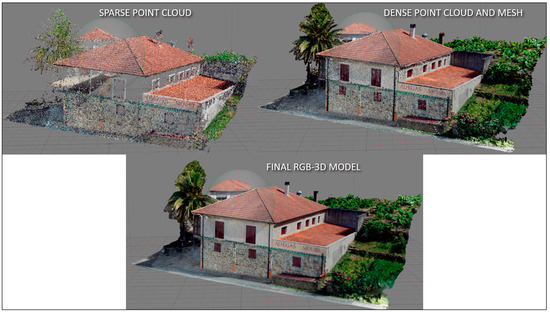
Figure 7.
Phases in the construction of the 3D-RGB model of the cellar.
3.3. Thermal Study of the Envelope: Probes and Cameras
In addition to the construction of the thermal model of the envelope, a complete interior and exterior survey of the walls was carried out. The thermal probes and the two cameras were used. Forty points were chosen at the same distance apart (300 mm). Twenty points correspond to the exterior walls and 20 points to the interior ones. All were labelled and selected from areas where no discontinuities existed. The thermometer was placed on top of each point to measure the surface temperature, and photographs were taken with the two thermal cameras, placed 3 m apart while keeping the point in the centre of the image. The results obtained are shown below: Figure 7 shows different views of the 3D model built with RGB images, Figure 8 shows the procedure for measuring the temperature of the walls using thermal probes and Figure 9 shows the thermal images with the sensitive points selected for the study.
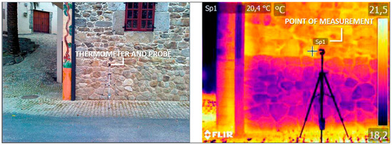
Figure 8.
Measurement procedure.
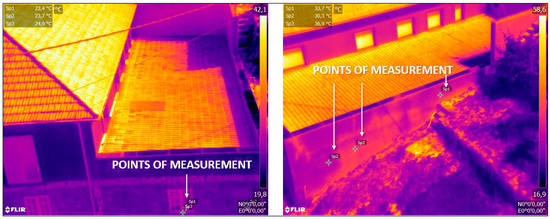
Figure 9.
Thermal images, points of measurement and anomalies (different colour patterns).
To check the validity of the study and to determine the accuracy that could be obtained by radiometric thermal imaging, the temperature values provided by the cameras at the reference points were compared with those obtained from the thermal probes in direct contact with the walls. The study was carried out for both cameras, inside and outside the envelope. Figure 10 and Figure 11 show, on the ordinate axis, the temperature measured by the probes, and on the abscissa axis, those obtained from the thermal images. Figure 10 shows the outside temperature results and Figure 11 shows the inside temperature results.
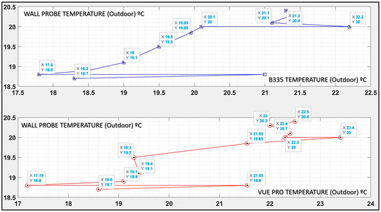
Figure 10.
Comparison between outdoor temperatures measured with the probes and those extracted from the two thermal cameras.
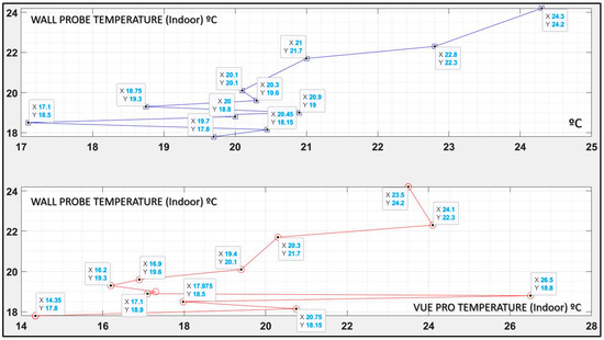
Figure 11.
Comparison between the indoor temperatures measured with the probes and those extracted from the two thermal cameras.
In order to check the validity of the radiometric measurements made with the two thermal cameras, the Pearson’s correlation coefficient was calculated between the matrices formed by the temperature values measured directly on the walls and the radiometric values. The correlation coefficient of two variables is a measure of their linear dependence. If each variable has N scalar observations, then the Pearson’s correlation coefficient (Equation (1)) is defined as [58]:
where μA and σA are the mean and standard deviation of A, and μB and σB are the mean and standard deviation of B. Alternatively, it is possible to define the correlation coefficient (Equation (2)) in terms of the covariance of A and B:
Table 1 shows the results obtained both indoors and outdoors with the two cameras. As can be seen, even in the case of the lowest correlation, the results are more than acceptable.

Table 1.
Correlation coefficients.
In the following, the procedure for the construction of the 3D thermal model will be presented. Then, the points or regions where anomalies were found will be highlighted, and finally, the conclusions and proposed improvements will be detailed.
3.4. 3D Thermal Model of the Envelope
Thermal cameras have a low resolution, meaning that at a certain distance from the object, the size of the pixel projected on it will be enlarged. The first consequence for a radiometric survey is that the measured temperature will be the average of the surface temperatures projected on each pixel.
On the other hand, this same problem appears in photogrammetric processing as the alignment of the images (extraction tie points) is much more complex. By approaching the recording of images from a UAS, a certain level of improvement could only be obtained with a minimum flight height and an increase in the overlapping of the photos. Reducing the height causes the footprint of the photo to be much smaller, increasing the number of photos noticeably, as does flying with greater overlap. The number of images that this solution would generate, apart from the inherent difficulty of the flight and its planning, means that the processing time would be extended to unacceptable limits or even require special hardware if it were to be processed in high or ultra-high quality.
The location of the building and its construction characteristics make it very difficult to take photographs from the UAS; not only is it impossible to photograph at close range, but there are also multiple obstacles that prevent the alignment of some of the photographs.
With all the limitations described so far, it was decided to carry out pre-processing of the images which, although simple, has not been applied to date, to the best of the authors’ knowledge. For this purpose, the MATLAB Toolbox was used, which offers all kinds of functions for the processing of RGB, thermal and multispectral images.
Although 3D models were constructed by applying different focusing techniques, white balance and histogram redistribution, as well as conversion of thermal images with colour palettes to greyscale, it is important to note that whatever method is used, the temperature, expressed in shades of grey and white, contained in the photograph must not be altered. That is, any noise reduction procedure, correction of the non-linearity of the camera’s thermal sensors or focusing cannot result in a model where thermal anomalies are diluted or delocalised.
In order to present the study as clearly as possible, several examples of photographs before and after processing are shown below, followed by details of the mathematical basis of the method used.
Figure 12 presents the conversion of a radiometric thermal image recorded with a colour palette to a greyscale image while retaining the thermal information. This transformation was performed to add to the set of photographs from which the model was generated, some taken by hand, thus making it possible to increase the size of the chunk loaded in Metashape.
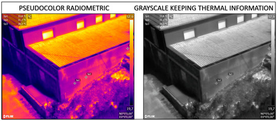
Figure 12.
Conversion to greyscale keeping thermal information.
As can be seen from Figure 13, some thermal images have a very uneven histogram that prevents the detection of tie points during photogrammetric processing. This figure shows the original photo on the left and on the right the same image after redistributing the histogram. Although the improvement in the result is clear and the resulting 3D model is valid and shows the sharpest geometric details, it was not used, because the redistribution of the histogram showed some thermal anomalies more intensely, but diluted the edges of the affected regions on the roof of the building.
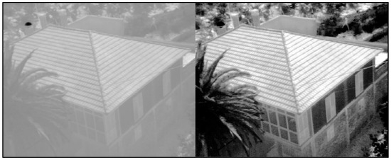
Figure 13.
Histogram equalisation. Left, original image; right, equalised.
Figure 14 and Figure 15 are of the greatest interest. They depict the application of two Gaussian filters with different depths. The first one, used in Figure 14, is of lower intensity than the one in Figure 15. In both cases, the better focus of the original image after applying the filter is evident. Since the final model was constructed after focusing the images and this type of filter is particularly suited to the characteristics of a thermal image, its mathematical foundations and properties are presented below. Its advantages for global and direct diagnosis, accuracy, processing complexity and computational time are also presented in later sections.
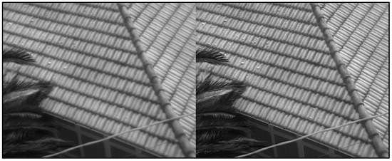
Figure 14.
Gaussian filter with minimum depth. Left, original image; right, focused.
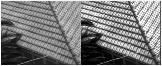
Figure 15.
Gaussian filter with maximum depth. Left, original image; right, focused.
To understand how the filter works, it is necessary to define what Gaussian noise is and what causes it to appear in RGB or thermal images. Gaussian noise, named after Carl Friedrich Gauss, is a term from signal processing theory denoting a kind of signal noise that has a probability density function (PDF) equal to that of the normal distribution (which is also known as the Gaussian distribution). In other words, the values that the noise can take are Gaussian-distributed. The probability density function p of a gaussian variable z (Equation (3)) is given by:
z being the grey level, µ the mean grey value, and σ the standard deviation.
The principal sources of Gaussian noise in digital images arise during acquisition, e.g., sensor noise caused by poor illumination and/or high temperature, and/or transmission of electronic circuit noise [59]. Gaussian noise can be reduced using a spatial filter, though when smoothing an image, an undesirable outcome may result in the blurring of fine-scaled image edges and details because they also correspond to blocked high frequencies. Conventional spatial filtering techniques for noise removal include mean (convolution) filtering, median filtering, and Gaussian smoothing. The three methods were tested and the Gaussian filter was selected as it improved the texture of the images, achieving the highest number of aligned thermograms.
The filter applied to the images was therefore a Gaussian low-pass filter in which it was possible to control the value of the standard deviation. This variable controls the size of the region around the edge pixels of the image that is affected by the sharpening.
By selecting the correct value, as in the photographs in Figure 14, there is no variation in the thermal information collected by the image and the improved focus allowed 199 images to be oriented, compared to the 153 that Metashape aligned before processing. Although the resulting model is not comparable to that extracted from the RGB images (6000 × 4000 px vs. 640 × 512) the areas of the walls and roof where thermal anomalies were measured are easily identifiable and the pre-processing valid for any three-dimensional reconstruction using thermal imagery.
Figure 16, Figure 17 and Figure 18 show three views of the thermal model. Figure 16 presents a zenithal view. It can be seen that in the main roof, in the central area where both sides converge, there is a central area and an outer area with different shades of grey, indicating the non-uniform distribution of temperatures. To maintain the thermal equilibrium of the envelope, the structure in these regions must be insulated.
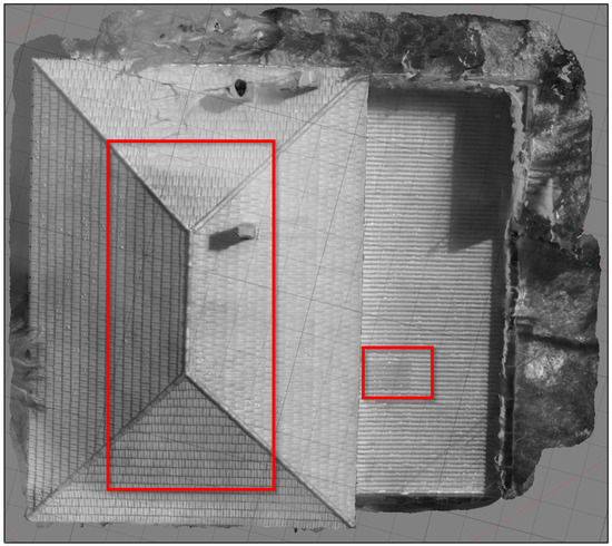
Figure 16.
Top view of the model, thermal anomalies in the roof.
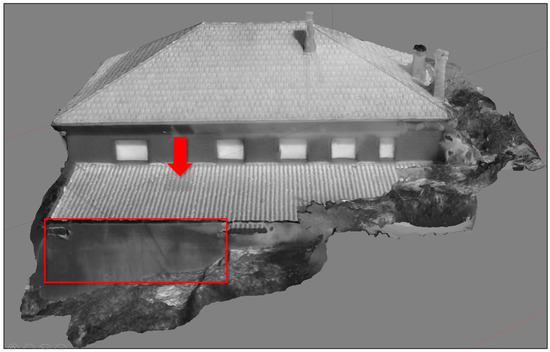
Figure 17.
Front view: thermal anomalies in the wall. The red arrow points to a small area with a thermal anomaly on the roof.
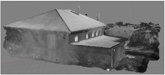
Figure 18.
Side view, even the most hidden wall is almost reconstructed.
Figure 17 is a front view of the model. In this image, it is possible to inspect the front wall on the left side. As in Figure 16, the temperature is not uniform, and the anomaly is also presented as a set of grey shades with different tones. In the region shown in the model within the red rectangle, the presence of moisture was detected.
The validity of the thermal model for obtaining an overall picture of the building envelope condition can be checked by simply reviewing Figure 1, Figure 2 and Figure 7. In the first two figures, it is clear how the wall shows stains caused by humidity. In Figure 7, one of the views of the 3D model constructed with the RGB images also shows the same pathology. Finally, Figure 18 is a side view of the model. Although it is impossible to make any kind of analysis here, it is presented to show how, even on the wall that is least likely to be photographed due to its position, which has a minimal projection towards the camera during the flight, it is almost possible to perform the reconstruction as well.
4. Conclusions and Corrective Actions
This study showed that IRT is a valid assessment method for envelopes and, in particular, for the wine cellar studied, where thermal stability is even more critical. Wine ageing is strongly affected by environmental factors; therefore, the detection of thermal insulation failures, heat leakage through joineries, and the presence of humidity must be identified and avoided.
The use of a UAS with an on-board camera has proven to be effective, especially in difficult-to-access areas such as the basement and roofs, reducing the risks related to performing an inspection.
The two cameras used showed excellent performance in detecting thermal anomalies, although they were somewhat more inaccurate when performing a radiometric assessment of the surface temperature; the measured temperature was particularly sensitive to the emissivity of the materials and to disturbances caused by specular reflections. During the study, it could be observed that for angles of more than 45°, the measurement deviation could exceed the sensitivity indicated by the camera manufacturer. Radiometry therefore requires further study and the use of more sophisticated cameras, but the qualitative assessment of defects was really effective. As a result of the study, the following corrective measures were proposed:
- Installation of systems for thermal bridge rupture in the joineries.
- Double-glazing windows.
- Reinforcement of the insulation layer in the subfloor.
- Cladding the concrete columns.
A key issue for the interpretation of the results of a thermal audit of buildings would be the use of photogrammetric products such as ortho-thermograms and/or 3D thermographic models. These products would provide a more holistic view than individual thermograms, yielding an interesting viewpoint to analyse the thermal performance of the building envelope as a whole. In fact, 3D-IRT provides a more useful product for evaluating the thermal performance of the winery and understanding its energy efficiency, as the building can be analysed from all directions.
Although the accuracy, analysed in terms of temperature values at the envelope walls cannot be assessed using the 3D-IRT model, it was shown in Section 3.1 that there is a more than acceptable level of error between the values measured by probes in contact with the walls and those obtained from thermal imaging at the same points. Furthermore, the comparison of the 3D RGB and thermal image models shows an excellent agreement in pinpointing the areas affected by moisture. Therefore, it can be stated that, although the exclusive use of 3D-IRT only allows the precise identification of the sensitive areas in a qualitative way, its accuracy is the same, in quantitative terms, as that demonstrated in the comparison referred to above. Pre-processing the thermal images not only increases the visual quality of the model, but also introduces a quantitative improvement in the number of thermograms that are aligned. In fact, 23.1% more images were aligned than by using the software directly. The pre-processing techniques (histogram balancing, Gaussian filtering, etc.) therefore allow for a more exhaustive and simple exploitation of the images collected by any UAS, thus facilitating a global and direct review of the areas in which the defects to be corrected are potentially found.
Some IRT cameras also include an RGB sensor that is capable of capturing simultaneous images with a geometry equivalent to or very close to that of the thermogram [60]. Optical image processing allows the camera positions to be determined and the scene geometry to be reconstructed and the temperature values to be superimposed or projected onto the 3D model [61]. However, this process also involves losing some of the radiometric temperature information at the pixel level. Therefore, there is still an important field of study in applying conventional SfM-MVS photogrammetry fluxes to thermal images in an efficient and reliable manner.
Author Contributions
M.G.-D.: Direction of the study, analysis of the data, proposal of corrective actions. J.O.S. and I.C.G.: Installation of on-board and hand-held measurement instruments, determination of critical analysis points, temperature data collection and photographic recording, data processing and correlation studies, proposal of corrective measures. M.F.C.: Construction of 3D models, both RGB and thermal, analysis of preprocessing tools to improve the quality of the thermal model, verification of the absence of distortions in the radiometry of the processed images, English revision of the document. All authors have read and agreed to the published version of the manuscript.
Funding
This study was partially funded by the Spanish Ministry of Economy and Competitivity (MINECO) under the COWINERGY project (BIA2014-54291-R) and for the Aids for consolidation and structuring of competitive research units in the universities of the Galician University System Ref. ED431B 2020/25.
Institutional Review Board Statement
Not applicable.
Informed Consent Statement
Not applicable.
Data Availability Statement
Not applicable.
Conflicts of Interest
The authors declare no conflict of interest.
References
- Titman, D.J. Applications of thermography in non-destructive testing of structures. NDT E Int. 2001, 34, 149–154. [Google Scholar] [CrossRef]
- Korkanç, M.; İnce, İ.; Hatır, M.E.; Tosunlar, M.B. Atmospheric and anthropogenic deterioration of the İvriz rock monument: Ereğli-Konya, Central Anatolia, Turkey. Bull. Eng. Geol. Environ. 2021, 80, 3053–3063. [Google Scholar] [CrossRef]
- Kirimtat, A.; Krejcar, O. A review of infrared thermography for the investigation of building envelopes: Advances and prospects. Energy Build. 2018, 176, 390–406. [Google Scholar] [CrossRef]
- Cerdeira, F.; Vázquez, M.; Collazo, J.; Granada, E. Applicability of infrared thermography to the study of the behaviour of stone panels as building envelopes. Energy Build. 2011, 43, 1845–1851. [Google Scholar] [CrossRef]
- Dufour, M.B.; Derome, D.; Zmeureanu, R. Analysis of thermograms for the estimation of dimensions of cracks in building envelope. Infrared Phys. Technol. 2009, 52, 70–78. [Google Scholar] [CrossRef]
- Hatır, M.E.; İnce, İ.; Bozkurt, F. Investigation of the effect of microclimatic environment in historical buildings via infrared thermography. J. Build. Eng. 2022, 57, 104916. [Google Scholar] [CrossRef]
- Lerma, C.; Barreira, E.; Almeida, R.M. A discussion concerning active infrared thermography in the evaluation of buildings air infiltration. Energy Build. 2018, 168, 56–66. [Google Scholar] [CrossRef]
- Taylor, T.; Counsell, J.; Gill, S. Energy efficiency is more than skin deep: Improving construction quality control in new-build housing using thermography. Energy Build. 2013, 66, 222–231. [Google Scholar] [CrossRef]
- Lai, W.W.-L.; Lee, K.-K.; Poon, C.-S. Validation of size estimation of debonds in external wall’s composite finishes via passive Infrared thermography and a gradient algorithm. Constr. Build. Mater. 2015, 87, 113–124. [Google Scholar] [CrossRef]
- Tejedor, B.; Casals, M.; Gangolells, M.; Roca, X. Quantitative internal infrared thermography for determining in-situ thermal behaviour of façades. Energy Build. 2017, 151, 187–197. [Google Scholar] [CrossRef]
- Sfarra, S.; Cicone, A.; Yousefi, B.; Ibarra-Castanedo, C.; Perilli, S.; Maldague, X. Improving the detection of thermal bridges in buildings via on-site infrared thermography: The potentialities of innovative mathematical tools. Energy Build. 2019, 182, 159–171. [Google Scholar] [CrossRef]
- Moyano-Campos, J.; Anton-García, D.; Rico-Delgado, F.; Martín-García, D. Threshold Values for Energy Loss in Building Façades Using Infrared Thermography Sustainable. In Sustainable Development and Renovation in Architecture, Urbanism and Engineering; Springer: Berlin/Heidelberg, Germany, 2017; pp. 427–432. [Google Scholar]
- Sagan, V.; Maimaitijiang, M.; Sidike, P.; Eblimit, K.; Peterson, K.T.; Hartling, S.; Esposito, F.; Khanal, K.; Newcomb, M.; Pauli, D.; et al. UAV-Based High Resolution Thermal Imaging for Vegetation Monitoring, and Plant Phenotyping Using ICI 8640 P, FLIR Vue Pro R 640, and Thermomap Cameras. Remote. Sens. 2019, 11, 330. [Google Scholar] [CrossRef]
- Khanal, S.; Fulton, J.; Shearer, S. An overview of current and potential applications of thermal remote sensing in precision agriculture. Comput. Electron. Agric. 2017, 139, 22–32. [Google Scholar] [CrossRef]
- Park, S.; Nolan, A.; Fuentes, S.; Hernandez, E.; Chung, H.; O’Connell, M. Estimation of crop water stress in a nectarine orchard using high-resolution imagery from unmanned aerial vehicle (UAV) Digital Vineyards View project Apple Sunburn Risk and Fruit Diameter Estimation Using a Smartphone App View project. In Proceedings of the 21st International Congress on Modelling and Simulation, Gold Coast, QLD, Australia, 29 November–4 December 2015. [Google Scholar]
- Aicardi, I.; Chiabrando, F.; Lingua, A.M.; Noardo, F.; Piras, M.; Vigna, B. A methodology for acquisition and processing of thermal data acquired by UAVs: A test about subfluvial springs’ investigations. Geomat. Nat. Hazards Risk 2016, 8, 5–17. [Google Scholar] [CrossRef]
- Fernández, A.; Usamentiaga, R.; De Arquer, P.; Fernández, M.Á.; Fernández, D.; Carús, J.L.; Fernández, M. Robust Detection, Classification and Localization of Defects in Large Photovoltaic Plants Based on Unmanned Aerial Vehicles and Infrared Thermography. Appl. Sci. 2020, 10, 5948. [Google Scholar] [CrossRef]
- Fox, M.; Coley, D.; Goodhew, S.; de Wilde, P. Thermography methodologies for detecting energy related building defects. Renew. Sustain. Energy Rev. 2014, 40, 296–310. [Google Scholar] [CrossRef]
- Nardi, I.; Lucchi, E.; de Rubeis, T.; Ambrosini, D. Quantification of heat energy losses through the building envelope: A state-of-the-art analysis with critical and comprehensive review on infrared thermography. Build. Environ. 2018, 146, 190–205. [Google Scholar] [CrossRef]
- Lucchi, E. Applications of the infrared thermography in the energy audit of buildings: A review. Renew. Sustain. Energy Rev. 2018, 82, 3077–3090. [Google Scholar] [CrossRef]
- Martin, M.; Chong, A.; Biljecki, F.; Miller, C. Infrared thermography in the built environment: A multi-scale review. Renew. Sustain. Energy Rev. 2022, 165, 112540. [Google Scholar] [CrossRef]
- Dlesk, A.; Vach, K.; Pavelka, K. Photogrammetric Co-Processing of Thermal Infrared Images and RGB Images. Sensors 2022, 22, 1655. [Google Scholar] [CrossRef] [PubMed]
- Landmann, M.; Heist, S.; Dietrich, P.; Lutzke, P.; Gebhart, I.; Templin, J.; Kühmstedt, P.; Tünnermann, A.; Notni, G. High-speed 3D thermography. Opt. Lasers Eng. 2019, 121, 448–455. [Google Scholar] [CrossRef]
- Kylili, A.; Fokaides, P.; Christou, P.; Kalogirou, S. Infrared thermography (IRT) applications for building diagnostics: A review. Appl. Energy 2014, 134, 531–549. [Google Scholar] [CrossRef]
- Hoffmann, H.; Nieto, H.; Jensen, R.; Guzinski, R.; Zarco-Tejada, P.; Friborg, T. Estimating evaporation with thermal UAV data and two-source energy balance models. Hydrol. Earth Syst. Sci. 2016, 20, 697–713. [Google Scholar] [CrossRef]
- Cancela, J.J.; Trigo-Córdoba, E.; Martínez, E.M.; Rey, B.J.; Bouzas-Cid, Y.; Fandiño, M.; Mirás-Avalos, J.M. Effects of climate variability on irrigation scheduling in white varieties of Vitis vinifera (L.) of NW Spain. Agric. Water Manag. 2016, 170, 99–109. [Google Scholar] [CrossRef]
- Ifie, I.; Abrankó, L.; Villa-Rodriguez, J.A.; Papp, N.; Ho, P.; Williamson, G.; Marshall, L.J. The effect of ageing temperature on the physicochemical properties, phytochemical profile and α-glucosidase inhibition of Hibiscus sabdaria (roselle) wine. Food Chem. 2018, 267, 263–270. [Google Scholar] [CrossRef]
- Styger, G.; Prior, B.; Bauer, F. Wine flavor and aroma. J. Ind. Microbiol. Biotechnol. 2011, 38, 1145–1159. [Google Scholar] [CrossRef]
- Bonfante, A.; Alfieri, S.M.; Albrizio, R.; Basile, A.; De Mascellis, R.; Gambuti, A.; Giorio, P.; Langella, G.; Manna, P.; Monaco, E.; et al. Evaluation of the effects of future climate change on grape quality through a physically based model application: A case study for the Aglianico grapevine in Campania region, Italy. Agric. Syst. 2017, 152, 100–109. [Google Scholar] [CrossRef]
- Crespo, J.; Rigou, P.; Romero, V.; García, M.; Arroyo, T.; Cabellos, J. Effect of seasonal climate fluctuations on the evolution of glycoconjugates during the ripening period of grapevine cv. Muscat à petits grains blancs berries. J. Sci. Food Agric. 2018, 98, 1803–1812. [Google Scholar] [CrossRef]
- Barbaresi, A.; Torreggiani, D.; Benni, S.; Tassinari, P. Indoor air temperature monitoring: A method lending support to management and design tested on a wine-aging room. Build. Environ. 2015, 86, 203–210. [Google Scholar] [CrossRef]
- Zhang, W.; Skouroumounis, G.K.; Monro, T.M.; Taylor, D. Distributed Wireless Monitoring System for Ullage and Temperature in Wine Barrels. Sensors 2015, 15, 19495–19506. [Google Scholar] [CrossRef]
- Correia, J.; Mourão, A.; Cavique, M. Energy evaluation at a winery: A case study at a Portuguese producer. In Proceedings of the IManE&E. MATEC Web of Conferences, Iasi, Romania, 24–27 May 2017; Volume 10001, pp. 1–9. [Google Scholar]
- Mazarrón, F.R.; Cid-Falceto, J.; Cañas-Guerrero, I. An assessment of using ground thermal inertia as passive thermal technique in the wine industry around the world. Appl. Therm. Eng. 2012, 33–34, 54–61. [Google Scholar] [CrossRef]
- Guerrero, I.C.; Ocaña, S.M. Study of the thermal behaviour of traditional wine cellars: The case of the area of “Tierras Sorianas del Cid” (Spain). Renew. Energy 2005, 30, 43–55. [Google Scholar] [CrossRef]
- Pardo, J.M.F.; Guerrero, I. Subterranean wine cellars of Central-Spain (Ribera de Duero): An underground built heritage to preserve. Tunn. Undergr. Space Technol. 2006, 21, 475–484. [Google Scholar] [CrossRef]
- Mazarrón, F.; Cañas-Guerrero, I. Seasonal analysis of the thermal behaviour of traditional underground wine cellars in Spain. Renew. Energy 2009, 34, 2484–2492. [Google Scholar] [CrossRef]
- Menezes, A.C.; Cripps, A.; Bouchlaghem, D.; Buswell, R. Predicted vs. actual energy performance of non-domestic buildings: Using post-occupancy evaluation data to reduce the performance gap. Appl. Energy 2012, 97, 355–364. [Google Scholar] [CrossRef]
- Guerra-Santin, O.; Tweed, C.; Jenkins, H.; Jiang, S. Monitoring the performance of low energy dwellings: Two UK case studies. Energy Build. 2013, 64, 32–40. [Google Scholar] [CrossRef]
- Demanuele, C.; Tweddell, T.; Davies, M. Bridging the gap between predicted and actual energy performance in schools. In Proceedings of the World Renewable Energy Congress XI, Abu Dhabi, United Arab Emirates, 25–30 September 2010; pp. 1–6. [Google Scholar]
- Bordass, B.; Cohen, R.; Field, J. Energy Performance of Non-Domestic Buildings: Closing the Credibility Gap. In 8th International Conference on Improving Energy Efficiency in Commercial Buildings; Building Performance Congress: London, UK, 2004; pp. 1–10. [Google Scholar]
- de Wilde, P. The gap between predicted and measured energy performance of buildings: A framework for investigation. Autom. Constr. 2014, 41, 40–49. [Google Scholar] [CrossRef]
- Trevisiol, F.; Barbieri, E.; Bitelli, G. Multitemporal Thermal Imagery Acquisition and Data Processing on Historical Masonry: Experimental Application on a Case Study. Sustainability 2022, 14, 10559. [Google Scholar] [CrossRef]
- Spain CTE-HE; Código Técnico de la Edificación. Basic document HE (Energy saving). June 2017, 68. Spanish Standard. Available online: https://www.codigotecnico.org/ (accessed on 10 March 2023).
- Fraga, H.; Malheiro, A.C.; Moutinho-Pereira, J.; Cardoso, R.M.; Soares, P.M.M.; Cancela, J.J.; Pinto, J.G.; dos Santos, J.A. Integrated Analysis of Climate, Soil, Topography and Vegetative Growth in Iberian Viticultural Regions. PLoS ONE 2014, 9, e108078. [Google Scholar] [CrossRef]
- Blanco-Ward, D.; García Queijeiro, J.M.; Jones, G.V. Spatial climate variability and viticulture in the Miño River Valley of Spain. Vitis J. Grapevine Res. 2007, 46, 63–70. [Google Scholar]
- Zollini, S.; Alicandro, M.; Dominici, D.; Quaresima, R.; Giallonardo, M. UAV Photogrammetry for Concrete Bridge Inspection Using Object-Based Image Analysis (OBIA). Remote Sens. 2020, 12, 3180. [Google Scholar] [CrossRef]
- Germanese, D.; Leone, G.R.; Moroni, D.; Pascali, M.; Tampucci, M. Long-Term Monitoring of Crack Patterns in Historic Structures Using UAVs and Planar Markers: A Preliminary Study. J. Imaging 2018, 4, 99. [Google Scholar] [CrossRef]
- Armesto, J.; Arias, P.; Roca, J.; Lorenzo, H. Monitoring and Assessing Structural Damage in Historic Buildings. Photogramm. Rec. 2008, 23, 36–50. [Google Scholar] [CrossRef]
- Tomás, R.; Riquelme, A.; Cano, M.; Abellán, A. Structure from Motion (SfM): Una Técnica Fotogramétrica de Bajo Coste Para la Caracterización y Monitoreo de Macizos Rocosos. En 10o Simposio Nacional de Ingeniería Geotécnica (pp. 209–2016). A Coruña. 2016. Available online: https://www.researchgate.net/publication/309611177_Structure_from_Motion_SfM_una_tecnica_fotogrametrica_de_bajo_coste_para_la_caracterizacion_y_monitoreo_de_macizos_rocosos (accessed on 10 March 2023).
- Gonçalves, G.; Gonçalves, D.; Gómez-Gutiérrez, Á.; Andriolo, U.; Pérez-Alvárez, J.A. 3D Reconstruction of Coastal Cliffs from Fixed-Wing and Multi-Rotor UAS: Impact of SfM-MVS Processing Parameters, Image Redundancy and Acquisition Geometry. Remote Sens. 2021, 13, 1222. [Google Scholar] [CrossRef]
- Narciso, E.M.; García, J.H.; Pérez-Alberti, A. Estudio de la Dinámica Geomorfológica Mediante la Obtención de Modelos Topográficos Históricos y Actuales a Partir de Fotogrametría Digital Automatizada: Acantilados de A Capelada (A Coruña, Galicia). En XIV Reunión de la Sociedad Española de Geomorfología. Málaga. 22–25 June 2016. Available online: https://www.researchgate.net/publication/308011087 (accessed on 10 March 2023).
- Souto-Vidal, M.; Ortiz-Sanz, J.; Gil-Docampo, M. Implementación del levantamiento eficiente de fachadas mediante fotogrametría digital automatizada y el uso de software gratuito. Inf. Construcción 2015, 67, e107. [Google Scholar] [CrossRef]
- Gil-Docampo, M.; Peña-Villasenín, S.; Ortiz-Sanz, J. An accessible, agile and low-cost workflow for 3D virtual analysis and automatic vector tracing of engravings: Atlantic rock art analysis. Archaeol. Prospect. 2020, 27, 153–168. [Google Scholar] [CrossRef]
- Aicardi, I.; Chiabrando, F.; Grasso, N.; Lingua, A.M.; Noardo, F.; Spanò, A. UAV Photogrammetry with Oblique Images: First Analysis on Data Acquisitionand Processing. Int. Arch. Photogramm. Remote Sens. Spat. Inf. Sci. 2016, XLI-B1, 835–842. [Google Scholar] [CrossRef]
- Grottoli, E.; Biausque, M.; Rogers, D.; Jackson, D.W.T.; Cooper, J.A.G. Structure-from-Motion-Derived Digital Surface Models from Historical Aerial Photographs: A New 3D Application for Coastal Dune Monitoring. Remote Sens. 2020, 13, 95. [Google Scholar] [CrossRef]
- Lagüela, S.; Díaz−Vilariño, L.; Roca, D.; Lorenzo, H. Aerial thermography from low-cost UAV for the generation of thermographic digital terrain models. Opto-Electron. Rev. 2015, 23, 76–82. [Google Scholar] [CrossRef]
- Press, W.H.; Teukolsky, S.A.; Vetterling, W.T.; Flannery, B.P. Numerical Recipes in C, 2nd ed.; Cambridge University Press: Cambridge, UK, 1992. [Google Scholar]
- Barbu, T. Variational Image Denoising Approach with Diffusion Porous Media Flow. Abstr. Appl. Anal. 2013, 2013, 856876. [Google Scholar] [CrossRef]
- Pant, S.P.; Nooralishahi, N.P.; Avdelidis, C.; Ibarra-Castanedo, M.; Genest, S.; Deane, J.J.; Valdes, A.; Zolotas, A.; Maldague, X. Evaluation and Selection of Video Stabilization Techniques for UAV-Based Active Infrared Thermography Application. Sensors 2021, 21, 1604. [Google Scholar] [CrossRef]
- Shariq, M.H.; Hughes, B.R. Revolutionising building inspection techniques to meet large-scale energy demands: A review of the state-of-the-art. Renew. Sustain. Energy Rev. 2020, 130, 109979. [Google Scholar] [CrossRef]


Disclaimer/Publisher’s Note: The statements, opinions and data contained in all publications are solely those of the individual author(s) and contributor(s) and not of MDPI and/or the editor(s). MDPI and/or the editor(s) disclaim responsibility for any injury to people or property resulting from any ideas, methods, instructions or products referred to in the content. |
© 2023 by the authors. Licensee MDPI, Basel, Switzerland. This article is an open access article distributed under the terms and conditions of the Creative Commons Attribution (CC BY) license (https://creativecommons.org/licenses/by/4.0/).