Abstract
Teacher job satisfaction is an important aspect of academic performance, student retention, and teacher retention. We propose to determine the predictive model of job satisfaction of basic education teachers using machine learning techniques. The original data set consisted of 15,087 instances and 942 attributes from the national survey of teachers from public and private educational institutions of regular basic education (ENDO-2018) carried out by the Ministry of Education of Peru. We used the ANOVA F-test filter and the Chi-Square filter as feature selection techniques. In the modeling phase, the logistic regression algorithms, Gradient Boosting, Random Forest, XGBoost and Decision Trees-CART were used. Among the algorithms evaluated, XGBoost and Random Forest stand out, obtaining similar results in 4 of the 8 metrics evaluated, these are: balanced accuracy of 74%, sensitivity of 74%, F1-Score of 0.48 and negative predictive value of 0.94. However, in terms of the area under the ROC curve, XGBoost scores 0.83, while Random Forest scores 0.82. These algorithms also obtain the highest true-positive values (479 instances) and lowest false-negative values (168 instances) in the confusion matrix. Economic income, satisfaction with life, self-esteem, teaching activity, relationship with the director, perception of living conditions, family relationships; health problems related to depression and satisfaction with the relationship with colleagues turned out to be the most important predictors of job satisfaction in basic education teachers.
1. Introduction
Studying the different aspects related to the teacher continues to be important. One of these is job satisfaction, which is found within the emotional dimension [1]. It is important to mention that in the educational field the highest rates of stress, anxiety and irritability have been found to affect the level of teachers’ job satisfaction [2]. Teacher job satisfaction is considered a key factor in the effectiveness not only of themselves, but also of the students, the school environment and the educational system in general [3,4]. It is currently known that satisfaction or dissatisfaction of the teachers with their work life could have a determining impact on the quality of teaching and student achievement [5,6,7,8].
In Peru, according to the Ref. [9], 42.1% of teachers have a regular level of satisfaction, that is, they have a low positive attitude about their work. In this scenario, it is of utmost importance to conduct studies to better understand the job satisfaction of teaching professionals, using current methods and tools. In line with this idea, the Ref. [10] recommends conducting studies that allow the analysis of how to avoid the lack of satisfaction in order to favor the non-appearance of burnout and demotivating symptoms in teachers. Studies close to this problem have been employing machine learning techniques, such as logistic regression, random forests, decision trees, AdaBoost algorithm, K-Nearest Neighbors, support machines, Naive Bayes with great success in the prediction of employee desertion in several organizations [11,12,13].
These techniques are also being employed to explore and discover reliable predictors in large volumes of data, with a large number of dimensions [14]. It is also possible to find factors affecting employee job satisfaction using Gradient boosting and Random Forests algorithms [15]. Another study developed by the Ref. [16] demonstrates the use of artificial neural networks to find the association between demographic variables, coaching leadership and job satisfaction of elementary school teachers in Korea with better results than multiple regression. Prediction of employee job satisfaction was also addressed using deep neural networks [17], decision tree algorithm (CART) and neural networks [18].
Although there are important advances in this area, most of them address job satisfaction in a more general way, on the other hand, there are studies that attempt to explain teacher job satisfaction using techniques such as linear hierarchical models [19], structural equation modeling [20], and analysis of variance (ANOVA) [21].
The contributions of this research are:
- We determined that the XGBoost and Random Forest algorithms allow us to obtain predictive models of job satisfaction of Peruvian basic education teachers with a balanced accuracy of 74%, sensitivity of 74%, F1-Score of 0.48, negative predictive value of 0.94, higher values of true-positives (479 instances) and lower values of false-negatives (168 instances). These values are unprecedented in the prediction of job satisfaction of basic education teachers in Peru.
- We were able to identify that the economic income, the satisfaction with: life, self-esteem, pedagogical activity and relationship with the director, in addition to perception of living conditions, satisfaction with their family relationships, problem of depression-related health and relationship satisfaction with colleagues turned out to be the most important variables in predicting teachers’ job satisfaction.
- Finally, we made available to the scientific community a set of pre-processed data with 13,302 records, 11 predictive columns and 1 to predict, to perform replicate experiments with other machine learning algorithms. We obtained these columns after the feature selection process applied to the original data set, which initially had 15,087 records and 942 columns.
2. State-of-the-Art
Below, we present recent related studies:
In the Ref. [22] the effect of principal support on teacher turnover intention in Kuwait was studied. The researchers used the technique of structural equations. Their results suggest that the principal’s support is desirable and positively affects teachers’ job satisfaction.
In the study by the Ref. [23], they analyzed the role of emotional regulation traits and satisfaction with life in teachers from southern Spain. The data set consisted of 423 records from a survey prepared by the researchers. They used a technique called structural equations. They conclude that job satisfaction is the main determinant of teachers’ life satisfaction.
The study in the Ref. [24] explored the job satisfaction of physical education teachers in Galicia-Spain. The data set consisted of 300 records obtained from a survey of physical education teachers. The authors used the Chi-square technique for the analysis of ordinal variables and ANOVA for the numerical variables. They conclude that job satisfaction improves when there is full support from educational administrators, high unemployment standards, appreciation for teaching work, and camaraderie among peers.
Next, we present the application of machine learning algorithms in the prediction of job satisfaction.
The authors of the Ref. [25] seek to identify if a teacher will be satisfied with a new placement before being transferred, they collect information through a survey on teacher job satisfaction and other factors that affect teacher satisfaction. After that, they carried out data analysis using classifiers such as Logistic Regression, Decision Tree, Random Forest and Gradient Boosting. The results suggest that the Decision Tree classifier provides better accuracy in identifying teacher job satisfaction with a new workplace.
In the study by the Ref. [17], they evaluated five machine learning algorithms such as: Random Forest, Logistic Regression, Support Vector Machine, Gradient boosting (GB) and extreme GB (EGB) in predicting job satisfaction. The researchers used a data set containing text reviews of Google, Facebook, Amazon, Microsoft and Apple employees. The authors employed feature selection techniques such as: inverse term frequency (TF- IDF), bag of words (BoW), global vectors (GloVe). Their results indicated that TF-IDF feature selection technique allowed the logistic regression, random forest and extreme GB (EGB) algorithms to obtain an accuracy of 78%, as well as the gradient boosting and Support Vector Machine algorithms to obtain an accuracy of 77%. Finally, the authors implemented a multi-layer perceptron with 83% accuracy.
The study by the Ref. [18] established a predictive model for job satisfaction of construction workers. They employed CART (Classification and Regression Tree) decision tree algorithms and Neural Networks. The data set consisted of 280 cases of empirical data. They showed that the CART model obtained an accuracy of 76.15%, compared to 71.70% for the neural network.
Another study by the Ref. [26], states that measuring job satisfaction of workers is a problem in prestigious organizations, since the sudden resignation of a worker could cause losses in the organization. Therefore, they presented two techniques for predicting job satisfaction in Jordan, the Artificial Neural Networks and the decision tree implemented in the Weka program. The data set for the experiments was obtained from an online questionnaire.
The study by the Ref. [27] states that one of the existing problems in all organizations, especially in schools, is proliferation of data and how this data will be helpful for intervention programs and decision making. According to this, the Ref. [27] proposed to show the effectiveness of data mining analysis in predicting job satisfaction of school administrators. They obtained the data set for the experiments through a survey developed by the Department of Education of Surigao del Norte in the Philippines. They employed Naive Bayes, C4.5 decision tree and K-Nearest Neighbors (KNN) algorithms. Their results regarding accuracy are 80.89%, 74.52% and 71.97% using the C4.5, Naive Bayes and K-Nearest Neighbors algorithms, respectively.
The study by the Ref. [28], the authors studied the available approaches to predict job satisfaction, looking for identify the main factors influencing the job satisfaction of IT professionals and explore the possibilities of generalizing job satisfaction prediction models to other areas of the IT industry. They employed Random Forest, Logistic Regression, Support Vector Machines and Neural Networks algorithms. They obtained the data set from Stack Overflow’s developer survey and IBM’s HR analytic data set. The results show that the Random Forest algorithm obtained the best-value scores for accuracy of 0.80, precision of 0.74, specificity of 0.80 and an F1 of 0.75.
From what the Ref. [17] has done, we could observe that in the prediction of job satisfaction the algorithms of Logistic Regression, Random Forest and Extreme GB (EGB) obtained accuracy values of 78%, in the study by the Ref. [28] we observed that the Random Forest algorithm obtained an accuracy value of 80% thus surpassing algorithms such as Logistic Regression, Support Vector Machines and Neural Networks. This evidence shows that the Random Forest algorithm is a candidate for a good predictor of teacher job satisfaction, without losing sight of algorithms such as Logistic Regression, Extreme Gradient boosting and Gradient boosting whose accuracy values are very similar to those of the aforementioned algorithm [17].
The use of algorithms from the category of decision trees for the prediction of job satisfaction, such as CART (Classification and Regression Tree) used in the study of the Refs. [18,25] and C4.5 used in the study of the Ref. [27] obtained an accuracy of 76.15% and 80.89% respectively, thus surpassing even neural network algorithms as in the case of the Ref. [18], Naive Bayes and k-nearest neighbors in the Ref. [27]. This evidence shows that decision trees perform well in predicting job satisfaction.
The studies by the Refs. [26,28] employed studies of neural network algorithms as part of the experiments to predict job satisfaction, where in the case of the Ref. [28] the Random Forest algorithm obtained an accuracy of 0.80, thus outperforming the neural network algorithm by a small margin of 0.01. In the case of the Ref. [26], the neural network algorithm and the decision tree algorithm are validated as good algorithms for predicting job satisfaction.
Our review of the state-of-the-art shows studies that address the relationships between different variables and teacher job satisfaction. One of the most used techniques is structural equations [22,23,29,30,31,32,33]. Other studies use techniques such as Chi-square and ANOVA [24], MANOVA [34], Pearson correlation [35], hierarchical linear models [36], independent samples t-test, coefficient Pearson Product Motion Correlation and Stepwise Regression [37], to name a few.
In the review of the scientific literature, we found a few studies that address this issue from a machine learning approach, where these are: identification of the job satisfaction of a teacher in a new workplace [25], prediction of job satisfaction of teachers Google, Facebook, Amazon, Microsoft, and Apple employees [17], construction employee job satisfaction prediction [18], worker job satisfaction prediction [26], satisfaction prediction of school administrators [27], prediction of job satisfaction in information technology workers [28] or modeling teacher job satisfaction using artificial neural networks [16].
However, all the studies that we have identified analyze the relationship between the variables studied by applying traditional techniques such as structural equations, Pearson or Spearman correlation coefficients, Chi-square, ANOVA and its variants. On the other hand, the studies that use automatic learning carry out their experiments on data sets with information other than basic education teachers, which means that our results are closer to the reality studied.
3. Materials and Methods
In Figure 1 we show the phases of data cleaning and pre-processing, feature selection and predictive modeling. Next, we describe each of these phases. In addition, in Appendix A.4, we attach the data dictionary of the columns that we used for Figure 2 and Figure 3.
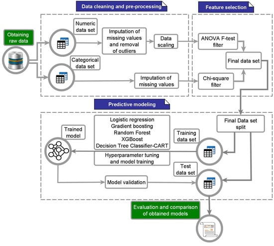
Figure 1.
Proposed methodology for modeling teacher job satisfaction.
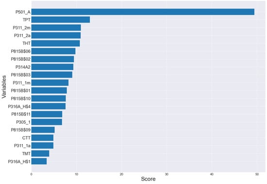
Figure 2.
ANOVA scores in predicting teacher job satisfaction.
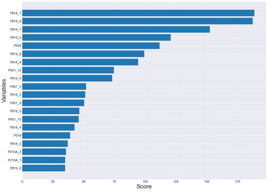
Figure 3.
Chi-Square scores in the prediction of teacher job satisfaction.
3.1. Data Cleaning and Preprocessing
We obtained the data set used for this study from the Encuesta Nacional a Docentes (ENDO) developed by the Peruvian Ministry of Education during 2018 [38]. The dimension of this data set is 15,087 instances and 942 attributes. The information contained in this survey is divided into the following categories: cemographics, housing and home; initial training; professional career and current job; health; economy; in-service training and education; media and information technologies; opinion and perception; and teaching practices. Table 1 shows a global summary of the data set generated by the function of the Data-Explorer package of the R language.

Table 1.
Overall summary of ENDO-2018 data set.
Of the 942 columns, we made a first manual selection of 407 variables belonging to the 9 categories mentioned above. The exclusion criteria were those columns with only one value for all the rows, as well as those with more than 40% of missing values, because these can cause errors or unexpected results, as suggested by the Ref. [39]. At this point it is important to clarify that some variables were empty due to the nature of the questions. For example, column P323 corresponding to the question: “If you could go back, would you choose to be a teacher again?” with alternatives of yes and no; answering yes to this question implied leaving column P324 empty corresponding to the question: Why would you not choose to be a teacher again, in order to move on to question 325. After this analysis, columns with at least 20% of missing data were filtered out, leaving 370 columns. It should be clarified that in this survey there were values with NEP code corresponding to the cells where the respondent did not specify the answer, so it was also necessary to input them.
In relation to the target variable, we constructed it from the answers to the question: All things considered, how satisfied are you with your job at this educational institution, which is found in the Opinion and Perception category of the survey in question.
3.1.1. Inputting Missing Values and Eliminating Outliers
In this task we proceeded to separate the data set into numerical with 40 columns and categorical 330 columns, then imputed by mode for the categorical variables. According to the Refs. [40,41] this procedure consists of filling in the missing data for each variable by mode when it is a categorical variable and by median for numerical variables. In relation to the numerical variables, it is important to clarify that this data set presented extreme values, so it was decided to impute the missing values by the median, because this measure is more representative and is not affected by the presence of these. These types of imputations in the statistical field are called simple imputation methods [42,43].
The Local Outlier Factor (LOF) algorithm identified 1785 instances as outliers in the numerical data set, and after identification these instances were removed in parallel in both data sets. For this algorithm the degree to which an object is extreme depends on the density of its local neighborhood, and it is possible to assign a LOF value to each object that would represent the probability that it is an extreme value [44]. For this technique we identified outliers as points with considerably lower density than their neighbors.
3.1.2. Robust Scaling Data
We applied this standardization method because it works with the median instead of the mean, as it is known that the median is more representative when there are some outliers. We calculated the median (50th percentile) and the 25th and 75th percentiles. Then, we subtracted the median from the values of each variable and divided it by the value of the interquartile range . The new values have a mean and median of zero and a standard deviation of 1 [39]. We show the equation we used in Appendix A.1.
3.2. Feature Selection
In this phase, we used the class of the Scikit-learn machine learning library. This implementation allowed the selection of the best features based on univariate statistical tests. According to the Ref. [45] this class allows the selection of the k features with the highest scores. To determine these scores, when input variables are numerical and the target variable is categorical it is possible to use the ANOVA F-statistic implemented in the function and when both are categorical we can use the Chi-square statistic implemented in the function of the library in the Ref. [39].
3.2.1. ANOVA F-Test Filter
For the selection of characteristics by this filter, we set up parameters and k = in class , giving as input the numerical data set and the teacher job satisfaction as the target variable. This configuration made it possible to obtain the scores shown in Figure 2. In addition, we shown the equations we used in Appendix A.2.
3.2.2. Chi-Square Filter
To use this filter we used the class of the aforementioned library, with the parameters and k = . To use this filter, first the ordinal coding of the categorical attributes was performed [46]. We detail this coding below. We calculated the score, returned by the mentioned function, using Equation (1) which corresponds to Pearson’s Chi-square statistic [47]. Pearson’s Chi-square statistic is a test of independence between two categorical variables [39].
are the observed values. are the expected values.
The scores obtained by this statistic are shown in Figure 3.
3.2.3. Construction of the Final Data Set
We constructed the final data by analyzing the relationship between the number of features and the accuracy gain in a logistic regression model, with a stratified cross-validation with 10 folds and 3 replicates. First, we applied this procedure to the categorical data set with the filter; then, on the numerical data set with the filter. In Figure 4, we showed that the gain margin in accuracy for the model is not significant as the number of features increases, so we chose nine features from the categorical data set and one from the numerical data set.
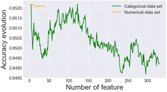
Figure 4.
Evolution of accuracy and number of features.
In Table 2, we show the description of the selected features and the respective naming in the ENDO-2018 data set.
Table 2.
Description of selected characteristics.
Of this final data set, variable is of nominal type, is of continuous numeric type, and the rest are of ordinal type.
Finally, we encoded the nominal variables with the .. module and the ordinal variables with the module, as described in the official manual [45] and the study presented by the Ref. [48]. The coding transforms a variable with n observations and k categories into k binary variables with n observations each [49,50]. coding, on the other hand, assigns an integer to each category, provided that the number of existing categories is known. In this case, no new column is added to the data, however it implies an order for the variable [49]. Table 3 shows the structure of the final data set. The variable Job Satisfaction constitutes our target variable, where one represents dissatisfied and zero represents satisfied.
Table 3.
Statistical summary of metrics in the training data set.
3.3. Predictive Modeling
3.3.1. Training and Test Data Set
We performed this task partitioning the data set into 70% for training and 30% for model validation, as [51,52] performed. We obtained 9911 instances to train and 3991 instances to validate as result of this partition.
After partitioning the data set, we verified the distribution of the classes in the target variable of the training data set, we show this distribution in Figure 5a, where we can see that this variable is partially unbalanced. According to the Refs. [53,54] unbalanced data can affect the result of the classification models, as they tend to bias the results towards the majority class. We solved this problem performing data balancing to the training data set, using the oversampling technique that consists of adding data to the minority class until we achieved a balance in both classes. Figure 5b shows the distribution of the classes after balancing the data.
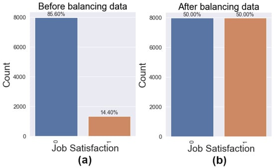
Figure 5.
Class distribution in the target variable. (a) Before data balancing. (b) After data balancing.
3.3.2. Hyper-Parameter Tuning and Model Training
To model training we used the Logistic Regression, Gradient Boosting, Random Forest, XG- Boost, Decision Trees-CART algorithms. To train the model, we considered optimal values that we calculated from a hyper-parameter tuning.
We tuned the hyper-parameters using the technique called Grid Search (GS), which is a widely used method to explore the configuration space of hyper-parameters in the field of machine learning [55,56]. GS performs an exhaustive search for the optimal configuration for a fixed domain of hyper-parameters, i.e. it trains a machine learning model with each combination of possible hyper-parameter values and then performs performance evaluation on the cross validation test data set of according to a previously defined metric [57]. In this study we used the sklearn GridSearchCV class, the area under the ROC curve score for classifier evaluation, and a cross-validation with k = 10. The main hyper-parameters for each model were taken from the list recommended by the Refs. [56,58]). The names, range of values, description, default values and optimal values of each one of the hyperameters that we use for each model are in Table 4.
Table 4.
Hyper-parameter settings.
3.3.3. Model Validation
We performed model validation on the test data set. We obtained the results of the present study from this task.
3.3.4. Evaluation and Comparison of Models Obtained
At this point we had to calculate the metrics of accuracy, sensitivity, specificity, area under the ROC curve (AUC), positive predictive value, negative predictive value. However, because the distribution of classes in the target variable is not balanced, we selected the best model based on sensitivity, area under the ROC curve (AUC), lower number of false-negatives and higher number of true-positives that we obtained from the confusion matrix. We show the structure of the confusion matrix for two classes in Figure 6.
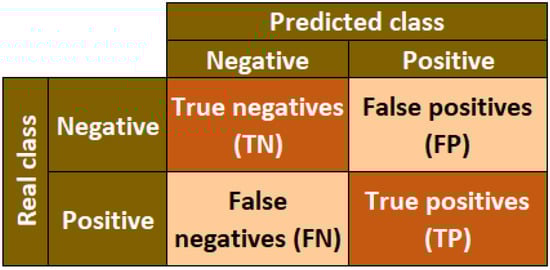
Figure 6.
Structure of a confusion matrix for two classes.
In Appendix A.3, we detailed the metrics for the confusion matrix.
4. Results
We made our experiments with the free Python machine learning library scikit-learn [45]. We trained and validated our models in a computer with these characteristics: AMD A12-9700P RADEON R7, 10 COMPUTE CORES 4C+6G at 2.50 GHz, 12 GB RAM, Windows 10 Home 64-bit operating system and x64 processor.
We evaluated the performance of five machine learning algorithms in the prediction of job satisfaction of basic education teachers in Peru. These algorithms are: Decision Trees-CART, Gradient Boosting, Logistic Regression, Random Forest and XGBoost.
In the Table 5 we show the main metrics that we obtained in the training stage with the hyper-parameter values presented in the previous section in combination with the K-Fold Cross-Validation technique with . Here it can be seen that the Random Forest model obtained the best results in 6 of the 8 metrics evaluated. These values are: mean accuracy of 0.77, mean sensitivity of 0.81, mean negative predictive value of 0.79, mean F1 score of 0.78, mean area under the ROC curve of 0.85, and a mean Cohen’s Kappa Coefficient of 0.53.
Table 5.
Statistical summary of metrics in the training data set.
In Table 6, we observe the results of applying the ANOVA test to the Cohen’s Kappa metric that we obtained after applying the K-Fold Cross-Validation technique with k = 100 in the training stage. The calculated F value = 11.489; p-value < 0.05, shows us that there are significant differences between the models analyzed.
Table 6.
ANOVA test in Cohen’s Kappa metric.
In Table 7, we show the results of Duncan’s test for comparison of means with Cohen’s Kappa metric. Here we find that group 4 is made up of the XGBoost and Random Forest models, this shows that in the training stage these algorithms have better performance in predicting job satisfaction of basic education teachers. We also show that the lowest value of the Logistic Regression algorithm with a mean value of Cohen’s Kappa of 0.4727280 is in group 1.
Table 7.
Duncan’s test on Cohe’s Kappa metric.
Figure 7 shows the confusion matrix of the models studied for the test data set. The confusion matrix of the Random Forest (c) and XGBoost (e) models show the lowest values of false-negatives 168 (dissatisfied teachers that the model classified as satisfied teachers), the highest values of true-positives 479 (dissatisfied teachers that the model classified as dissatisfied).
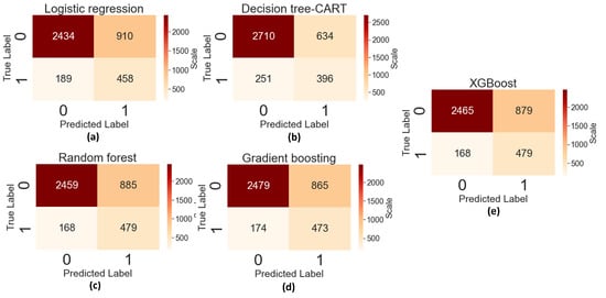
Figure 7.
Confusion matrix of the studied models. (a) Logistic regression. (b) Decision tree-CART. (c) Random forest. (d) Gradient boosting. (e) XGBoost.
Regarding the value of true negatives (Class 0: satisfied teachers) the Decision Trees-CART algorithm obtained the best result with 2710 (satisfied teachers that were correctly classified as satisfied). The lowest value of false-positives 634 (satisfied teachers who were classified as dissatisfied) was also obtained with the same algorithm.
Figure 8 shows the metrics we obtained after predicting the test data set. We will consider these metrics for the selection of the best model in predicting the job satisfaction of basic education teachers. Note that we obtained very similar values of Cohen’s Kappa metric between the XGBoost, Gradient Boosting and Random Forest models close to 0.33. The lowest value in this metric of 0.30 was obtained by the Logistic Regression model. Although models such as XGBoost, Gradient Boosting and Random Forest are formed by an ensemble of trees or estimators, the experiments show that in this metric the Decision Trees-CART algorithm slightly outperforms the ensemble models with a value of 0.34. Values obtained in the kappa coefficient of 0.33 and 0.34 by the models indicate an acceptable agreement between the actual classification and the predicted classification [59,60].
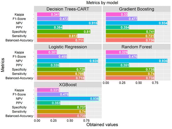
Figure 8.
Metrics obtained on the test data set.
With respect to the sensitivity metric, we obtained the best value with the Random Forest and XGBoost models of 0.74. In our problem domain, this value indicates the probability that the model correctly classifies a teacher belonging to the dissatisfied class [61]. The value obtained from this metric is very similar to that reported by the Ref. [17] in their “Review prognosis system to predict employees job satisfaction using deep neural network” they obtain a value of 0.75 for satisfied employees and 0.77 for dissatisfied employees. In the study entitled “A data mining based model for the prediction of satisfaction in the Surigao del Norte Division of the Department of Education” presented by the Ref. [27], they obtained a value of 0.72 for the k-nearest neighbors algorithm, in the case of the Naive Bayes algorithm a value of 0.74 and for the C4.5 algorithm a value of 0.80. It is important to clarify that these results were obtained for administrative employees and not for basic education teachers. To date, there are no studies that address the prediction of basic education teacher job satisfaction with the machine learning approach.
Since the test data set was not balanced, we decided to use the balanced accuracy metric, which is ideal for evaluating the performance of machine learning models on data sets with these characteristics [62,63,64]. In Figure 8, we can observe that the XGBoost, Random Forest and Gradient Boosting models obtain values close to 0.74, being the highest in the analyzed models. The value of this metric is similar to the results reported by the Ref. [18] where the authors compare job satisfaction prediction models for construction workers, with the CART and Neural Network algorithms, obtaining a value of 0.76 with the algorithm. of Decision Tress-CART. In the study in reference, the researchers used a data set of 280 instances with 20 independent variables. The feature selection technique for categorical variables used by the aforementioned authors is the same as that used in our study.
We obtained similar values of F1-Score = 0.48 with XGBoost, Gradient Boosting, and Random Forest. Decision Trees-CART obtained a very close value of 0.47.
Also note in Figure 8 that the highest value of the metric called negative predictive value (NPV) was 0.94 and we obtained it with the Random Forest and XGBoost algorithms.
Finally, Figure 8 also shows that Decision Trees-CART obtained a specificity value of 0.81, this suggests that this algorithm is adequate to predict class 0; that is, the satisfied teachers. Another metric, in the context of our study, that allows us to know the probability that the teacher is dissatisfied given that he was classified as such, is the positive predictive value. This value was also higher in the model built by the Decision Trees–CART algorithm. The positive predictive value was 0.38 in the model built by the Decision Trees–CART algorithm.
Figure 9 shows the area under the ROC curve that we have obtained after the prediction on the test data set. The models built with the Gradient Boosting and XGBoost algorithms obtain a value of AUC = 0.83, very close to this value is the Random Forest model with AUC = 0.82. With this, we demonstrate that the discriminant capacity of these models for the dissatisfied and satisfied class is good, as stated by the Ref. [65].
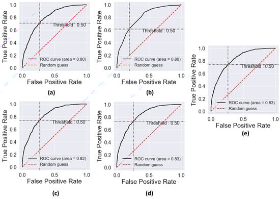
Figure 9.
Area under the ROC curve. (a) Logistic Regression model. (b) Decision Tree-CART model. (c) Random Forest model. (d) Gradient Boosting model. (e) XGBoost model.
It is important to note that in the feature selection process, as shown in Figure 2 and Figure 3 and Table 2, we found three variables which are: satisfaction of their relationship with the director, satisfaction with their life and satisfaction of their relationship with their colleagues that were reported by the Refs. [22,23,24] as variables that are significantly related to teacher job satisfaction. Our study confirms these findings.
Finally, in the educational sphere, our results provide new variables that could serve to better understand teacher job satisfaction. They also suggest that such variables should be considered when formulating teacher reassessment policies and reforms.
5. Conclusions
Our study identified and analyzed the most important and reliable predictors of job satisfaction of Peruvian basic education teachers based on data from the national survey of teachers ENDO-2018 prepared by the Ministry of Education of Peru. Since the original data set had numerical and categorical variables, it was necessary to carry out differentiated treatments, so we performed the selection of characteristics using the filter for the numerical variables and the filter for the categorical variables. The results show that the most important variables in the prediction are economic income, satisfaction with life, self-esteem, pedagogical activity, the relationship with the director, the perception of living conditions, with family relationships; health problems related to depression, and satisfaction with the relationship with peers. After evaluating and comparing the models built by the Logistic Regression, Decision Trees-CART, Random Forest, Gradient Boosting and XGBoost algorithms, our results show that in the test data set the XGBoost and Random Forest algorithms obtain similar results in 4 of the 8 metrics evaluated, where these are: balanced accuracy of 74%, sensitivity of 74%, F1-Score of 0.48, negative predictive value of 0.94. However, in terms of the area under the ROC curve, the XGBoost algorithm obtained 0.83, while Random Forest obtained 0.82. These algorithms also obtained the highest true-positive values (479 instances) and lowest false-negative values (168 instances) in the confusion matrix.
We hope the results of our study will serve as a starting point for the development of increasingly optimal predictive models of teacher job satisfaction classification, using other more sophisticated algorithms such as artificial neural networks.
Author Contributions
L.A.H.-A., M.S.A.-N. and J.M.B.-A. Conceptualization; L.A.H.-A., E.E.C.-V., J.M.-R., M.S.A.-N. and J.M.B.-A. Data Curation; L.A.H.-A., E.E.C.-V., H.D.C.-V., J.M.-R., M.S.A.-N., J.M.B.-A., M.Q.-L., R.H.-P. and M.V.-C. Formal analysis; L.A.H.-A. and Investigation; L.A.H.-A., J.M.-R., M.Q.-L., R.H.-P. and M.V.-C. Methodology; L.A.H.-A. Sofware; L.A.H.-A., H.D.C.-V., N.J.U.-G., M.Q.-L. and R.H.-P. Validation; L.A.H.-A., M.S.A.-N., J.M.B.-A., M.Q.-L. and R.H.-P. Writing—original draft; L.A.H.-A., J.M.-R. and M.V.-C. Writing—review & editing. All authors have read and agreed to the published version of the manuscript.
Funding
This research received no external funding.
Data Availability Statement
Data availability. The data set analyzed during the current study and that support the findings of this study are available in: https://doi.org/10.17632/b7wbthz6hs.2 (accessed on 30 January 2023). The source code is available at: https://github.com/luisholgado/teacher_job_satisfaction/blob/main/teacher_job_satisfaction_code.ipynb (accessed on 2 March 2023).
Conflicts of Interest
The authors declare no conflict of interest.
Appendix A
Appendix A.1
The Equation (A1) formally shows this type of data scaling.
where, and are the 75th and 25th percentiles respectively.
The implementation of this scaling method is found in the class of the sklearn pre-processing module.
Appendix A.2
The F statistic allows to obtain these scores, which we can see in Equation (A2).
= Sum of squares between groups:
= Sum of squares within groups:
In addition, , , m is the number of levels of our target variable and n is the number of observations, is the mean in group j, is the total mean [66].
Appendix A.3
Balanced accuracy For binary classification this value is equal to the arithmetic mean of the sensitivity and specificity.
- are the true-positives. are the true negatives.
- are the false-negatives. are the false-positives.
Sensitivity Represents the proportion of true-positives that the model predicted correctly (Positive Class 1: Dissatisfied).
Specificity Represents the proportion of true negatives that the model predicted correctly (Negative Class 0: Satisfactory).
Positive predictive value (PPV) Also called precision, represents the probability of an instance being of the positive class having been predicted as positive by the model.
Negative predictive value (NPV) Represents the probability of an instance being of the negative class having been predicted as negative by the model.
Cohen’s kappa coefficient Measures the agreement between classifiers.
- where, : the percentage of agreement observed.
- : is the probability that the inter-rater agreement is due to chance.
Area under the ROC curve (AUC). Indicates how good the model is at discriminating instances of the positive class and the negative class. This value fluctuates between 0 and 1. According to the Ref. [67], the closer this value is to 1, the greater the discriminating capacity of the model.
Appendix A.4
Table A1.
Data dictionary of the features selected with the ANOVA F-test filter.
Table A1.
Data dictionary of the features selected with the ANOVA F-test filter.
| Description | Variable |
|---|---|
| Total income in the previous month | P311_2m |
| Time since first job as a teacher | TPT |
| Number of months you have been working at this school as a contract | P311_2m |
| Number of years you have been working consecutively at this school as a contract | P311_2a |
| Travel time in hours to work | THT |
| Number of times you attended services or performances of film features in the past 12 months | P815B$06 |
| Number of times you visited monuments in the last 12 months | P815B$02 |
| Average number of students per classroom | P314A2 |
| Number of times you visited archaeological sites in the last 12 months | P815B$03 |
| Number of months you have been working at this school as appointed | P311_1m |
| Number of times you visited museums in the last 12 months | P815B$01 |
| Number of times you visited book fairs in the last 12 months | P815B$10 |
| Amount of time spent working as a team or conversing with colleagues from your school | P316A_H$4 |
| Number of times you visited craft fairs in the last 12 months | P815B$11 |
| Number of public schools in which you currently teach | P305_1 |
| Number of times you visited libraries or reading rooms in the last 12 months | P815B$09 |
| Total cost of commuting to work | CTT |
| Number of years you have worked consecutively at this school as appointed | P311_1a |
| Commute time in minutes to work | TMT |
| Time spent teaching classes in a typical week | P316A_H$1 |
Table A2.
Data dictionary of the features selected with the Chi-Square filter.
Table A2.
Data dictionary of the features selected with the Chi-Square filter.
| Description | Variable |
|---|---|
| Satisfaction with your life | P818_1 |
| Satisfaction with your self-esteem | P818_6 |
| Satisfaction with your pedagogical activity | P819_1 |
| Satisfaction with the relationship with the director | P819_5 |
| Perception of living conditions | P509 |
| Satisfaction with your salary | P819_8 |
| Satisfaction with their family relationships | P818_8 |
| The year before she suffered from depression | P401_12 |
| Satisfaction with the relationship with their colleagues | P819_4 |
| Frequency with which you work with poor lighting in class | P407_3 |
| Satisfaction with the achievements of their students | P819_2 |
| The previous year he suffered stress | P401_9 |
| Satisfaction with the conditions of your future retirement | P818_5 |
| The previous year he suffered anxiety | P401_10 |
| Satisfaction with education that you can give your children | P818_4 |
| If you could choose any teaching position in the country, would it be in the same district? | P319 |
| Satisfaction with your health | P818_2 |
| Qualification of the teaching methodology used by teachers in their teacher training | P210A_2 |
| Qualification of the thematic contents of the courses/learning areas received in their teacher training | P210A_1 |
| Satisfaction with their relationship with parents | P819_6 |
References
- Hassan, O.; Ibourk, A. Burnout, self-efficacy and job satisfaction among primary school teachers in Morocco. Soc. Sci. Humanit. Open 2021, 4, 100148. [Google Scholar] [CrossRef]
- Serrano-García, V.; Ortega-Andeane, P.; Reyes-Lagunes, I.; Riveros-Rosas, A. Traducción y Adaptación al Español del Cuestionario de Satisfacción Laboral para Profesores. Acta Investig. Psicol. 2015, 5, 2112–2123. [Google Scholar] [CrossRef]
- Lopes, J.; Oliveira, C. Teacher and school determinants of teacher job satisfaction: A multilevel analysis. Sch. Eff. Sch. Improv. 2020, 31, 641–659. [Google Scholar] [CrossRef]
- Sadeghi, K.; Ghaderi, F.; Abdollahpour, Z. Self-reported teaching effectiveness and job satisfaction among teachers: The role of subject matter and other demographic variables. Heliyon 2021, 7, e07193. [Google Scholar] [CrossRef]
- Aouadni, I.; Rebai, A. Decision support system based on genetic algorithm and multi-criteria satisfaction analysis (MUSA) method for measuring job satisfaction. Ann. Oper. Res. 2016, 256, 3–20. [Google Scholar] [CrossRef]
- Lee, A.N.; Nie, Y. Understanding teacher empowerment: Teachers’ perceptions of principal’s and immediate supervisor’s empowering behaviours, psychological empowerment and work-related outcomes. Teach. Teach. Educ. 2014, 41, 67–79. [Google Scholar] [CrossRef]
- Valles-Coral, M.A.; Salazar-Ramírez, L.; Injante, R.; Hernandez-Torres, E.A.; Juárez-Díaz, J.; Navarro-Cabrera, J.R.; Pinedo, L.; Vidaurre-Rojas, P. Density-Based Unsupervised Learning Algorithm to Categorize College Students into Dropout Risk Levels. Data 2022, 7, 165. [Google Scholar] [CrossRef]
- Lopes Martins, D. Data science teaching and learning models: Focus on the Information Science area. Adv. Notes Inf. Sci. 2022, 2, 140–148. [Google Scholar] [CrossRef]
- Araoz, E.G.E.; Ramos, N.A.G. Satisfacción laboral y compromiso organizacional en docentes de la amazonía peruana. Educ. Form. 2021, 6, e3854. [Google Scholar] [CrossRef]
- Ruiz-Quiles, M.; Moreno-Murcia, J.A.; Vera-Lacárcel, J.A. Del soporte de autonomía y la motivación autodeterminada a la satisfacción docente. Eur. J. Educ. Psychol. 2015, 8, 68–75. [Google Scholar] [CrossRef]
- Gabrani, G.; Kwatra, A. Machine learning based predictive model for risk assessment of employee attrition. Lect. Notes Comput. Sci. Incl. Subser. Lect. Notes Artif. Intell. Lect. Notes Bioinform. 2018, 10963 LNCS, 189–201. [Google Scholar] [CrossRef]
- Sisodia, D.S.; Vishwakarma, S.; Pujahari, A. Evaluation of machine learning models for employee churn prediction. In Proceedings of the International Conference on Inventive Computing and Informatics, ICICI 2017, Coimbatore, India, 23–24 November 2017; pp. 1016–1020. [Google Scholar] [CrossRef]
- Yogesh, I.; Suresh Kumar, K.R.; Candrashekaran, N.; Reddy, D.; Sampath, H. Predicting Job Satisfaction and Employee Turnover Using Machine Learning. J. Comput. Theor. Nanosci. 2020, 17, 4092–4097. [Google Scholar] [CrossRef]
- Homocianu, D.; Plopeanu, A.P.; Florea, N.; Andries, A.M. Exploring the patterns of job satisfaction for individuals aged 50 and over from three historical regions of Romania. An inductive approach with respect to triangulation, cross-validation and support for replication of results. Appl. Sci. 2020, 10, 2573. [Google Scholar] [CrossRef]
- Saisanthiya, D.; Gayathri, V.M.; Supraja, P. Employee attrition prediction using machine learning and sentiment analysis. Int. J. Adv. Trends Comput. Sci. Eng. 2020, 9, 7550–7557. [Google Scholar] [CrossRef]
- Seok, B.W.; Wee, K.H.; Park, J.Y.; Anil Kumar, D.; Reddy, N.S. Modeling the teacher job satisfaction by artificial neural networks. Soft Comput. 2021, 25, 11803–11815. [Google Scholar] [CrossRef]
- Rustam, F.; Ashraf, I.; Shafique, R.; Mehmood, A.; Ullah, S.; Sang Choi, G. Review prognosis system to predict employees job satisfaction using deep neural network. Comput. Intell. 2021, 37, 924–950. [Google Scholar] [CrossRef]
- Chen, T.; Cao, Z.; Cao, Y. Comparison of job satisfaction prediction models for construction workers: Cart vs. neural network. Teh. Vjesn. 2021, 28, 1174–1181. [Google Scholar] [CrossRef]
- Hong-Hua, M.; Mi, W.; Hong-Yum, L.; Yong-Mei, H. Influential factors of China’s elementary school teachers’ job satisfaction. Springer Proc. Math. Stat. 2016, 167, 339–361. [Google Scholar] [CrossRef]
- Tomás, J.M.; De Los Santos, S.; Fernández, I. Job satisfaction of the Dominican teacher: Labor background. Rev. Colomb. Psicol. 2019, 28, 63–76. [Google Scholar] [CrossRef]
- Asadujjaman, M.D.; Rashid, M.H.O.; Nayon, M.A.A.; Biswas, T.K.; Arani, M.; Billal, M.M. Teachers’ job satisfaction at tertiary education: A case of an engineering university in Bangladesh. In Proceedings of the International Conference on e-Learning, ICEL, Sakheer, Bahrain, 6–7 December 2020; pp. 238–242. [Google Scholar] [CrossRef]
- Al-Mahdy, Y.F.H.; Alazmi, A.A. Principal Support and Teacher Turnover Intention in Kuwait: Implications for Policymakers. Leadersh. Policy Sch. 2023, 22, 44–59. [Google Scholar] [CrossRef]
- Luque-Reca, O.; García-Martínez, I.; Pulido-Martos, M.; Lorenzo Burguera, J.; Augusto-Landa, J.M. Teachers’ life satisfaction: A structural equation model analyzing the role of trait emotion regulation, intrinsic job satisfaction and affect. Teach. Teach. Educ. 2022, 113, 103668. [Google Scholar] [CrossRef]
- Eirín-Nemiña, R.; Sanmiguel-Rodríguez, A.; Rodríguez-Rodríguez, J. Professional satisfaction of physical education teachers. Sport Educ. Soc. 2022, 27, 85–98. [Google Scholar] [CrossRef]
- Karunanayake, V.J.; Wanniarachchi, J.C.; Karunanayake, P.N.; Rajapaksha, U.U. Intelligent System to Verify the Effectiveness of Proposed Teacher Transfers Incorporating Human Factors. In Proceedings of the ICARC 2022—2nd International Conference on Advanced Research in Computing: Towards a Digitally Empowered Society, Belihuloya, Sri Lanka, 23–24 February 2022; pp. 1–6. [Google Scholar] [CrossRef]
- Saleh, L.; Abu-Soud, S. Predicting Jordanian Job Satisfaction Using Artificial Neural Network and Decision Tree. In Proceedings of the 2021 11th International Conference on Advanced Computer Information Technologies, ACIT 2021—Proceedings, Deggendorf, Germany, 15–17 September 2021; pp. 735–738. [Google Scholar] [CrossRef]
- Talingting, R.E. A data mining-driven model for job satisfaction prediction of school administrators in DepEd Surigao del Norte division. Int. J. Adv. Trends Comput. Sci. Eng. 2019, 8, 556–560. [Google Scholar] [CrossRef]
- Arambepola, N.; Munasinghe, L. What makes job satisfaction in the information technology industry? In Proceedings of the 2021 International Research Conference on Smart Computing and Systems Engineering (SCSE), Colombo, Sri Lanka, 16 September 2021; pp. 99–105. [Google Scholar] [CrossRef]
- Lu, M.H.; Luo, J.; Chen, W.; Wang, M.C. The influence of job satisfaction on the relationship between professional identity and burnout: A study of student teachers in Western China. Curr. Psychol. 2022, 41, 289–297. [Google Scholar] [CrossRef]
- Perera, H.N.; Maghsoudlou, A.; Miller, C.J.; McIlveen, P.; Barber, D.; Part, R.; Reyes, A.L. Relations of science teaching self-efficacy with instructional practices, student achievement and support, and teacher job satisfaction. Contemp. Educ. Psychol. 2022, 69, 102041. [Google Scholar] [CrossRef]
- Zhang, J.; Yin, H.; Wang, T. Exploring the effects of professional learning communities on teacher’s self-efficacy and job satisfaction in Shanghai, China. Educ. Stud. 2023, 49, 17–34. [Google Scholar] [CrossRef]
- Xia, J.; Wang, M.; Zhang, S. School culture and teacher job satisfaction in early childhood education in China: The mediating role of teaching autonomy. Asia Pac. Educ. Rev. 2022, 24, 101–111. [Google Scholar] [CrossRef]
- Zhang, X.; Cheng, X.; Wang, Y. How Is Science Teacher Job Satisfaction Influenced by Their Professional Collaboration? Evidence from Pisa 2015 Data. Int. J. Environ. Res. Public Health 2023, 20, 1137. [Google Scholar] [CrossRef]
- Aktan, O.; Toraman, Ç. The relationship between Technostress levels and job satisfaction of Teachers within the COVID-19 period. Educ. Inf. Technol. 2022, 27, 10429–10453. [Google Scholar] [CrossRef] [PubMed]
- Elrayah, M. Improving Teaching Professionals’ Satisfaction through the Development of Self-efficacy, Engagement, and Stress Control: A Cross-sectional Study. Educ. Sci. Theory Pract. 2022, 22, 1–12. [Google Scholar]
- Smet, M. Professional development and teacher job satisfaction: Evidence from a multilevel model. Mathematics 2022, 10, 51. [Google Scholar] [CrossRef]
- Hussain, S.; Saba, N.U.; Ali, Z.; Hussain, H.; Hussain, A.; Khan, A. Job Satisfaction as a Predictor of Wellbeing Among Secondary School Teachers. SAGE Open 2022, 12, 21582440221138726. [Google Scholar] [CrossRef]
- MINEDU. Ministerio de Educación del Perú|MINEDU. 2021. Available online: https://escale.minedu.gob.pe/uee/-/document_library_display/GMv7/view/5384052 (accessed on 30 September 2022).
- Brownlee, J.; Sanderson, M.; Koshy, A.; Cheremskoy, A.; Halfyard, J. Machine Learning Mastery With Python: Data Cleaning, Feature Selection, and Data Transforms in Python; Machine Learning Mastery: Vermont, VIC, Australia, 2020. [Google Scholar]
- Useche, L.; Mesa, D. Una introducción a la imputación de valores perdidos. Terra 2006, XXII, 127–152. [Google Scholar]
- Navarro-Pastor, J.; Losilla-Vidal, J. Psicothema—Análisis De Datos Faltantes Mediante Redes Neuronales Artificiales. Psicothema 2000, 12, 503–510. [Google Scholar]
- Cuesta, M.; Fonseca-Pedrero, E.; Vallejo, G.; Muñiz, J. Datos perdidos y propiedades psicométricas en los tests de personalidad. An. Psicol. 2013, 29, 285–292. [Google Scholar] [CrossRef]
- Rosati, G. Construcción de un modelo de imputación para variables de ingreso con valores perdidos a partir de ensamble learning: Aplicación en la Encuesta permanente de hogares (EPH). SaberEs 2017, 9, 91–111. [Google Scholar] [CrossRef]
- Alshawabkeh, M.; Jang, B.; Kaeli, D. Accelerating the local outlier factor algorithm on a GPU for intrusion detection systems. In Proceedings of the International Conference on Architectural Support for Programming Languages and Operating Systems—ASPLOS, Pittsburgh, PA, USA, 14 March 2010; pp. 104–110. [Google Scholar] [CrossRef]
- Pedregosa, F.; Varoquaux, G.; Gramfort, A.; Michel, V.; Thirion, B.; Grisel, O.; Blondel, M.; Prettenhofer, P.; Weiss, R.; Dubourg, V.; et al. Scikit-learn: Machine Learning in Python. J. Mach. Learn. Res. 2011, 12, 2825–2830. [Google Scholar]
- Dashdondov, K.; Lee, S.M.; Kim, M.H. OrdinalEncoder and PCA based NB Classification for Leaked Natural Gas Prediction Using IoT based Remote Monitoring System. Smart Innov. Syst. Technol. 2021, 212, 252–259. [Google Scholar] [CrossRef]
- Quintero, M.A.; Duran, M. Análisis del error tipo I en las pruebas de bondad de ajuste e independencia utilizando el muestreo con parcelas de tamaño variable (Bitterlich). Bosque 2004, 25, 45–55. [Google Scholar] [CrossRef]
- Hancock, J.T.; Khoshgoftaar, T.M. Survey on categorical data for neural networks. J. Big Data 2020, 7, 1–41. [Google Scholar] [CrossRef]
- Potdar, K. A Comparative Study of Categorical Variable Encoding Techniques for Neural Network Classifiers. Int. J. Comput. Appl. 2017, 175, 975–8887. [Google Scholar] [CrossRef]
- Zheng, A.; Casari, A. Feature Engineering for Machine Learning: Principles and Techniques for Data Scientists, 1st ed.; O’Reilly Media, Inc.: Sebastopol, Russia, 2018; p. 218. [Google Scholar]
- Fallucchi, F.; Coladangelo, M.; Giuliano, R.; De Luca, E.W. Predicting employee attrition using machine learning techniques. Computers 2020, 9, 86. [Google Scholar] [CrossRef]
- Moon, N.N.; Mariam, A.; Sharmin, S.; Islam, M.M.; Nur, F.N.; Debnath, N. Machine learning approach to predict the depression in job sectors in Bangladesh. Curr. Res. Behav. Sci. 2021, 2, 100058. [Google Scholar] [CrossRef]
- Torres-Vásquez, M.; Hernández-Torruco, J.; Hernández-Ocaña, B.; Chávez-Bosquez, O.; Torres-Vásquez, M.; Hernández-Torruco, J.; Hernández-Ocaña, B.; Chávez-Bosquez, O. Impacto de los algoritmos de sobremuestreo en la clasificación de subtipos principales del síndrome de guillain-barré. Ingenius. Rev. Cienc. Tecnol. 2021, 25, 20–31. [Google Scholar] [CrossRef]
- Bourel, M.; Segura, A.M.; Crisci, C.; López, G.; Sampognaro, L.; Vidal, V.; Kruk, C.; Piccini, C.; Perera, G. Machine learning methods for imbalanced data set for prediction of faecal contamination in beach waters. Water Res. 2021, 202, 117450. [Google Scholar] [CrossRef]
- Elgeldawi, E.; Sayed, A.; Galal, A.R.; Zaki, A.M. Hyper-parameter Tuning for Machine Learning Algorithms Used for Arabic Sentiment Analysis. Informatics 2021, 8, 79. [Google Scholar] [CrossRef]
- Yang, L.; Shami, A. On hyper-parameter optimization of machine learning algorithms: Theory and practice. Neurocomputing 2020, 415, 295–316. [Google Scholar] [CrossRef]
- Wu, J.; Chen, X.Y.; Zhang, H.; Xiong, L.D.; Lei, H.; Deng, S.H. Hyper-parameter Optimization for Machine Learning Models Based on Bayesian Optimization. J. Electron. Sci. Technol. 2019, 17, 26–40. [Google Scholar] [CrossRef]
- Buitinck, L.; Louppe, G.; Blondel, M.; Pedregosa, F.; Mueller, A.; Grisel, O.; Niculae, V.; Prettenhofer, P.; Gramfort, A.; Grobler, J.; et al. API design for machine learning software: Experiences from the scikit-learn project. In Proceedings of the ECML PKDD Workshop: Languages for Data Mining and Machine Learning, Würzburg, Germany, 16–20 September 2019; pp. 108–122. [Google Scholar]
- Wiȩckowska, B.; Kubiak, K.B.; Jóźwiak, P.; Moryson, W.; Stawińska-Witoszyńska, B. Cohen’s Kappa Coefficient as a Measure to Assess Classification Improvement following the Addition of a New Marker to a Regression Model. Int. J. Environ. Res. Public Health 2022, 19, 10213. [Google Scholar] [CrossRef]
- Fujimura, S.; Kojima, T.; Okanoue, Y.; Shoji, K.; Inoue, M.; Omori, K.; Hori, R. Classification of Voice Disorders Using a One-Dimensional Convolutional Neural Network. J. Voice 2022, 36, 15–20. [Google Scholar] [CrossRef] [PubMed]
- Kim, K.B.; Park, H.J.; Song, D.H. Combining Supervised and Unsupervised Fuzzy Learning Algorithms for Robust Diabetes Diagnosis. Appl. Sci. 2022, 13, 351. [Google Scholar] [CrossRef]
- Kvak, D.; Chromcová, A.; Biroš, M.; Hrubý, R.; Kvaková, K.; Pajdaković, M.; Ovesná, P. Chest X-ray Abnormality Detection by Using Artificial Intelligence: A Single-Site Retrospective Study of Deep Learning Model Performance. BioMedInformatics 2023, 3, 82–101. [Google Scholar] [CrossRef]
- Makansi, F.; Schmitz, K.; Makansi, F.; Schmitz, K. Data-Driven Condition Monitoring of a Hydraulic Press Using Supervised Learning and Neural Networks. Energies 2022, 15, 6217. [Google Scholar] [CrossRef]
- Moreno-Ibarra, M.A.; Villuendas-Rey, Y.; Lytras, M.D.; Yáñez-Márquez, C.; Salgado-Ramírez, J.C. Classification of Diseases Using Machine Learning Algorithms: A Comparative Study. Mathematics 2021, 9, 1817. [Google Scholar] [CrossRef]
- Gironés, J.; Casas, J.; Minguillón, J.; Caihuelas, R. Minería De Datos: Modelos y Algoritmos, 1st ed.; Editorial UOC: Barcelona, Spain, 2017; p. 274. [Google Scholar]
- Montgomery, D. Diseño y Análisis De Experimentos, 2nd ed.; Limusa Wiley: México City, Mexico, 2004; pp. 69–71. [Google Scholar]
- Cerda, J.; Cifuentes, L. Uso de curvas ROC en investigación clínica: Aspectos teórico-prácticos. Rev. Chil. Infectol. 2012, 29, 138–141. [Google Scholar] [CrossRef]
Disclaimer/Publisher’s Note: The statements, opinions and data contained in all publications are solely those of the individual author(s) and contributor(s) and not of MDPI and/or the editor(s). MDPI and/or the editor(s) disclaim responsibility for any injury to people or property resulting from any ideas, methods, instructions or products referred to in the content. |
© 2023 by the authors. Licensee MDPI, Basel, Switzerland. This article is an open access article distributed under the terms and conditions of the Creative Commons Attribution (CC BY) license (https://creativecommons.org/licenses/by/4.0/).