Featured Application
Tooth score morphology characterization through the use of landmarks and semilandmarks may be used to discern which species or carnivore groups modified bone assemblages.
Abstract
Taphonomic studies aim to identify the modifying agents that intervene in bone assemblages found at archaeopaleontological sites. Carnivores may modify, accumulate, or scavenge skeletal parts inflicting tooth marks, including scores, on the cortical surface. Several works have studied tooth score morphology to discern which carnivore group modified the bone assemblages, achieving different results. In the present study, different methods based on the use of landmarks and semilandmarks have been tested to describe and analyze the score profile cross-sections of spotted and brown hyenas, leopards, and lions. According to our results, the already published seven-landmark method is useful in order to differentiate between carnivore species from different families (e.g., felids and hyenids). Meanwhile, felid species (e.g., leopards and lions) cannot be consistently distinguished using any of the methods tested here. In contrast, hyenid species can be morphologically differentiated. On the other hand, the use of semilandmarks does not generally improve morphological characterization and distinction, but low numbers of landmarks and the inclusion of the score’s deepest point might provide the best results when semi-automatic semilandmark models are preferred to avoid sampling biases.
1. Introduction
Carnivore action on bone assemblages is difficult to differentiate due to equifinality. Different carnivore species may produce similar bone damage, impeding, in some cases, an accurate taxonomic characterization of the taphonomic agents intervening in archaeopaleontological sites. Furthermore, archaeopaleontological sites are usually described as palimpsests, which implies that several taphonomic agents (e.g., humans, carnivores, etc.) may have modified those bone assemblages. A suitable description of the taphonomic agents involved in the bone modification of archaeopaleontological sites is crucial to formulating hypotheses on hominin-carnivore interactions, hominin subsistence patterns, or site formation processes [1,2,3,4,5,6,7]. On this basis, much neotaphonomic research has been conducted in order to find variables that would not only allow the identification of modifying agents in the fossil record (i.e., humans or carnivores), but also the specification of carnivore groups and taxa based on the bone surface modifications they generate [8,9,10,11].
For instance, tooth mark dimensions have been analysed by several authors to statistically differentiate the pits and scores produced by different carnivore species [12,13,14,15,16]. Pits have been described as circular depressions, while tooth scores are elongated marks characterized by U-shaped cross-sections [1,17]. Both width and length have been recorded on bones modified by different carnivores (e.g., felids, hyenids, canids, ursids, etc), while considering bone region (e.g., epiphysis versus long bone shaft). For instance, pit and score dimensions have been used to discuss the accumulating agent of bone assemblages from Olduvai Gorge (Tanzania) or Sima de los Huesos (Spain) [12,13,14]. The analyses of tooth mark dimensions from the FLK Zinj site (Olduvai Gorge, Tanzania) showed that both felids and hyenids modified the bone assemblage [12]. Cut and percussion marks produced by hominins were also recorded on the FLK Zinj bone assemblage [3,7]. According to the analyses and results obtained, it has been argued that hyenas were the last modifying agent of the ungulate carcasses from the FLK Zinj [12]. Thus, either hyenas may have scavenged ungulate carcasses that were first defleshed by hominins and felids, or hyenas may have just consumed the marrow of bones first scavenged by hominins after a primary consumption by felids [12]. These results imply that early hominins from Olduvai Gorge were not the first taphonomic agents in the consumption change [12]. Further research has demonstrated that carnivore body mass and the location of the tooth mark, i.e., on the epiphysis or diaphysis, determines tooth mark dimensions [15], so that tooth marks inflicted on long bone shafts by small and large carnivores are statistically differentiable [14,15,16]. However, both pit and score dimensions overlap among different carnivore taxa. That means that while carnivore size could be inferred from tooth mark dimensions, this same variable cannot be used to determine carnivore taxa. Thus, felid and hyenid species could not be differentiated. These results could not support the three-stage model hypothesis (carnivore-hominin-carnivore) for the FLK Zinj bone assemblage [14].
On the other hand, tooth mark frequency or the number of tooth marks inflicted by bone have been also explored in order to determine agency in bone assemblages, and thus, overcome the equifinality biases that tooth mark size could not totally solve. The extent of bone modification depends on the type of carnivore involved at the site. It has been argued that felids modify skeletal body parts less intensively than hyenas [2,12]. Further research showed that a low tooth mark frequency on long bone shafts may be produced by a primary access of felids to animal carcasses, or by a secondary hyenid access [18]. Thus, in multi-agent scenarios such as archaeopaleontological sites where several taphonomic agents may modify skeletal parts, tooth mark frequency also shows equifinality problems.
Recently, new methodological approaches combining geometric morphometric (GM) analyses and virtual reconstructions of tooth marks have improved carnivore taxa identification [19,20,21,22,23]. The examination of tooth mark morphology along with tooth mark dimensions showed promising results regarding the differentiation of carnivore groups. Despite the valuable methodological progress presented by Yravedra et al. [19], concerning the morphological registration and study of carnivore tooth scores, we believe that the lack of specificity regarding the selection of the score cross-section (most characteristic U-shape section within the 30–70% mark length) could cause biases during data collection, not only in relation to the observer’s own objectivity, but also to the potential intra-specific morphological variation along the score profile. Therefore, we consider it necessary to assess this method in a more detailed manner. For that purpose, in the present study, we evaluate the original, as well as novel landmark-based models, to explore felid and hyenid tooth score morphology at different points along the length of scores, with the aim of proposing some methodological recommendations for future research in this line.
2. Materials and Methods
2.1. Sample
The sample employed in the present study (Table 1) includes tooth scores generated by spotted (Crocuta crocuta) and brown hyenas (Parahyena brunnea), lions (Panthera leo), and leopards (Panthera pardus) (Figures S1–S4). The sample created by spotted hyenas [24] and lions [25] was collected from adult equid long bones consumed at the Cabárceno Nature Park in Cantabria (Spain), where carnivores live in captivity. The leopard and brown hyena sample stems from modern carnivore dens housed at the Ditsong Museum in Pretoria (see [26,27]) that were previously studied by Brain [2]. Preferably, tooth marks from ungulate long bone shafts were selected, although also a small amount of baboon long bones modified by leopards was included to increase sample size considering the lack of significant differences between the ungulate and baboon sample previously documented by Arriaza et al. [26].

Table 1.
Tooth score sample used in this study.
Tooth marks, including scores, were re-examined by at least one of the co-authors of the present study—either M.C.A. or J.A.—with the aid of a 20× hand lens. Then, conspicuous scores were selected for digitization according to their location on long bone shafts and their preservation. The 3D models were already generated for previous publications [19,26,27] using photogrammetric methods, as described in Yravedra et al. [19], that are capable of extracting information on the geometric properties of an object based on the capture of several images. Between 13 and 16 pictures were taken with the aid of a Canon EOS 700D reflex camera, with 60 mm macro lenses for each score, depending on the geometry of the bone and the shape of the mark. For image data capture, specimens were placed on a photographic table with the lighting adjusted to keep the bone permanently well illuminated next to a millimetric scale; the focus and brightness parameters were adjusted at the beginning of the process to remain constant; and a tripod was used to stabilize the camera during the entire process.
Once the photographs had been taken, they were processed using the photogrammetric reconstruction software GRAPHOS (inteGRAted PHOtogrammetric Suite) [28] to generate a 3D model for each mark. This software includes self-camera calibration, so it allows for the estimation of the internal camera parameters, including lens distortion. In particular, the Fraser calibration model [29] was used, which includes 12 parameters: focal length (f), principal point (x0, y0), principal point offsets (x1, y1), radial lens distortion (k1, k2, k3), and decentering distortion (p1, p2), scaling, and affinity factors. The generation of the precise metrical models of each score took 30–45 min depending on the final number of photos. Subsequently, the Global Mapper software was used to define and measure 2D cross-sectional mark profiles. Alongside cross-sections at the mid-length of each score, profiles at 65% and 35% were taken to assess the statements made by Yravedra et al. and Maté-González et al. [19,30] that sections between 30% and 70% of the mark length are equally representative and valid for morphometric studies. Additionally, cross-sectional profiles were also taken at the portion where the typical score U-shape was most conspicuous, as this section has been commonly selected for previous studies [19].
2.2. Methodology
2.2.1. Geometric Morphometrics
The GM tool kit was used to characterize and analyze the carnivore tooth scores on the basis of the extracted cross-sections. GM is a method based on the use of landmarks (homologous points across specimens) that contain morphological information in the form of Cartesian coordinates [31,32,33,34] and that enable the study of shape and form (shape and size) variance and co-variance [35,36,37]. While shape can be studied after standardization procedures that remove the effects in the orientation, location, and size of the elements under study, form requires the omission of the scaling step, so that size (or centroid size as it is commonly known in GM) can be considered alongside shape. In addition to landmarks, semilandmarks have been introduced in GM studies to register areas that lack clear homologous points [32,38], long curves, or surfaces. The use of semilandmarks has thus allowed the detailed quantification of 2D and 3D geometries. In order to be able to combine semilandmarks with fixed landmarks, semilandmarks need to be transformed into homologous points through the application of sliding algorithms [39] by ensuring the correspondence of the semilandmarks and the avoidance of arbitrary location. The process of sliding semilandmarks aims to minimize shape differences between each slid specimen (targets) and the template (usually a mean shape) through the repetitive sliding of all the semilandmarks at the same time. The application of this technique based on the Thin-Plate-Spline (TPS) formalism accounts for local shape deformation using a mathematical model that interpolates the space found between two sets of homologous landmarks as smoothly as possible [38].
Landmarking procedures were performed using an automated procedure programmed in the R programming language [40,41], while sliding was performed using functions from the geomorph R library [42]. First, 7 2D fixed landmarks were collected for each score cross-section following the guidelines established in Maté-González et al. [30] and Yravedra et al. [19] (Figure 1). Additionally, we tested the use of semilandmarks to characterize score cross-sections at 50% of the total length and at the most conspicuous U-shaped score profile by generating different models (Figure 1) that included; 10 (Figure 1b), 25 (Figure 1c), and 50 (Figure 1d) 2D semilandmarks slid along a single curve; and 10 (Figure 1e), 20 (Figure 1f), and 30 (Figure 1g) semilandmarks slid along 2 curves defined by the lateral limits on the score cross-section and its deepest point, meaning the latter models include three additional fixed landmarks. Landmarking was performed by two authors (M.C.A. and J.A.) in different sessions and interchanging the carnivore groups. This allowed the analysis of inter and intra-observer error, as in previous studies [20,22], by assessing the significance of the differences observed between the landmark configurations obtained from the same dataset, using multivariate analyses of variance (MANOVAs). The confirmation of the method replicability, based on the obtention of non-significant differences (p > 0.05) between the carnivore group means (e.g., the lion sample landmarked by M.C.A. versus the lion sample landmarked by J.A.), opened the way for the performance of the present study.
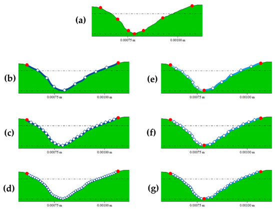
Figure 1.
Landmark and semilandmark models created for the present study on an example of a leopard score cross-sectional profile, where fixed landmarks are red and semilandmarks are white. (a) corresponds to the 7-landmark model; (b) to the 10 semilandmark-model slid on a single curve; (c) to the 25 semilandmark-model slid on a single curve; (d) to the 50 semilandmark-model slid on a single curve; (e) to the 10 semilandmark-model slid on two curves defined by three fixed points; (f) to the 20 semilandmark-model slid on two curves defined by three fixed points; and (g) to the 30 semilandmark-model slid on two curves defined by three fixed points.
The analysis of landmark configurations requires the use of a previous standardization method, such as general Procrustes analysis (GPA), a technique that normalizes the morphological information by translating, rotating, and scaling the landmark configurations. This step is usually followed by dimensionality reduction techniques such as the one provided by principal component analyses (PCA), which also enables the observation of the sample variance distribution space and the visualization of the changes in shape and form (excluding the scaling process) with the aid of transformation grids, which minimize the bending between specimens to express changes in the relative position of points along the outline [43]. These steps were also conducted in R using the functions included in the geomorph [42] and GraphGMM [44] R libraries. The extraction of principal components (PC) can then be used to conduct further statistical analyses. Differences in size among the carnivore tooth pits were visualized with the help of the boxplot function [45]. Intraspecific morphological variance based on different score cross-sections was assessed on the Procrustes distances calculated between specimens in shape and form space using density plots from ggplot2 R library [46].
2.2.2. Elliptic Fourier Analysis
After normalization procedures, cross-sections characterized using the semilandmark models were also analyzed using a Fourier Analysis (FA) approach computed in R [47,48]. Fourier series are used to describe shapes by decomposing a periodic function into a sum of simpler trigonometric functions, weighted with harmonic coefficients. Among FA approaches, Elliptic Fourier Analysis (EFA) is based on a series of linearly transformed circular coordinates [49,50,51]. EFA approaches, in comparison with other Fourier descriptors of morphology, are the most robust to irregularities along the outline, as they do not require equally spaced points.
Elliptic Fourier coefficients are divided into four; coefficients a and b—equivalent to the trigonometric moments around x coordinate values –, and coefficients c and d, which define the y coordinate projection from circular to linear space [49,50,51]. Depending on the number of harmonics (n) used to describe the Fourier series, the Fourier coefficients—an, bn, cn, and dn—can then be subjected to multivariate statistical analyses to empirically define each outline. The optimal number of harmonics was calculated by estimating the cumulative power for each harmonic, and selecting those that represent over 95% of the morphological variation. Coefficients can then be directly subject to PCA for the analysis of form, while the analysis of shape requires cancelling out coefficients a1, b1, and c1 so as to normalize the data [52], eliminating any remaining influence that size or rotation may have on subsequent analyses. Then, PCAs were conducted on the normalized data for dimensionality reduction purposes and to visualize sample variance with the aid of TPS transformation grids.
2.2.3. Multivariate Statistics and Machine Learning
A selection of principal component (PC) scores obtained after PCA that in sum represent up to 95% of the total variance were used to account for morphological differentiation between carnivore species, based on the tooth scores they generate. The power of discrimination between the different groups and predictions on tooth score classification was explored using Multivariate Analyses of Variance (MANOVA), Machine Learning (ML) models, and Neural Networks (NN).
First, Shapiro tests were performed to evaluate sample distributions [53]; the certification of non-Gaussian distributions in our samples led to the use of robust statistical methods [54,55], such as Wilk’s Lambda test statistic for MANOVA [56]. A p-value threshold of 0.003 was adopted for defining statistical significance, as it provides a lower risk of being a false positive (4.5% risk of being Type I error) in comparison to the usually adopted 0.05 threshold (28.9% risk of being a Type I error) [54]. The R libraries stats and RVAideMemoire [57] were used to perform these tests.
On the other hand, ML models and NN were trained by dividing the sample into a training (70% of the sample) and testing set (the remaining 30% of the sample) that is used for model evaluation. Among the ML models tested for the present study, usually the most efficient ones are based on the use of CART Trees (classification and regression trees), gradient boosted machines (GBM), and support vector machines (SVM). A recursive partitioning of data using k-fold cross-validation (k = 10) was performed, so that the models could adjust their weights and internal parameters using training and validation sets.
Trees offer comprehensible and robust techniques based on a recursive partitioning of the data. Tree models are characterized by a scheme made upon bifurcations defined by a series of variables, which ultimately end up in terminal nodes as the result of classification. Models based on trees allow tuning several parameters to enhance prediction performance (e.g., the number of trees, the depth of trees, the number of variables per split, the number of terminal nodes, etc.). The tree-based algorithms used in the present study can be found in the party [58] and caret [59] R libraries.
GBM algorithms also provide solutions based on the building of trees. In this case, the algorithm creates an ensemble of trees that successively learn from the preceding one, thus improving previous results. The large computational effort demanded by such algorithms can be slightly controlled by altering the learning rate into the direction of the minimum error. The general idea of gradient descent is to tweak parameters iteratively in order to minimize a cost function. For that purpose, a hyperparameter grid was built with up with 200 trees (iterations), with depths from 4 to 14, and between 5 and 50 splits (border count), a learning rate from 0.01 to 0.5, and a cost function between 0.1 and 5, additionally using L2 regularization. Attempts to avoid overfitting were carried out using cross-validation methods. Several functions included in the caret [59] library were implemented.
SVMs are flexible models that use a kernel-trick to adjust for parametric components, such as linearity, allowing the construction of non-linear decision boundaries, in addition to soft maximized-margins that help to avoid the overfitting of the training data. For this study, SVM with a Radial Basis Function (RBF) was used [60]. For the selection of each SVM’s optimal cost (c) and gamma (γ) hyperparameters, Bayesian Optimization Algorithms (BOAs) were employed [61,62,63]. BOA was adjusted using a random optimization algorithm to define the prior distribution for hyperparameter selection [63], followed by an Expected Improvement (EI) BOA algorithm for 50 iterations [63,64]. SVM applications were performed using the caret [59] library.
Finally, simple models of NN were applied. NN are founded on very powerful algorithms [65] that imitate the work of the human brain by generating a structure based on nodes displayed in hierarchical layers. The algorithm includes a backpropagation system that provides a self-correcting method through the adjustment of weights. Several parameters can be tuned to minimize the sum of square residuals (SQR) and overfitting. NN were tuned using hyperparameter grids that include a control system through cross-validation and the inclusion of 1 up to 20 neurons and a decay between 0.01 and 0.5. The functions included in the nnet [66] and caret [59] R libraries were used.
Differences in prediction performance among models were compared according to kappa, sensitivity, specificity, and balanced accuracy values [65]. Kappa statistics indicate the presence or absence of a perfect match between the model and the documented data (kappa = 1), being kappa > 0.8 a signal of powerful predictive performance. Sensitivity and specificity values provide the proportion of true correctly classified examples versus the proportion of false correctly classified examples. These rates are corrected by the balanced accuracy through calculating the average.
3. Results
According to the results obtained in the present study, seven-landmark models perform better than semilandmark models to differentiate among scores generated by modern lions, leopards, and spotted and brown hyenas. However, none of the tested models seem to achieve great discrimination rates.
3.1. The Seven-Landmark Model
PCAs (Figure 2), MANOVAs (Table 2), and ML models (Table 3) conducted on the seven-landmark configurations used to describe the felid and hyenid score cross-sections and 35%, 50%, and 65% score length highlight certain differences that are, however, not very marked and do not greatly affect intra-group morphological variance (Figure S5). Differences between these specific score sections and the most clearly U-shaped section along the mid score length, which has been usually selected for previous studies, are nevertheless more noticeable.
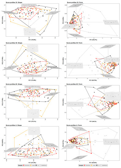
Figure 2.
PCA plots in shape and form space on the 7-landmark model at 35%, 50%, and 65% cross-sectional score length, and at the most conspicuous U-shaped score section. Extreme changes in shape and form along PC1 and PC2 are illustrated with the aid of transformation grids.
Table 2.
MANOVA p-values obtained on the 7-landmark models used to describe the score cross-sections at different lengths. Statistical significance (p < 0.003) is marked in bold.
Table 3.
Accuracy percentages >50% and kappa values (in parentheses) obtained for the different landmark (lm) and semilandmark (smlm) models generated for the present study, using gradient boosted machine (GBM), Support Vector Machine (SVM), Tree, and Neural Network (NN) algorithms.
PCA plots in shape space (Figure 2) suggest that leopards and lions are capable of generating a wider range of score morphologies in comparison to hyenas, considering the shape variability of the scores left by brown hyenas is the most limited one. On the contrary, when size is considered alongside shape, spotted hyenas present the largest form variance, probably directly associated with the large size range of the scores produced by this group (Figure S6). Spotted hyenas are capable of generating the most wide, superficial, and regular scores, among the studied carnivore species. Felid scores, on the other hand, tend to be deeper than hyaenid scores, although lions show a larger variance range depending on the score portion selected for the analysis.
Numerical results obtained for group mean comparison (Table 2) and classification purposes (Table 3) suggest that a sample including cross-sectional profiles at 35% of the total score length seems to be slightly more effective for carnivore group separation than score portions at 50% and 65% of the total score length, and significantly more efficient than morphological features captured in the most characteristic U-shaped score cross-section. However, even if distinguishing between group means based on morphological data obtained on the seven-landmark model seems plausible, only few ML algorithms are able to accurately classify more than 50% of the carnivore sample (Table 3), and only one of the tested GBM models on the seven-landmark models at 35% score length surpasses the 75% of accuracy.
3.2. The Semilandmark Models
3.2.1. Semilandmarks Models along One Curve
Results on the semilandmark models on a single curve, that is, without specifying the deepest point, are less conclusive than the results on the seven-landmark model, regardless of the number of points included in the model—10, 25, and 50—and the data processing approach—GM or EFA.
Although differences among carnivore groups are less marked, graphical results (Figure 3, Figure 4 and Figure 5) show similar trends as those observed in Figure 2, with lions and leopards displaying a wider shape variance in their tooth scores in opposition to hyenas, especially brown hyenas. Meanwhile, spotted hyenas and lions present the widest form variance, with the former group being characterized by its ability to generate quite shallow and homogeneous score cross-sectional profiles.
MANOVA results (Table 4 and Table 5) on the PC scores obtained after dimension reduction on GPA and EFA data highlight a significant decrease in group differentiation, especially when considering shape variables. Spotted hyenas usually present the greatest difficulties in being separated from the rest of the carnivore groups in shape space, while they are the only distinguishable group in form space.
Table 4.
MANOVA p-values obtained on the 10, 25, and 50 semilandmark (smlm) models used to describe the cross-sections at 50% of the score length. Statistical significance (p < 0.003) is marked in bold.
Table 5.
MANOVA p-values obtained on the 10, 25, and 50 semilandmark (smlm) models used to describe the cross-sections at 50% of the score length, using an EFA approach. Statistical significance (p < 0.003) is marked in bold.
ML and NN models used to analyze the performance of the semilandmark models for carnivore score characterization also decrease in accuracy when compared with the seven-landmark models. Table 2 presents mediocre results in carnivore group differentiation that only very rarely exceed 60% of accuracy.

Figure 3.
PCA plots in shape and form space on the single-curve semilandmark models at 50% cross-sectional score length, using 10 points; 25 points; and 50 points. Extreme changes in shape and form along PC1 and PC2 are illustrated with the aid of transformation grids.
Figure 3.
PCA plots in shape and form space on the single-curve semilandmark models at 50% cross-sectional score length, using 10 points; 25 points; and 50 points. Extreme changes in shape and form along PC1 and PC2 are illustrated with the aid of transformation grids.


Figure 4.
Shape PCA plots on Elliptic Fourier Analysis on the single-curve semilandmark models at 50% cross-sectional score length, using (a) 10 points; (b) 25 points; and (c) 50 points. Extreme changes in shape along PC1 and PC2 are illustrated with the aid of transformation grids. Optimal harmonics for each model are (a) 2; (b) 6; and (c) 6.


Figure 5.
Form PCA plots on Elliptic Fourier Analysis on the single-curve semilandmark models at 50% cross-sectional score length, using (a) 10 points; (b) 25 points; and (c) 50 points. Extreme changes in form along PC1 and PC2 are illustrated with the aid of transformation grids. Optimal harmonics for each model are (a) 2; (b) 6; and (c) 6.

3.2.2. Semilandmark Models along Two Curves
Semilandmark models along two curves, that is, considering the deepest point of the score cross-section, resemble the graphical results observed for the seven-landmark model more than when using a single curve (Figure 6 and Figure S7). Such results suggest that the incorporation of the deepest score point might be relevant for tooth score characterization. PCAs also highlight the existence of slight differences in the morphological definition of carnivore tooth scores with regard to the score portion selected for the study, either at score mid-length (50% of total mark length) or at the most conspicuous U-shaped score profile.
In comparison to the single curve semilandmark model, the inclusion of three fixed points, being one of them the deepest point on the score cross-section, helps to slightly improve group separation, particularly in form space (Table 6). Prediction models are, however, similarly ineffective to classify felids and hyenids based on the tooth scores they generate (Table 3).
Table 6.
MANOVA p-values obtained on the 13, 23, and 33 semilandmark (smlm) models on two curves used to describe the most conspicuous U cross-sections of the carnivore scores. Statistical significance (p < 0.003) is marked in bold.

Figure 6.
PCA plots in shape and form space on the 2-curves semilandmark models at the most conspicuous U score section, made by 13 points; 23 points; and 33 points. Extreme changes in shape and form along PC1 and PC2 are illustrated with the aid of transformation grids.
Figure 6.
PCA plots in shape and form space on the 2-curves semilandmark models at the most conspicuous U score section, made by 13 points; 23 points; and 33 points. Extreme changes in shape and form along PC1 and PC2 are illustrated with the aid of transformation grids.

Fourier Analyses do not present significant differences when compared to the single curve semilandmark models or with the analyses performed on the GM data. The characterization of the lion, leopard, and brown and spotted hyena tooth scores observed in Figure 7 and Figure 8 (also in Figures S8 and S9) follow the same trends of intraspecific variance observed in Figure 2, Figure 3, Figure 4, Figure 5 and Figure 6. Nevertheless, it is interesting to note certain differences in group differentiation depending on the score portion included in the study and the data processing, since the EFA approach on the most conspicuous U-shaped portion of the score profile (Table 7) generates the best and most consistent results for the separation of brown hyenas based on shape data from the remaining carnivores included in the present study. In form space, apart from the constant clear separation of spotted hyenas, brown hyenas appear to be more easily distinguishable than felids. These differences are, however, not reflected in the classification models conducted on ML and NN algorithms (Table 3).
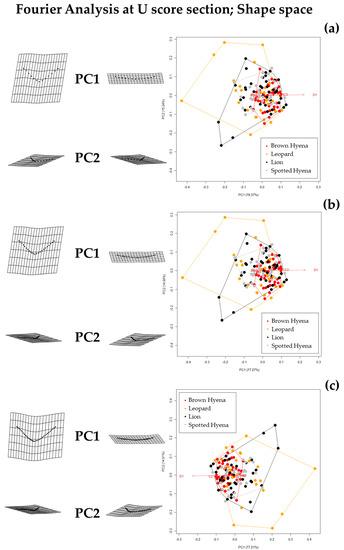
Figure 7.
Shape PCA plots on Elliptic Fourier Analysis on the 2-curves semilandmark models at the most conspicuous U score section, using (a) 13 points; (b) 23 points; and (c) 33 points. Extreme changes in shape along PC1 and PC2 are illustrated with the aid of transformation grids. Optimal harmonics for each model are (a) 4; (b) 6; and (c) 6.
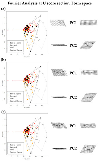
Figure 8.
Form PCA plots on Elliptic Fourier Analysis on the 2-curves semilandmark models at the most conspicuous U score section, using (a) 13 points; (b) 23 points; and (c) 33 points. Extreme changes in form along PC1 and PC2 are illustrated with the aid of transformation grids. Optimal harmonics for each model are (a) 4; (b) 6; and (c) 6.
Table 7.
MANOVA p-values obtained on the 13, 23, and 33 semilandmark (smlm) models on two curves used to describe the most conspicuous U cross-sections of the carnivore scores, using an EFA approach. Statistical significance (p < 0.003) is marked in bold.
4. Discussion
Tooth scores are elongated U-shaped marks that are commonly found on the cortical surfaces of skeletons modified by carnivores [1,17]. The first attempt to analyse score morphology using GM techniques was based on a seven-landmark model that provided promising results in the differentiation of carnivore groups [19]. However, methodological laxity regarding the selection of the score profile and the subsequent potential lack of representativeness of such cross-sections required a more detailed study, including the morphological comparison of score profiles at different score lengths. The conduction of thorough methodological research, like the one presented here, has not only allowed the evaluation of intra-specific score morphological variation and cross-sectional representativeness, but also demonstrated the effectiveness of landmark and semilandmark models for the differentiation of carnivore families and taxa based on specific cases.
Results show that the selection of the cross-sectional portion does not greatly affect the morphological characterization of the tooth scores produced by lions, leopards, and spotted and brown hyenas, as intra-specific variation does not seem to vary significantly (Figure S5). However, according to the tests performed here, the discrimination between carnivore groups improves when the sections selected for the present study (e.g., 35/50/65%) are used, instead of the most conspicuous U-shape section [19] (Table 2). This is particularly striking in the case of different carnivore families (e.g., hyenids and felids). Thus, a standardization of the model considering specific profiles along the score length might not only help replicate the method, but might also improve discrimination among carnivore groups.
However, when comparing the effect of the selection of different standardized cross-sections, it appears that not all cross-sections are equally valid for carnivore characterization and group separation. For instance, species discrimination slightly improves when the 35% profile is selected (Table 2). Since 35% and 65% profiles are the result of score orientation and are, thus, randomly grouped as such, it can only be hypothesized that the score ends (e.g., 35% and 65%) may be more suitable for morphological characterization than profiles at half score length (50%). However, analyses considering 65% profiles highlight that lions and leopards cannot be statistically differentiated, neither in shape nor in form space, while brown and spotted hyenas can only be distinguished in form space. These results suggest that score size is important in order to characterize hyenid species. In fact, spotted hyenas present the largest form variance, probably directly associated with the large size range of the scores they produce (Figure S6). In sum, the seven-landmark model first published by [19] is able to differentiate between hyenid species in form space, but cannot distinguish between felid species neither in shape nor in form space. Nevertheless, if carnivore species are grouped by family (e.g., Felidae and Hyenidae), groups can be statistically differentiated both in shape and form space.
These results are important for taphonomic studies, since different carnivores may modify and accumulate bones in archaeopaleontological contexts. Additionally, distinguishing the action of felids and hyenids in archaeological sites is also particularly relevant in order to clarify the anthropogenic access order to animal carcasses in those sites where both human and carnivore action has been recognized. It has been hypothesized that felid species may provide ungulate carcasses for human scavenging [8,17]. In contrast, hyenid species usually consume their prey entirely [67,68]. Thus, if the main carnivore activity at a specific site can be classified as felid-made, there is a possibility that humans may have secondarily intervened, scavenging the skeletal parts previously consumed by felids. On the contrary, if carnivore tooth marks are mainly classified as hyenid-made, this means that the bone assemblage may have been first modified by humans and subsequently scavenged by hyenas.
Furthermore, the methodology tested here is able to differentiate between brown and spotted hyenas based on the form of the scores they generate. This is particularly important because both hyenid species are able to produce bone accumulations. It has been proposed that numerous paleontological sites worked as hyena dens both in Africa and Europe during the Pleistocene. Previous research has explored several taphonomic variables in order to distinguish bone assemblages accumulated by different hyenid species, although not without problems, since hyenids may produce similar taphonomic modifications that impede the discrimination among taxa [69,70]. The application of the seven-landmark method can shed light on these equifinality problems and help discern the action of specific hyenid species at paleontological sites. The generalization of this hypothesis, however, requires additional analyses. Striped hyenas, which were not included in the present study, can also produce bone accumulations. Thus, in order to prove useful to the discrimination among all living and skilled bone-accumulator hyenid taxa, the seven-landmark model needs to be tested on spotted, brown, and stripped hyenas.
In addition to the fine-tuning of the already published seven-landmark method [19], in the present study, we have assessed novel models based on semilandmarks for the characterization and analysis of tooth scores. First, we have explored if the inclusion of a higher number of points provides a better registration of score morphology and, thus, an improvement in carnivore differentiation.
Models including 10, 25, and 50 semilandmarks on a single curve, that is, without specifying the deepest point of the score profile, were evaluated showing similar general morphological trends to the seven-landmark method, but a lower differentiation power between groups (Table 2, Table 4 and Table 5). Conversely to the seven-landmark method, these novel models are not able to distinguish between felids and hyenids, regardless of the methodological approach, namely using GM and EFA approaches. In fact, only hyenid species can be statistically differentiated when shape and size features are considered together, confirming that brown and spotted hyenas are morphologically easier to discriminate than lions and leopards, probably due to the differences in size observed between the former species (Figure S6).
The second group of models based on semilandmarks (13, 23, and 33) was molded using two curves that end at the score profile lateral ends and the deepest point of the score cross-section. Results show that the differentiation power improves when using the two-curve models in comparison to the one-curve models, which suggests that the deepest point may be morphologically relevant to describe score morphology. Nevertheless, carnivore distinction is still less clear than using the original seven-landmark model, since the two-curve models are not able to consistently separate felids from hyenids based on the tooth scores they generate, and can only statistically distinguish between brown and spotted hyenas in form space, like the rest of the models tested in the present study (Table 6). Additionally, the EFA approach is also capable of separating the brown hyena sample from the rest of the carnivore groups included in the study when considering only shape variables (Table 7). However, this is likely due to the number of variables used in the analysis, which would result in an increase of the effects of the curse of dimensionality.
In general, the results obtained here highlight that the use of high numbers of landmarks to describe tooth score cross-sections does not necessarily improve morphological characterization and carnivore differentiation. Thus, the use of semilandmark models is not recommended for the study of archaeopaleontological sites where both felid and hyenid may have acted as taphonomic agents. Anyway, in case of using 2D semilandmark curves to avoid landmarking biases, researchers might want to make sure that the deepest point of the score cross-section is included in the analysis, as its location seems to be relevant for morphological characterization.
Among the carnivores included in the study, hyenids seem to be easier to differentiate based on the tooth score morphology they generate, probably with reference to the effect that size has on the spotted hyena score morphology. Spotted hyenas form, indeed, the most differentiated group (see balanced accuracy in Table S2), whereas leopards usually present the lowest accuracy rates among the four groups. Thus, while the 3D GMM analysis of carnivore pits has provided useful tools for the separation of carnivores, including the distinction of leopards and lions [26], as well as wider range of carnivore taxa [20,21,22,23], the GMM analysis of score morphology might be relevant for the distinction of not only hyenid species, but also different carnivore families in those scenarios, where the tooth pit sample is not large enough to perform statistical analyses due to preservation problems.
Despite the positive results obtained regarding the separation among hyenid species, further analyses are required to prove the validity of the method in a more generalized context that includes a wider range of carnivore taxa. Therefore, works in this line including 2D and 3D landmark data will be conducted in the following years.
5. Conclusions
Different landmark-based models have been tested to explore the discrimination power of tooth score morphology inflicted by felid and hyenid species, while considering the effect that the score portion might have on group characterization. Although some differences have been observed depending on where cross-sectional profiles are taken, no significant intra-specific differences have been observed, which allows the replication of the methodology. Among the landmark models assessed in the present study, the seven-landmark method achieved the most consistent results, since it is capable of differentiating between hyenids and felids when the profile cross-sections are standardized, both in shape and form space. In contrast, scores produced by hyenids and felids are not consistently distinguished through any semilandmark method, either when they are slid on one or two curves, and regardless of the number of semilandmarks used. Only hyenid species can be consistently discriminated in form space when models include low number of points and consider the deepest point of the score cross-section. That is why, out of the semilandmark models tested here, the use of the 13-semilandmark model that includes two curves is the most recommended one. Further research is needed to assess the methodology using a wider range of carnivore families (e.g., canids), as well as to explore the possibilities that 3D methods might provide regarding the registration and analysis of tooth scores.
Supplementary Materials
The following supporting information can be downloaded at: https://www.mdpi.com/article/10.3390/app13063864/s1, Supplementary File S1: Results; containing additional figures (Figures S1–S9) and tables (Tables S1 and S2).
Author Contributions
Conceptualization, M.C.A. and J.A.; Methodology, J.A. and L.A.C.; Software, L.A.C.; Validation, M.C.A. and J.A.; Formal analysis, M.C.A. and J.A.; Investigation, M.C.A. and J.A.; Resources, M.C.A. and J.Y.; Data curation, M.C.A., M.Á.M.-G. and D.H.-R.; Writing—original draft, M.C.A. and J.A.; Writing—review and editing, M.C.A., J.A. and L.A.C.; Visualization, M.C.A. and J.A.; Supervision, M.C.A. and J.A.; Project administration, M.C.A., D.G.-A. and J.Y.; Funding acquisition, M.C.A., D.G.-A. and J.Y. All authors have read and agreed to the published version of the manuscript.
Funding
The grant IJC2020-043576-I funded by MCIN/AEI/10.13039/501100011033 and the “European Union NextGenerationEU/PRTR” has been awarded to M.C.A. The grant RYC2021-034813-I funded by MCIN/AEI/10.13039/501100011033 and the European Union “NextGenerationEU”/PRTR has been awarded to M.Á.M.-G. During the development of the present work, J.A. was funded by the Euskal Herriko Unibertsitatea [ESPDOC21/05]. L.A.C. is funded by the Spanish Ministry of Science, Innovation and Universities by an FPI Predoctoral grant PRE2019-089411 associated with project RTI2018-099850-B-I0.
Institutional Review Board Statement
No animals were sacrificed specifically for the purpose of these experiments. Carnivores were not manipulated or handled at any point throughout the collection of samples. No licenses or permits were required to perform these experiments.
Informed Consent Statement
Not applicable.
Data Availability Statement
All relevant data are within the paper and its Supporting Information file. The R code used for the present study is freely available on L.A.C. GitHub page (https://github.com/LACourtenay/tooth_score_digitisation accessed on 13 March 2023). The landmark data are available upon request.
Acknowledgments
We would like to thank the Ditsong Museum (Pretoria) and especially Heidi Fourie for providing access to Bob Brain’s neotaphonomic collections. We are also grateful for the support provided by the TIDOP Group in the Department of Cartographic and Land Engineering of the Higher Polytechnics School of Avila, University of Salamanca, and would like to thank them for using their tools and facilities.
Conflicts of Interest
The authors declare no conflict of interest. The funders had no role in the design of the study; in the collection, analyses, or interpretation of data; in the writing of the manuscript; or in the decision to publish the results.
References
- Binford, L.R. Bones Ancient Men and Modern Myths; New York Academic Press: New York, NY, USA, 1981. [Google Scholar]
- Brain, C.K. The Hunters or the Hunted? An Introduction to African Cave Taphonomy; Chicago University Press: Chicago, IL, USA, 1981. [Google Scholar]
- Bunn, H.T. Meat-Eating and Human Evolution: Studies on the Diet and Subsistence Patterns of Plio-Pleistocene Hominids in East Africa. Ph.D. Thesis, University of California, Berkeley, CA, USA, 1982. [Google Scholar]
- Klein, R.G. Age (mortality) profiles as a means of distinguishing hunted species from scavenged ones in Stone Age archaeological sites. Paleobiology 1982, 8, 151–158. [Google Scholar] [CrossRef]
- Shipman, P.; Rose, J.J. Early hominid hunting, butchering and carcass-processing behaviors: Approaches to the fossil record. J. Anthropol. Archaeol. 1983, 2, 57–98. [Google Scholar] [CrossRef]
- Blumenschine, R.J. Early Hominid Scavenging Opportunities. Implications of Carcass Availability in the Serengeti and Ngorongoro Ecosystems; British Archaeological Reports. International Series, 283; BAR Publishing: Oxford, UK, 1986. [Google Scholar]
- Domínguez-Rodrigo, M. Meat eating by early homids at FLK Zinj 22 Site, Olduvai Gorge Tanzania: An experimental a roach using cutmark data. J. Hum. Evol. 1997, 33, 669–690. [Google Scholar] [CrossRef] [PubMed]
- Blumenschine, R.J. An experimental model of the timing of hominid and carnivore influence on archaeological bone assemblages. J. Archaeol. Sci. 1988, 15, 483–502. [Google Scholar] [CrossRef]
- Bartram, L.E.; Marean, C.W. Explaining the “Klasies Pattern”: Kua ethnoarchaeology, the Die Kelders Middle Stone Age archaeofauna, long bone fragmentation and carnivore ravaging. J. Archaeol. Sci. 1999, 26, 9–29. [Google Scholar] [CrossRef]
- Pickering, T.R. Reconsideration of criteria for differentiating faunal assemblages accumulated by hyenas and hominids. Int. J. Osteoarchaeol. 2002, 12, 127–141. [Google Scholar] [CrossRef]
- Parkinson, J.; Plummer, T.; Hartstone-Rose, A. Characterizing felid tooth marking and gross bone damage patterns using GIS image analysis: An experimental feeding study with large felids. J. Hum. Evol. 2015, 80, 114–134. [Google Scholar] [CrossRef]
- Selvaggio, M.M. Identifying the Timing and Sequence of Hominid and Carnivore Involvement with Plio-Pleistocene Bone Assemblages from Carnivore Tooth Marks and Stone-Tool Butchery Marks on Bone Surfaces. Ph.D. Thesis, Rutgers University, New Brunswick, NJ, USA, 1994. [Google Scholar]
- Andrews, P.; Fernández-Jalvo, Y. Surface modifications of the Sima de los Huesos fossil humans. J. Hum. Evol. 1997, 33, 191–217. [Google Scholar] [CrossRef]
- Domínguez-Rodrigo, M.; Piqueras, A. The use of tooth pits to identify carnivore taxa in tooth-marked archaeofaunas and their relevance to reconstruct hominid carcass processing behaviours. J. Archaeol. Sci. 2003, 30, 1385–1391. [Google Scholar] [CrossRef]
- Delaney-Rivera, C.; Plummer, T.W.; Hodgson, J.A.; Forrest, F.; Hertel, F.; Oliver, J.S. Pits and pitfalls: Taxonomic variability and patterning in tooth mark dimensions. J. Archaeol. Sci. 2009, 36, 2597–2608. [Google Scholar] [CrossRef]
- Andrés, M.; Gidna, A.; Yravedra, J.; Domínguez-Rodrigo, M. A study of dimensional differences of tooth marks (pits and scores) on bones modified by small and large carnivores. Archaeol. Anthropol. Sci. 2012, 4, 209–219. [Google Scholar] [CrossRef]
- Blumenschine, R.J. Percussion marks, tooth marks and the experimental determinations of the timing of hominid and carnivore access to long bones at FLK Zinjanthropus, Olduvai Gorge, Tanzania. J. Hum. Evol. 1995, 29, 21–51. [Google Scholar] [CrossRef]
- Domínguez-Rodrigo, M.; Egeland, C.P.; Pickering, T.R. Equifinality in carnivore tooth marks and the extended concept of archaeological palimpsests: Implications for models of passive scavenging by hominids. In Breathing Life into Fossils: Taphonomic Studies in Honor of C.K. (Bob) Brain; Pickering, T.R., Schick, K., Toth, N., Eds.; Stone Age Institute Press: Bloomington, IN, USA, 2007; pp. 255–267. [Google Scholar]
- Yravedra, J.; García-Vargas, E.; Maté-González, M.A.; Aramendi, J.; Palomeque-González, J.F.; Vallés-Iriso, J.; Matesanz-Vicente, J.; González-Aguilera, D.; Domínguez-Rodrigo, M. The use of micro-photogrammetic and geometric-morphometry for identifying carnivore activity in the bone assemblages. J. Archaeol. Sci. Rep. 2017, 14, 106–115. [Google Scholar]
- Aramendi, J.; Maté-González, M.Á.; Yravedra, J.; Ortega, M.C.; Arriaza, M.C.; González-Aguilera, D.; Baquedano, E.; Domínguez-Rodrigo, M. Discerning carnivore agency through the three-dimensional study of tooth pits: Revisiting crocodile feeding behaviour at FLK- Zinj and FLK NN3 (Olduvai Gorge, Tanzania). Palaeogeogr. Palaeoclimatol. Palaeoecol. 2017, 488, 93–102. [Google Scholar] [CrossRef]
- Courtenay, L.A.; Yravedra, Y.; Huguet, R.; Aramendi, J.; Maté-González, M.Á.; González-Aguilera, D.; Arriaza, M.C. Combining machine learning algorithms and geometric morphometrics: A study of carnivore tooth marks. Palaeogeogr. Palaeoclimatol. Palaeoecol. 2019, 522, 28–39. [Google Scholar] [CrossRef]
- Courtenay, L.A.; Herranz-Rodrigo, D.; Huguet, R.; Maté-González, M.Á.; González-Aguilera, D.; Yravedra, J. Obtaining new resolutions in carnivore tooth pit morphological analyses: A methodological update for digital taphonomy. PLoS ONE 2020, 15, e0240328. [Google Scholar] [CrossRef]
- Courtenay, L.A.; Herranz-Rodrigo, D.; González-Aguilera, D.; Yravedra, J. Developments in data science solutions for carnivore tooth pit classification. Sci. Rep. 2021, 11, 10209. [Google Scholar] [CrossRef] [PubMed]
- Domínguez-Rodrigo, M.; Yravedra, J.; Organista, E.; Gidna, A.; Fourvel, J.B.; Baquedano, E. A new methodological approach to the taphonomic study of paleontological and archaeological faunal assemblages: A preliminary case study from Olduvai Gorge (Tanzania). J. Archaeol. Sci. 2015, 59, 35–53. [Google Scholar] [CrossRef]
- Gidna, A.; Yravedra, J.; Domínguez-Rodrigo, M. A cautionary note on the use of captive carnivores to model wild predator behavior: A comparison of bone modification patterns on long bones by captive and wild lions. J. Archaeol. Sci. 2013, 40, 1903–1910. [Google Scholar] [CrossRef]
- Arriaza, M.C.; Aramendi, J.; Maté-González, M.Á.; Yravedra, J.; Stratford, D. Characterising leopard as taphonomic agent through the use of micro-photogrammetric reconstruction of tooth marks and pit to score ratio. Hist. Biol. 2021, 33, 176–185. [Google Scholar] [CrossRef]
- Arriaza, M.C.; Aramendi, J.; Maté-González, M.Á.; Yravedra, J.; Stratford, D. The hunted or the scavenged? Australopith accumulation by brown hyenas at Sterkfontein (South Africa). Quat. Sci. Rev. 2021, 273, 107252. [Google Scholar] [CrossRef]
- González-Aguilera, D.; López-Fernández, J.; Rodríguez-González, P.; Hernández-López, D.; Guerrero-Sevilla, D.; Remondino, F.; Menna, F.; Nocerino, E.; Toschi, I.; Ballabeni, A.; et al. GRAPHOS—Open-source software for photogrammetric applications. Photogramm. Rec. 2019, 33, 11–29. [Google Scholar] [CrossRef]
- Fraser, C.S. Multiple focal setting self-calibration of close-range metric cameras. Photogramm. Eng. Remote Sens. 1980, 46, 1161–1171. [Google Scholar]
- Maté-González, M.Á.; Yravedra, J.; González-Aguilera, D.; Palomeque-González, J.F.; Domínguez-Rodrigo, M. Micro-photogrammetric characterization of cut marks on bones. J. Archaeol. Sci. 2015, 62, 128–142. [Google Scholar] [CrossRef]
- O’Higgins, P.; Johnson, D.R. The quantitative description and comparison of biological forms. Crit. Rev. Anat. Sci. 1988, 1, 149–170. [Google Scholar]
- Bookstein, F.L. Morphometric Tools for Landmark Data: Geometry and Biology; Cambridge University Press: New York, NY, USA, 1991. [Google Scholar]
- Hall, B.K. Descent with modification: The unity underlying homology and homoplasy as seen through an analysis of development and evolution. Biol. Rev. 2003, 78, 409–433. [Google Scholar] [CrossRef] [PubMed]
- Klingenber, C.P. Novelty and “homology-free” morphometrics: What’s in a name? Evol. Biol. 2008, 35, 186–190. [Google Scholar] [CrossRef]
- Rohlf, F.J. Shape statistics: Procrustes superimpositions and tangent spaces. J. Classif. 1999, 16, 197–223. [Google Scholar] [CrossRef]
- Slice, D.E. Landmark coordinates aligned by procrustes analysis do not lie in Kendall’s shape space. Syst. Biol. 2001, 50, 141–149. [Google Scholar] [CrossRef]
- Richtsmeier, J.T.; Deleon, V.B.; Lele, S.R. The promise of geometric morphometrics. Am. J. Phys. Anthropol. 2002, 119, 63–91. [Google Scholar] [CrossRef]
- Bookstein, F.L. Landmark methods for forms without landmarks: Morphometrics of group differences in outline shape. Med. Image Anal. 1997, 1, 225–243. [Google Scholar] [CrossRef] [PubMed]
- Gunz, P.; Mitteroecker, P. Semilandmarks: A method for quantifying curves and surfaces. Hystrix Ital. J. Mammal. 2013, 24, 103–109. [Google Scholar]
- R Core Team. A Language and Environment for Statistical Computing; R Foundation for Statistical Computing: Vienna, Austria, 2015; Available online: https://www.Rproject.org/ (accessed on 1 December 2022).
- Courtenay, L.A. Tooth Score Digitisation Tools; Github: San Francisco, CA, USA, 2022; Available online: https://github.com/LACourtenay/tooth_score_digitisation (accessed on 2 February 2023).
- Adams, D.; Collyer, M.; Kaliontzopoulou, A.; Baken, E. Geomorph: Geometric Morphometric Analyses of 2D/3D Landmark Data, R Package, Version 4.0.5; R Foundation for Statistical Computing: Vienna, Austria, 2020; Available online: https://cran.r-project.org/web/packages/geomorph/index.html (accessed on 1 December 2022).
- Bookstein, F.L. Principal warps: Thin-plate spline and the decomposition of deformations. IEEE Trans. Pattern Anal. Mach. Intell. 1989, 11, 567–585. [Google Scholar] [CrossRef]
- Courtenay, L.A. GraphGMM, v.1.0.0; Github: San Francisco, CA, USA, 2022; Available online: https://github.com/LACourtenay/GraphGMM (accessed on 2 February 2023).
- Murrell, P. R Graphics; Chapman & Hall/CRC Press: Boca Raton, FL, USA, 2005. [Google Scholar]
- Wickham, H. ggplot2: Elegant Graphics for Data Analysis; Springer: New York, NY, USA, 2016. [Google Scholar]
- Courtenay, L.A.; Barbero-García, I.; Aramendi, J.; González-Aguilera, D.; Rodríguez-Martín, M.; Rodríguez-Gonzalvez, P.; Cañueto, J.; Román-Curto, C. A Novel Approach for the Shape Characterisation of Non-Melanoma Skin Lesions Using Elliptic Fourier Analyses and Clinical Images. J. Clin. Med. 2022, 11, 4392. [Google Scholar] [CrossRef]
- Engda Redae, B.; Courtenay, L.A.; Souron, A.; Costamagno, S.; Rozada, L.; Parkinson, J.; Drumheller, S.; Delagnes, A.; Boisserie, J.R.; Lesur, J. Identifying taphonomic agents from the Plio-Pleistocene record of the Shungura Formation (lower Omo River Valley, Ethiopia) using confocal microscopy and Elliptic Fourier Analyses. In Proceedings of the TAPHOS-ICAZ 9th International Meeting on Taphonomy and Fossilization, Madrid, Spain, 5–11 June 2022. [Google Scholar]
- Giardina, C.R.; Kuhl, F.P. Accuracy of curve approximation by harmonically related vectors with elliptical loci. Comput. Graph. Image Process. 1977, 6, 277–285. [Google Scholar] [CrossRef]
- Kuhl, F.P.; Giardina, C.R. Elliptic Fourier features of a closed contour. Comput. Graph. Image Process. 1982, 18, 236–258. [Google Scholar] [CrossRef]
- Rohlf, F.J. Fitting curves to outlines. In the Michigan Morphometrics Workshop; Rohlf, F.J., Bookstein, F.L., Eds.; The University of Michigan Museum of Zoology: Arbor, MI, USA, 1990; pp. 167–177. [Google Scholar]
- Ferson, S.; Rohlf, F.J.; Koehn, R.K. Measuring Shape Variation of Two-dimensional Outlines. Syst. Biol. 1985, 34, 59–68. [Google Scholar] [CrossRef]
- Mohd Razali, N.; Bee Wah, Y. Power comparisons of Shapiro-Wilk, Kolmogorov-Smirnov, Lilliefors and Anderson-Darling tests. J. Stat. Model. Anal. 2011, 2, 21–33. [Google Scholar]
- Courtenay, L.; Gonzalez-Aguilera, D.; Lagüela, S.; del Pozo, S.; Ruiz Méndez, C.; Barbero-García, I.; Román-Curto, C.; Cañueto, J.; Santos-Durán, C.; Cardeñoso-Álvarez, M.E.; et al. Hyperspectral Imaging and Robust Statistics in Non-Melanoma Skin Cancer Analysis. Biomed. Opt. Express 2021, 12, 5107–5127. [Google Scholar] [CrossRef]
- Höhle, J.; Höhle, M. Accuracy assessment of digital elevation models by means of robust statistical methods. ISPRS J. Photogramm. Remote Sens. 2009, 64, 398–406. [Google Scholar] [CrossRef]
- Rao, C.R. An asymptotic expansion of the distribution of Wilk’s criterion. Bull. Int. Stat. Inst. 1951, 33, 177–180. [Google Scholar]
- Hervé, M. “RVAideMemoire” Package: Testing and Plotting Procedures for Biostatistics. Version 0.9-81-2. 2022. Available online: https://cran.r-project.org/web/packages/RVAideMemoire/RVAideMemoire.pdf (accessed on 1 December 2022).
- Hothorn, T.; Hornik, K.; Strobl, C.; Zeileis, A. “Party” Package: A Laboratory for Recursive Partytioning. Version 1.3.-11. 2022. Available online: https://cran.r-project.org/web/packages/party/party.pdf (accessed on 1 December 2022).
- Kuhn, M. “Caret” Package: Classification and Regression Training. R Package. Version 6.0-93. 2022. Available online: https://cran.r-project.org/web/packages/caret/caret.pdf (accessed on 1 December 2022).
- Cortes, C.; Vapnik, V. Support-vector networks. Mach. Learn. 1995, 20, 273–297. [Google Scholar] [CrossRef]
- Snoek, J.; Larochelle, H.; Adams, R.P. Practical Bayesian Optimization of Machine Learning Algorithms. arXiv 2012, arXiv:1203.2944. [Google Scholar]
- Shahriari, B.; Swersky, K.; Wang, Z.; Adams, R.P.; De Freitas, N. Taking the human out of the loop: A review of Bayesian optimization. Proc. IEEE 2016, 104, 148–175. [Google Scholar] [CrossRef]
- Bergstra, J.; Bengio, Y. Random Search for Hyper-Parameter Optimization Yoshua Bengio. J. Mach. Learn. Res. 2012, 13, 281–305. [Google Scholar]
- Bergstra, J.; Bardenet, R.; Bengio, Y.; Kégl, B. Algorithms for Hyper-Parameter Optimization. Int. Conf. Neural Inf. Process. Syst. 2011, 24, 2546–2554. [Google Scholar]
- Lantz, B. Machine Learning with R; Packt Publishing Ltd.: Birmingham, UK, 2013. [Google Scholar]
- Venables, W.N.; Ripley, B.D. Modern Applied Statistics with S; Springer: New York, NY, USA, 2002. [Google Scholar]
- Kruuk, H. The Spotted Hyena: A Study of Predation and Social Behavior; Chicago University Press: Chicago, IL, USA, 1972. [Google Scholar]
- Sutcliffe, A.J. Spotted hyaena: Crusher, gnawer, digester and collector of bones. Nature 1970, 227, 1110–1113. [Google Scholar] [CrossRef]
- Fosse, P.; Avery, G.; Fourvel, J.B.; Lesur-Gebremariam, J.; Monchot, H.; Brugal, J.P.; Kolska Horwitz, L.; Tournepiche, J.F. Los cubiles actuales de hiena: Sintesis criteria de sus caracteristicas tafonómicas a partir de la excavacion de nuevos yacimientos (Republica de Djibuti, Africa del Sur) y la informacion publicada. In Actas de la Primera Reunion de Cientificos Sobre Cubiles de Hiena (y Otros Grandes Carnivoros) en los Yacimientos Arqueológico de la Peninsula Iberica; Rosell, J., Baquedano, E., Eds.; Museo Arqueologico Regional de la Comunidad de Madrid, Alcala de Henares: Madrid, Spain, 2010; pp. 108–117. [Google Scholar]
- Fourvel, J.P.; Fosse, P.; Avery, G. Spotted, striped or brown? Taphonomic studies at dens of extant hyaenas in eastern and southern Africa. Quat. Int. 2015, 369, 38–50. [Google Scholar] [CrossRef]


Disclaimer/Publisher’s Note: The statements, opinions and data contained in all publications are solely those of the individual author(s) and contributor(s) and not of MDPI and/or the editor(s). MDPI and/or the editor(s) disclaim responsibility for any injury to people or property resulting from any ideas, methods, instructions or products referred to in the content. |
© 2023 by the authors. Licensee MDPI, Basel, Switzerland. This article is an open access article distributed under the terms and conditions of the Creative Commons Attribution (CC BY) license (https://creativecommons.org/licenses/by/4.0/).