Analysis of the Failure Area of the Slope Using the Slip Line Method

Abstract

Most geotechnical engineers focus on ground strength and stability. However, when determining stability by analyzing the exact strength of the ground, the failure surface is essential. Nevertheless, limited studies have been conducted on the methods to determine the exact failure surface of the ground. This study shows that the failure surface and plastic area can be analyzed using the slip line method based on the slip line and lower bound analysis. To improve existing studies limited to single ground, we analyzed the failure area of heterogeneous ground conditions. The results of the slip line method were compared and verified through FELM, a finite element analysis method to which a lower limit analysis was applied. As a result, the failure area and maximum internal stress according to the ground properties and the slope angle are presented. In addition, the points of the slip line method and the finite element limit analysis are summarized. Finally, we propose limitations and solutions when applying the slip line method to the slope.

1. Introduction

Various theories and methods for determining the strength of the ground have been proposed in the field of geotechnical engineering. Based on these theories, various design and construction methods are applied to structures. While various studies have been conducted to determine the strength of the ground, limited studies have been conducted on the methods to determine the exact failure surface of the ground. For slope stability analysis, it is necessary to determine the failure surface. However, it is difficult to determine the failure surface by considering various factors, and most failure surfaces are estimated via the empirical judgment of engineers. Therefore, estimations of failure surfaces are unreliable. Based on these reasons, research on failure surface analysis is necessary.

Research to determine the failure surface has been mainly conducted using algorithms. In the 2000s, global optimization methods were studied in research on critical failure surfaces. Bolton et al. conducted a study to determine the critical failure surface using a global optimization algorithm [1]. Cheng carried out a study using simulated annealing, a probabilistic heuristic method, to identify the critical failure surface [2]. Cheng et al. conducted a study to determine the critical non-circular failure surface through the particle cluster optimization algorithm [3]. Kahatadeniya et al. conducted a study to determine the critical failure surface using ant colony optimization, a method of artificial neural networks [4]. Himanshu et al. conducted a study to determine the critical failure surface through the gray wolf optimization approach, which is a type of global optimization method [5]. Khajehazadeh et al. conducted a seismic analysis of an earth slope using a novel sequential hybrid optimization algorithm [6].

Equally, researchers studied finding the critical failure surface through genetic algorithms. Zolfaghari et al. conducted a study to determine the critical non-circular failure surface through a simple genetic algorithm [7]. Li et al. conducted a study to determine the critical failure surface using a hybrid genetic algorithm [8]. Sengupta and Upadhyay conducted a study to determine the critical failure surface through a search method based on a genetic algorithm under general conditions with constraints [9].

In addition, Zhang and Zhang recently conducted a study to determine the critical failure surface of a slope by combining a two-dimensional ordinary-state-based peridynamic (OSB-PD) plastic model with the Drucker–Prager criterion [10].

These studies can reflect various conditions as a mechanism for presenting a failure surface by learning failure conditions, but many conditions are required to analyze the failure.

Meanwhile, other researchers studied the failure area mechanism through upper and lower limit analysis among limit analysis methods.

Zhang et al. studied the failure area mechanism using limit analysis and presented the tunnel’s failure area and limit support pressure [11]. Li et al. conducted a study on the failure mechanism considering the kinematically acceptable soil arcuate velocity field [12]. Tu et al. proposed a new failure mechanism that improved the spatial discretization technique to evaluate the stability of tunnel surfaces in inclined strata based on the upper limit analysis method [13].

Shiau et al. conducted a study on the three-dimensional (3D) undrained slopes in anisotropic and heterogeneous clay using advanced upper- and lower-bound finite element limit analysis (FELA). Using the multivariate adaptive regression splines (MARS) analysis, the respective influence and sensitivity of each design parameter on the stability number and the failure mechanism were investigated [14]. Yodsomjai et al. presented new plasticity solutions for undrained stability of unsupported conical slopes in two-layered clays by using axisymmetric finite element limit analysis [15]. Yodsomjai et al. presented new plasticity stability solutions for an unsupported conical rock slope through a finite element limit analysis framework [16]. Lai et al. studied the seismic bearing capacity of the strip foundation on a cohesive soil slope, and various landfill depths were investigated through finite element limit analysis [17].

In contrast, studies using slip line focused on estimating ground-bearing capacity rather than searching for failure surfaces. Martin developed a program to determine the ground-bearing capacity of foundations using the slip line method [18]. Gao et al. (2015) studied slip line field solutions for the extreme bearing capacity of pipelines in drained soils [19]. Liu and Chen studied the shearing characteristics of slip zone soils and strain localization analysis of a landslide [20]. Keshavarz studied the seismic bearing capacity of strip foundations on rock formations using the Hoek–Brown failure criterion [21]. Zhou et al. conducted a slip-line-theory-based stability analysis on the effect of deep excavation on adjacent slopes [22]. Tesgaya studied the bearing capacity of shallow foundations located at various distances from a slope [23]. Park and Han studied the acupressure analysis of the tunnel ceiling according to the tunnel plastic zone [24] and Lee studied the failure load calculation of the V-shaped rock notch using the slip line method [25].

In terms of solid mechanics, Hill (1950) studied plasticity by numerical analysis using the slip line method [26]. In terms of soil mechanics, the study of failure surfaces using the slip line method was initiated by Sokolovski [27]. Sokolovski analyzed the cases where there is unit weight and internal friction angle (γ ≠ 0 and Φ ≠ 0), which are general geometric conditions in the slip line method, in a study to find the failure surface using the slip line [27]. However, they could not solve the equation; therefore, they analyzed it through a numerical method (finite difference method).

Based on the studies of Sokolovski, Wang et al. applied the slip line method to single ground using Excel spreads to analyze the plasticity area [28].

In this study, to improve existing studies limited to single ground and methodological errors of the slip line method, we applied failure surface analysis using the slip line method to heterogeneous ground with reference to the research of Wang et al. and Sokolovski. In addition, we conducted a finite element limit analysis (strength reduction method), similar to the slip line method, and a comparative analysis to emphasize the features of the slip line method. Based on these results, this paper presents a failure surface determination method using the slip line method.

2. Slip Line Method

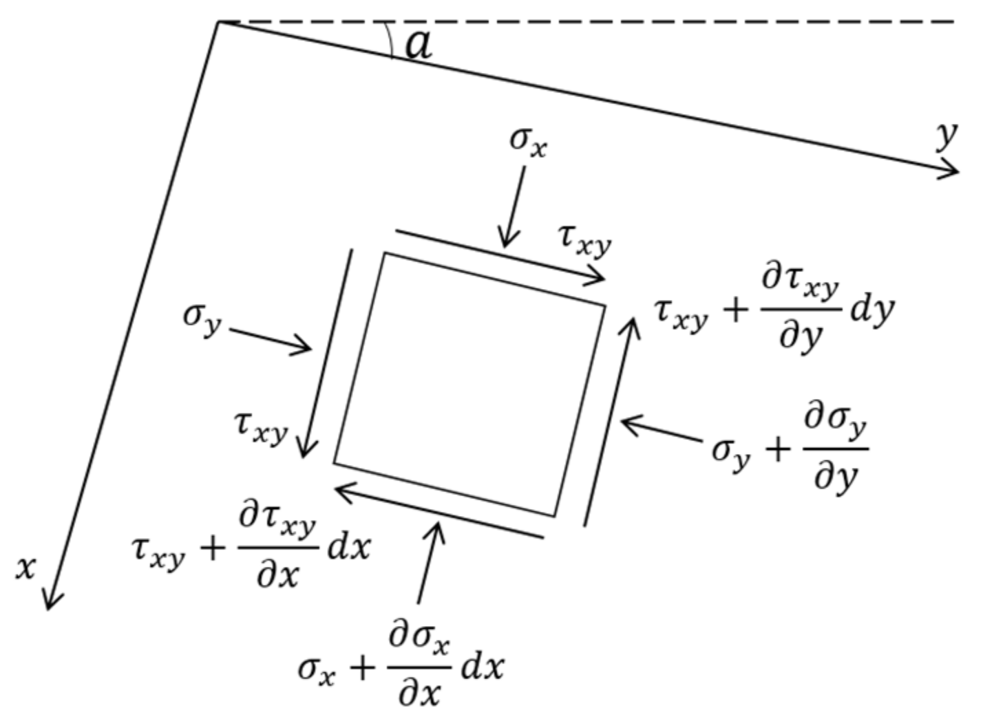
2.1. Application of Slip Line Method of Coulomb Material

To apply the slip line method, the following assumptions are made:

• The soil body is an ideal hard plastic body.
• Mohr–Coulomb yield criteria are followed.
• When a load is applied, the plastic area of the ground can move freely.
• The plastic deformation of the ground is large; therefore, elasticity can be neglected.

As shown in Figure 1, under the plane strain condition, a point on the plane always has principal stresses perpendicular to each other.

If the lines indicating the direction of the principal stress are continuously connected at each point, curves orthogonal to each other can be obtained. This line is called the principal stress trajectory, and there are two failure surfaces at each point, as shown in Figure 2b and Figure 3. By successively connecting the failure surfaces (or slip lines) of each point, two curves can be obtained, and the curves are called slip lines.

Figure 2a shows the slip line $\alpha$ and $\beta$ using Mohr circle in Coulomb material. In Figure 2a, $p$ is the average stress, and R is the radius of the stress circle. In Figure 2b, ${\sigma }_1$ is the maximum principal stress, and ${\sigma }_3$ is the minimum principal stress. $\alpha$, $\beta$ denote the slip line (shear failure surface), and $\mu$ is the angle between the maximum principal stress and the slip line (shear failure surface).

Figure 3 shows the principal stress trajectories and slip lines of the Coulomb material. Curves 1 and 2 are the principal stress trajectories, and $\theta$ is the angle between the maximum principal stress and the x-axis. Each point has two failure surfaces, as shown in Figure 2. Two slip lines can be obtained by continuously connecting the failure surfaces of each point. These slip lines are line $\mathsf{\alpha }$ and line $\mathsf{\beta }$ in Figure 3.

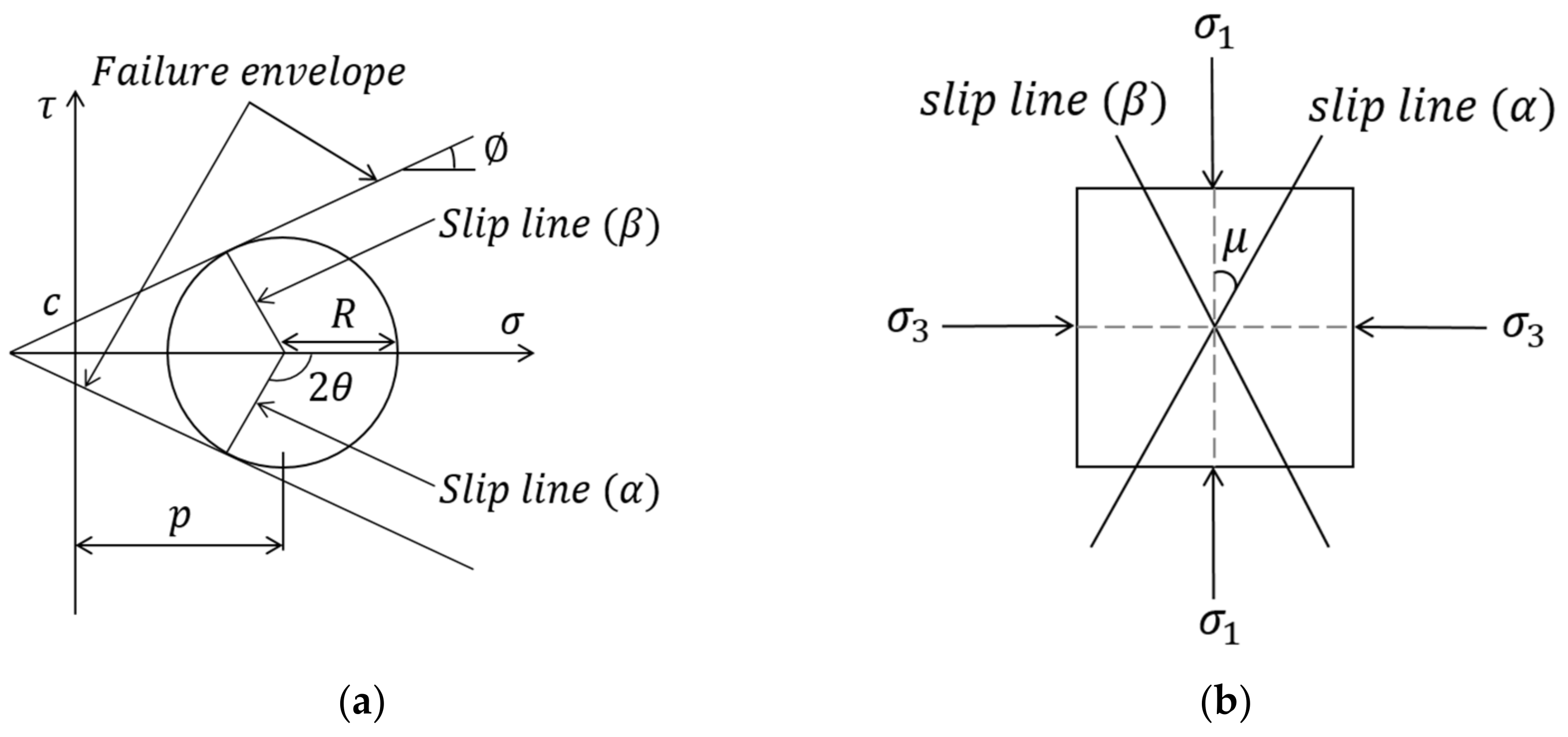
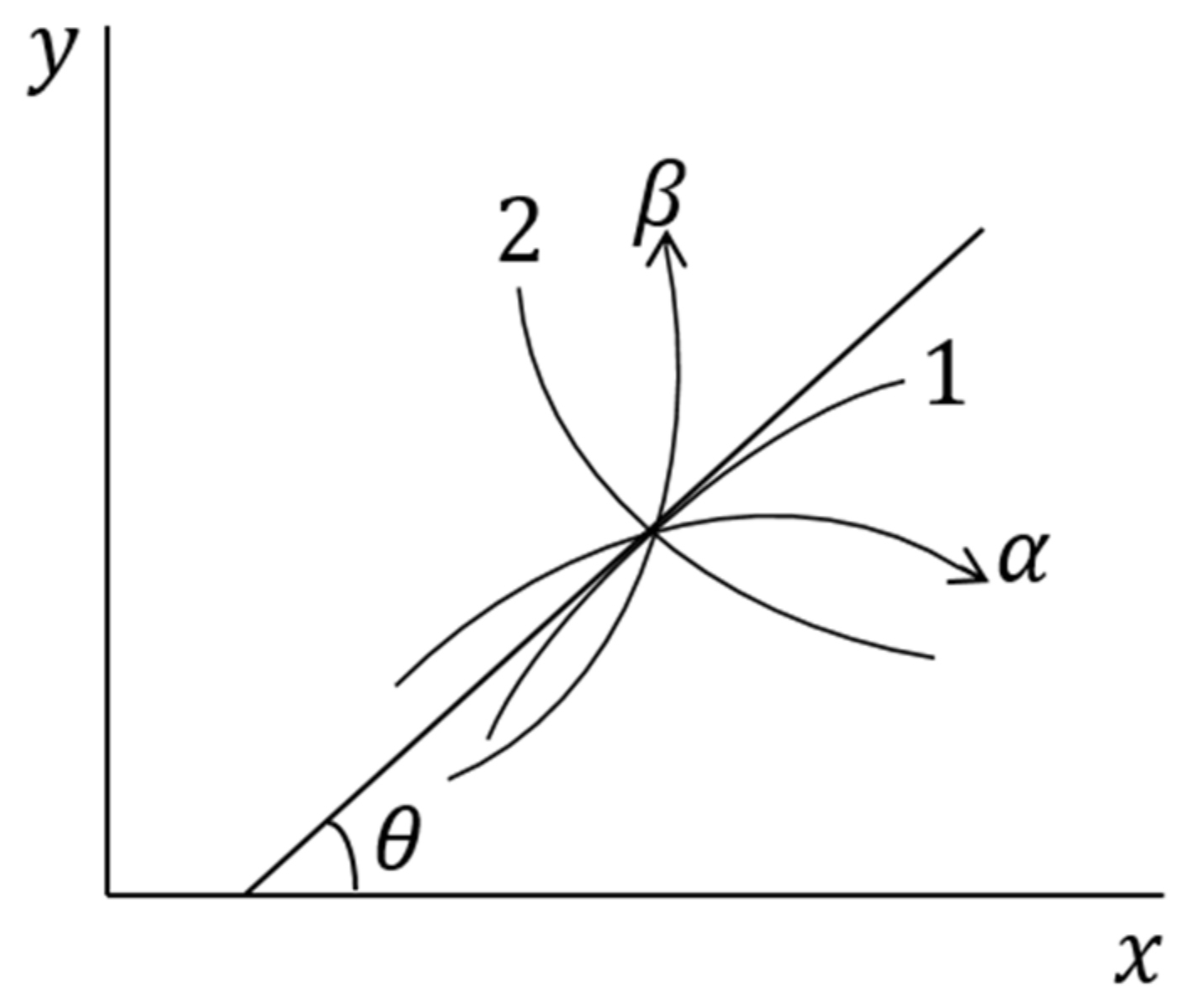
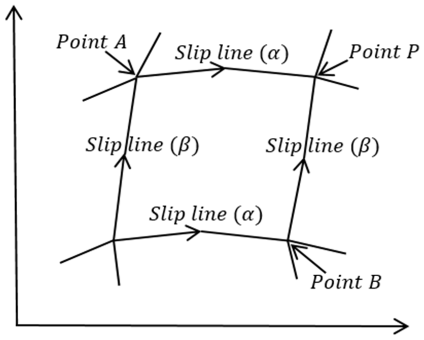
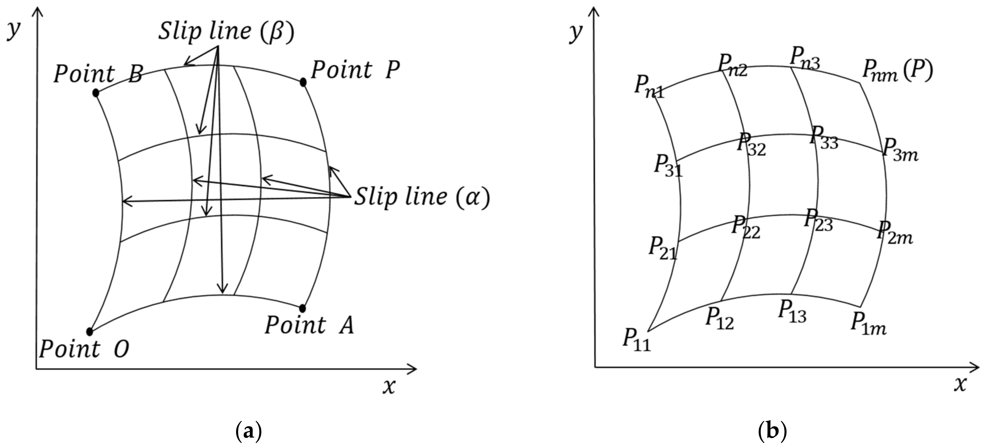
2.2. Recurrence Formula of the Slip Line Method

To solve various geotechnical problems by applying the numerical analysis method of the slip line method, three boundary problems (Cauchy, Riemann, mixed) and the basic calculation method are applied. The basic calculation method determines the intersection of the α line passing through point A and the β line passing through point B using the given average stress p and θ values at points A and B. Through this, the average stress p and θ values at point P can be obtained.

A limitation of the basic calculation method is that one cannot integrate along a characteristic line unless the positions of the $\alpha$ line through point A and the $\beta$ line through point B are known. Therefore, it is possible to obtain a solution by combining the stress equation and the slip line equation to obtain the position of the P point ($X_p$, $Y_p$) and ${\theta }_p$, $P_p$ as shown in Figure 4.

The recurrence formula can be derived from the stress equation (Equations (1) and (2)) derived from Figure 1 and the slip line equation (Equations (3) and (4)) derived from Figure 3. This is shown in Equations (5)–(8).

$$-sin2\mu \left(P_P-P_A\right)+\left(R_P+R_A\right)\left({\theta }_P-{\theta }_A\right)=-\mathsf{\gamma }sin\left(2\mu \right)\left(x_P-x_A\right)-\gamma cos\left(2\mu \right)\left(y_P-y_A\right)$$

(1)

$$sin2\mu \left(P_P-P_B\right)+\left(R_P+R_B\right)\left({\theta }_P-{\theta }_B\right)=\mathsf{\gamma }sin\left(2\mu \right)\left(x_P-x_B\right)-\gamma cos\left(2\mu \right)\left(y_P-y_B\right)$$

(2)

$$y_P-y_A=tan\left(\frac{{\theta }_P+{\theta }_A}{2}-\mu \right)\left(x_P-x_A\right)={(\frac{dy}{dx})}_1\left(x_P-x_A\right)$$

(3)

$$y_P-y_B=tan\left(\frac{{\theta }_P+{\theta }_B}{2}+\mu \right)\left(x_P-x_B\right)={(\frac{dy}{dx})}_2\left(x_P-x_B\right)$$

(4)

$${\theta }_p=\frac{\gamma sin2\mu \left(x_A-x_B\right)-\gamma cos2\mu \left(2y_P-y_A-y_B\right)+sin2\mu \left(P_B-P_A\right)+\left(R_P+R_A\right){\theta }_A+\left(R_P+R_B\right){\theta }_B}{\left(2R_P+R_A+R_B\right)}$$

(5)

$$P_P=\frac{\gamma sin2\mu \left(x_P-x_B\right)-\gamma cos2\mu \left(y_P-y_B\right)+P_{B}sin2\mu -\left({\theta }_P+{\theta }_{\mathrm{B}}\right)sin\varnothing -2\mathrm{c}\left({\theta }_P+{\theta }_B\right)cos\varnothing }{sin2\mu +sin\varnothing \left({\theta }_P-{\theta }_B\right)}$$

(6)

$$y_P=y_B+{\left(\frac{dy}{dx}\right)}_2·\left(x_P-x_B\right)$$

(7)

$$\begin{gathered} x_P\frac{\left(y_B-y_A\right)+{(\frac{dy}{dx})}_1 x_A-{(\frac{dy}{dx})}_2 x_B}{{\left(\frac{dy}{dx}\right)}_1-{\left(\frac{dy}{dx}\right)}_2} (\mathrm{When} \mathrm{two} \mathrm{points} \mathrm{are} \mathrm{known}) \\ {x}_P=x_A+\frac{y_P-y_A}{tan\left({\theta }_P+{\theta }_A/2-\mu \right)} \mathrm{or} x_P=x_B+\frac{y_P-y_B}{tan\left({\theta }_P+{\theta }_B/2-\mu \right)} (\mathrm{When} \mathrm{one} \mathrm{point} \mathrm{is} \mathrm{known}) \end{gathered}$$

(8)

In Equations (1), (2), (5), and (6), $\gamma$ means unit weight.

In this paper, the slip line method was applied to the slope. Therefore, if the $\theta$ and p values of two different pairs of slip lines are known, the plastic area can be analyzed by applying the Riemann problem, which can find a solution within the area of influence of the slip line. Figure 5a shows a schematic diagram of the Riemann boundary problem to be solved using the slip line method, where curves OA and OB are two different slip lines. The x, y, p, $\theta$ values of points $P_{12}$ and $P_{21}$ in Figure 5b can be calculated using the basic calculation method. The approximation of each point in the area of influence can be calculated in the same way ($P_{13}$, $P_{31,}$ etc.).

3. Analysis of Failure Area

The slip line method has the features of clearly presenting the failure area expressed using the Cartesian coordinate system by the recurrence formula derived based on the finite difference method and the stress value of the corresponding coordinate. For comparative verification of the failure area analyzed by the slip line method, the plastic area was analyzed through finite element limit analysis.

As a result of the analysis of the slip line method, the failure surface and internal stress can be presented regardless of conditions such as the low slope of the ground or high ground strength.

These results are explained by lower-bound analysis. The stress–strain relationship of limit analysis is the same as that of the perfect-strain model.

The perfect-strain model is a model in which yielding and failure occur at the same time according to stress. The lower-limit analysis is a method of analyzing with a stress field in the elastic region before stress yielding occurs, and the upper-limit analysis is a method of analyzing with a velocity field using the rate of strain in the region where stress failure occurs. It is shown in Figure 6.

The limit analysis is a method to obtain a mathematical solution by simultaneously performing the upper- and lower-limit analysis. Our study does not provide a mathematical solution; however, through the features of the lower-limit analysis, the failure area and the stable area are distinguished; the failure area in the heterogeneous ground is presented.

Using this principle, the slip line method can distinguish the plastic deformation area and the no deformation area, as shown in Figure 7.

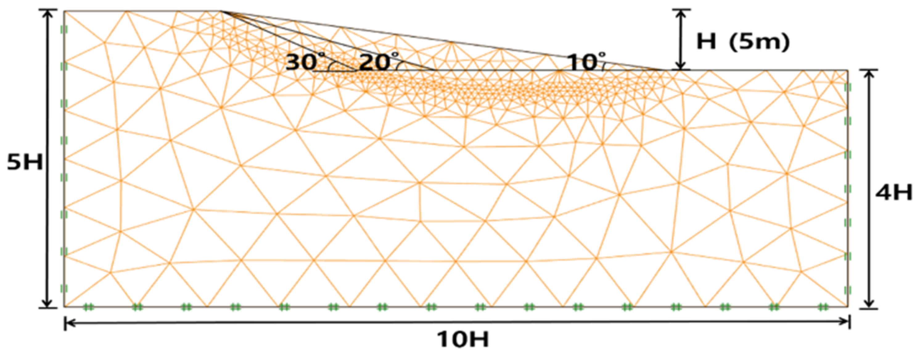
3.1. Analysis Condition of Slope Failure Area

For the analysis of the failure area of a heterogeneous ground slope using the slip line method, the ground consists of soft ground (alluvium, sedimentary) and hard ground (weathered rock, soft rock); the physical properties of the ground are shown in

Table 1. Geomechanical characteristics of simulated ground [29].

Ground Property	Alluvium	Sedimentary Soil	Weathered Rock	Soft Rock
Cohesion (c, kPa)	15	17.5	50	100
Unit Weight ($\gamma , \mathrm{kN}/{\mathrm{m}}^3$)	17	18.5	21	24
Inner friction angle ($\varnothing , °)$	20	31	33	35.5

.

In this paper, to emphasize the features of the slip line method that can analyze the failure area under any conditions, the conditions in which it is difficult for failure to occur were set as follows.

The slope angle was very gentle (10°, 20°, 30°), and only self-weight was considered without external load. Failure begins with stress singularity. However, there is no stress singularity when eliminating external loads to analyze the failure area under conditions where it is difficult failure for to occur. Therefore, a virtual stress singular point was arbitrarily assumed at 4 m to the left of the starting point of the slope so that the failure area could be analyzed.

In this paper, the load condition was not set; therefore, the failure was induced through the strength reduction method. In addition, the strength reduction method does not assume the location of the critical failure surface, and there is no need to divide the slope at the critical failure surface into intercepts. Since the strength reduction method shares these features with the slip line method, it is expected that the difference in the analysis of the failure area could be compared; therefore, it was used as a comparison target.

As an analysis condition of the strength reduction method, a mesh was created with very fine triangular elements, and the boundary conditions were set as lower hinges (vertical and horizontal fixed); left and right rollers (horizontal fixed) as shown in Figure 8.

In this study, for the analysis of the slip line method, a virtual slope was analyzed rather than an actual slope. Due to the limitations of the Riemann boundary problem that was applied to analyze the failure area of the slope, the analysis conditions were set as follows.

The initial boundary condition consisted of flat ground and slopes, no external load (p = 0) was assumed, the θ value was set arbitrarily, and the convergence value of θ was presented through a recurrence formula.

Moreover, to analyze the failure area of the heterogeneous ground slope, the slope was divided into upper and lower ground, and the slope angle was expressed as δ ($10°$, $20°$, $30°$). The upper ground of the slope was set at 1.5 m, and the lower ground varied based on the failure analysis. This is shown in Figure 9.

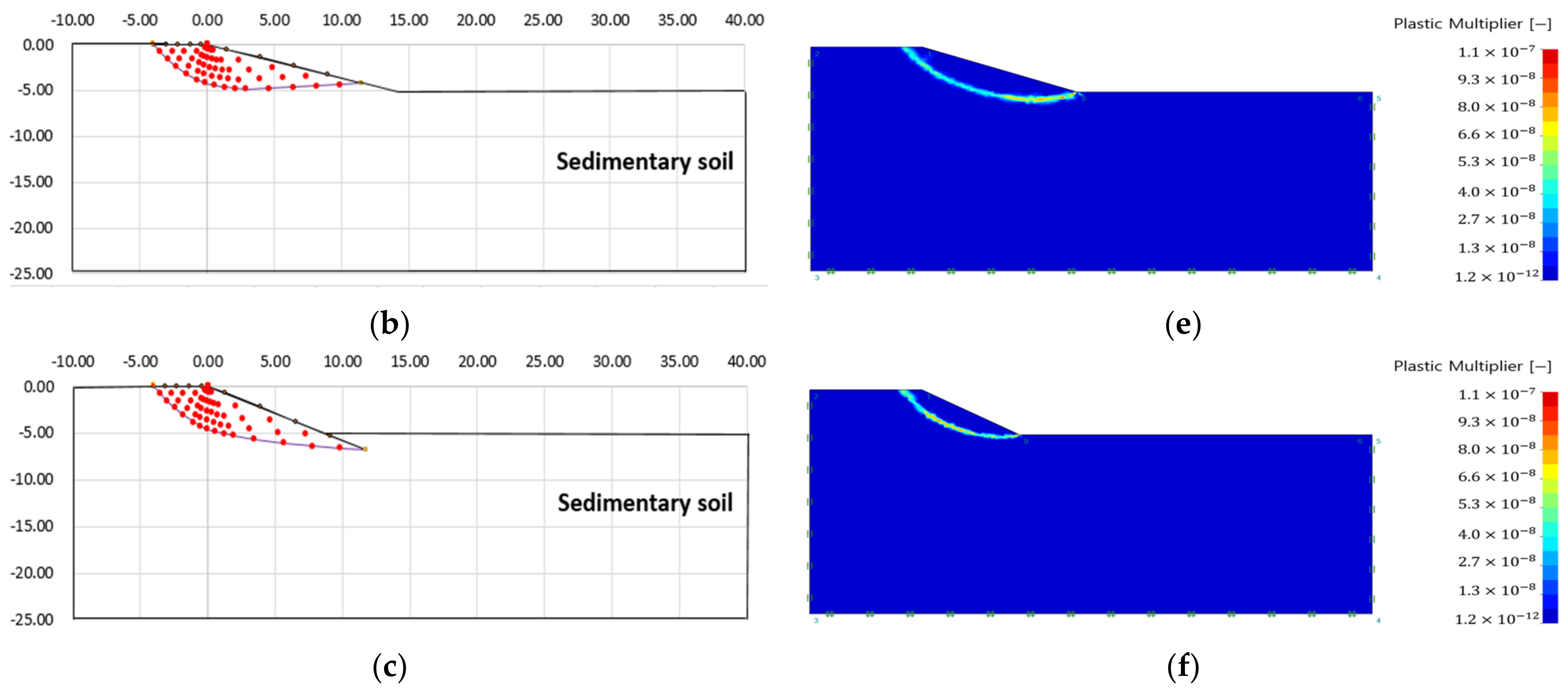
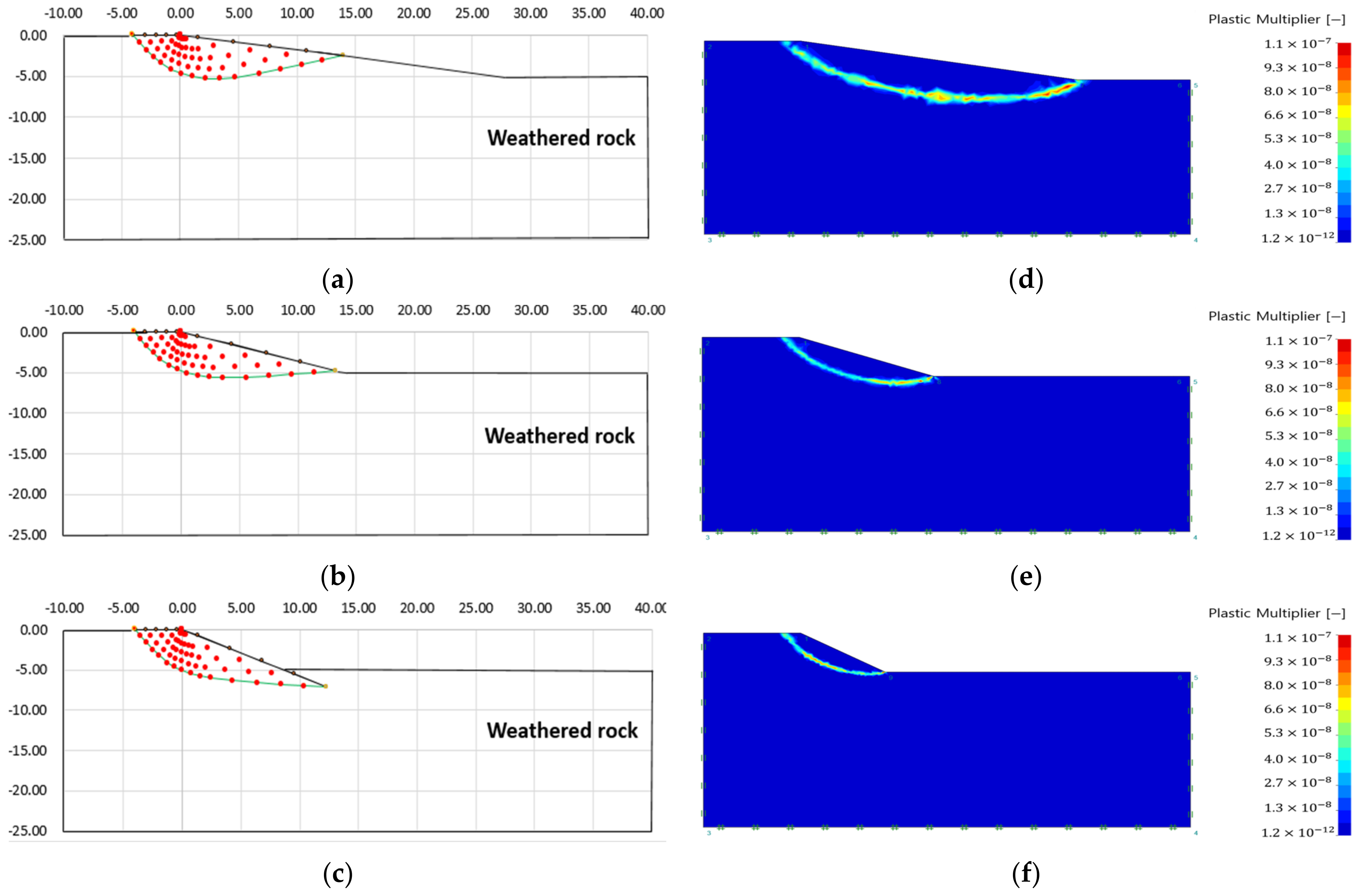
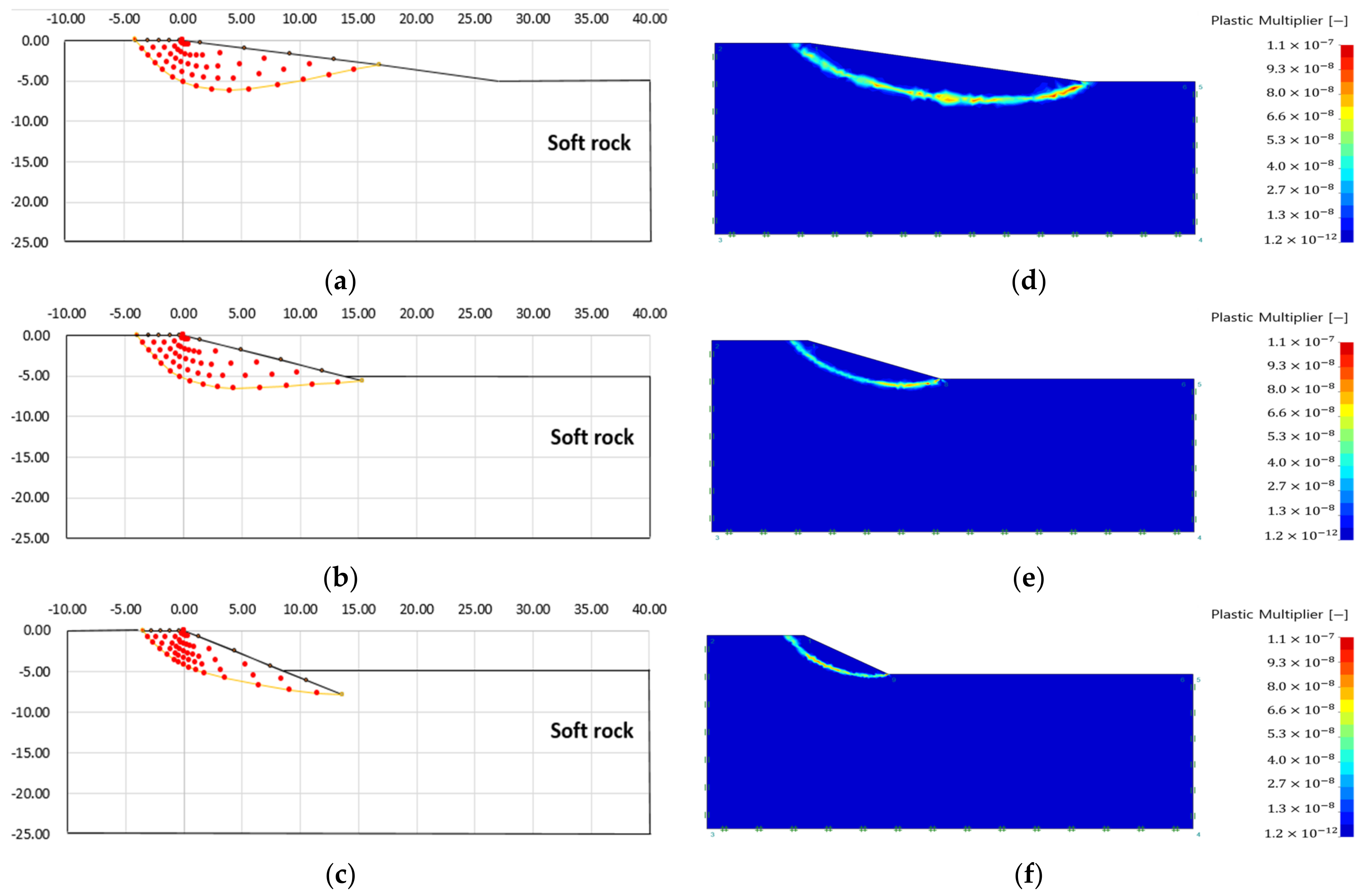
3.2. Analysis of the Failure Area of a Single Ground Slope

Figure 10, Figure 11, Figure 12 and Figure 13 show the failure area using the slip line method and the strength reduction method according to the analysis conditions of a single ground.

Table 2. Analysis result of failure area of single ground analyzed by slip line method.

	Ground	Alluvium			Sedimentary Soil			Weathered Rock			Soft Rock
Property
Slope angle ($°$)		10	20	30	10	20	30	10	20	30	10	20	30
Failure area depth (m)		3.36	3.81	7.36	4.46	4.83	6.76	5.31	5.59	7.06	6.17	6.5	7.86
Failure area length (m)		7.25	8.18	12.8	11.4	11.5	11.7	13.9	13.2	12.2	16.8	15.4	13.6
Maximum internal stress (kPa)		296.16	203.19	130.36	1038.51	677.26	401.20	2200.07	1478.94	952.53	4476.83	3016.08	1985.89

shows the failure area scale and internal stress analysis results of a single ground.

As a result of the slip line method, the depth of the failure area increases as the slope increases (see Figure 10, Figure 11, Figure 12 and Figure 13, Table 2). The maximum internal stress appears at the point where the virtual failure surface begins (virtual singularity), decreases as the slope increases, and increases as the ground strength increases (see Table 2).

As a result of the finite element limit analysis, the plastic area was analyzed as larger than the slip line method in all analysis conditions, and there was no significant difference in the scale of the plastic area according to the ground properties. It can be seen that the plastic area is formed at the start and end points of the slope, which are the stress singularity points.

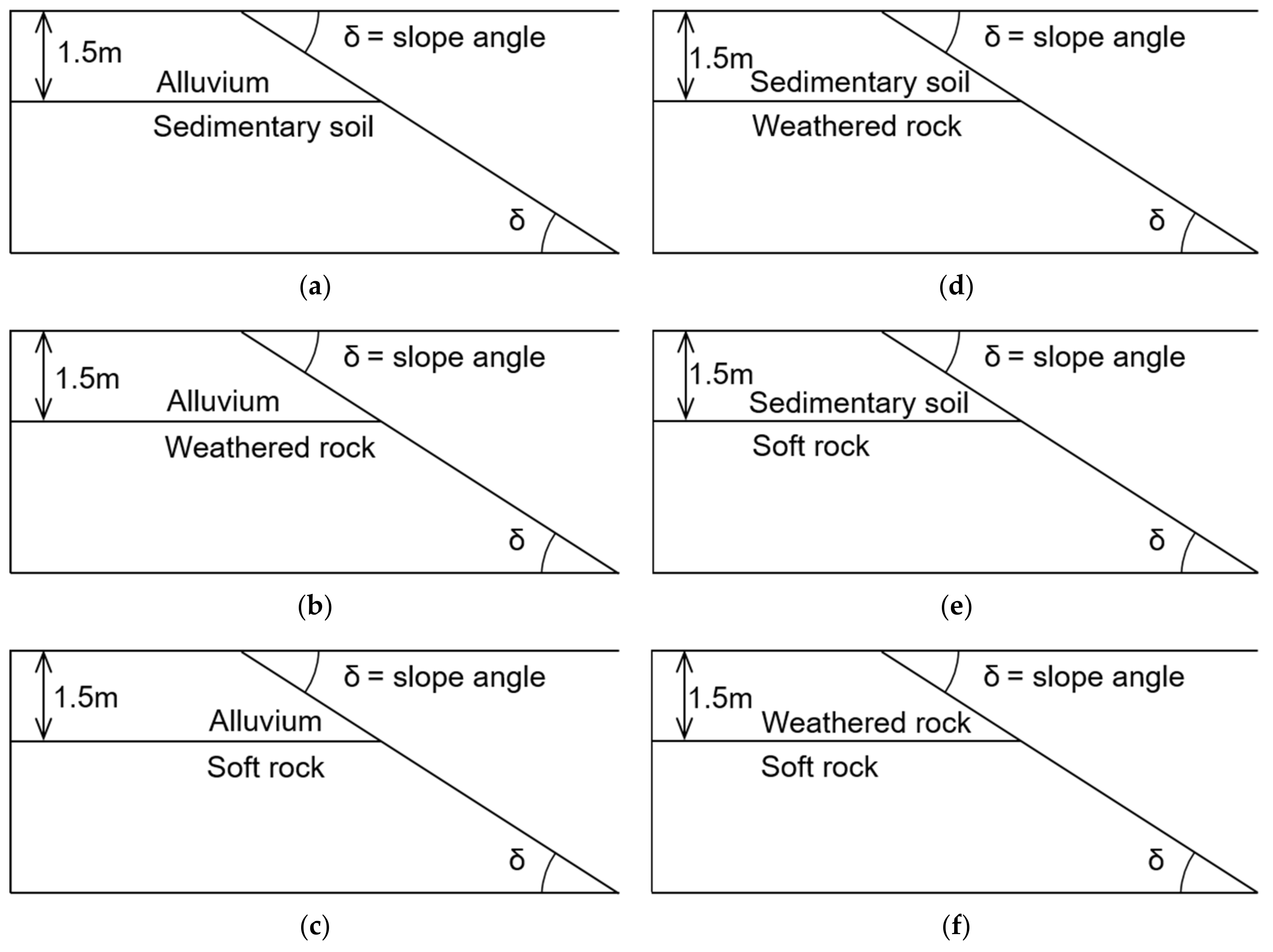
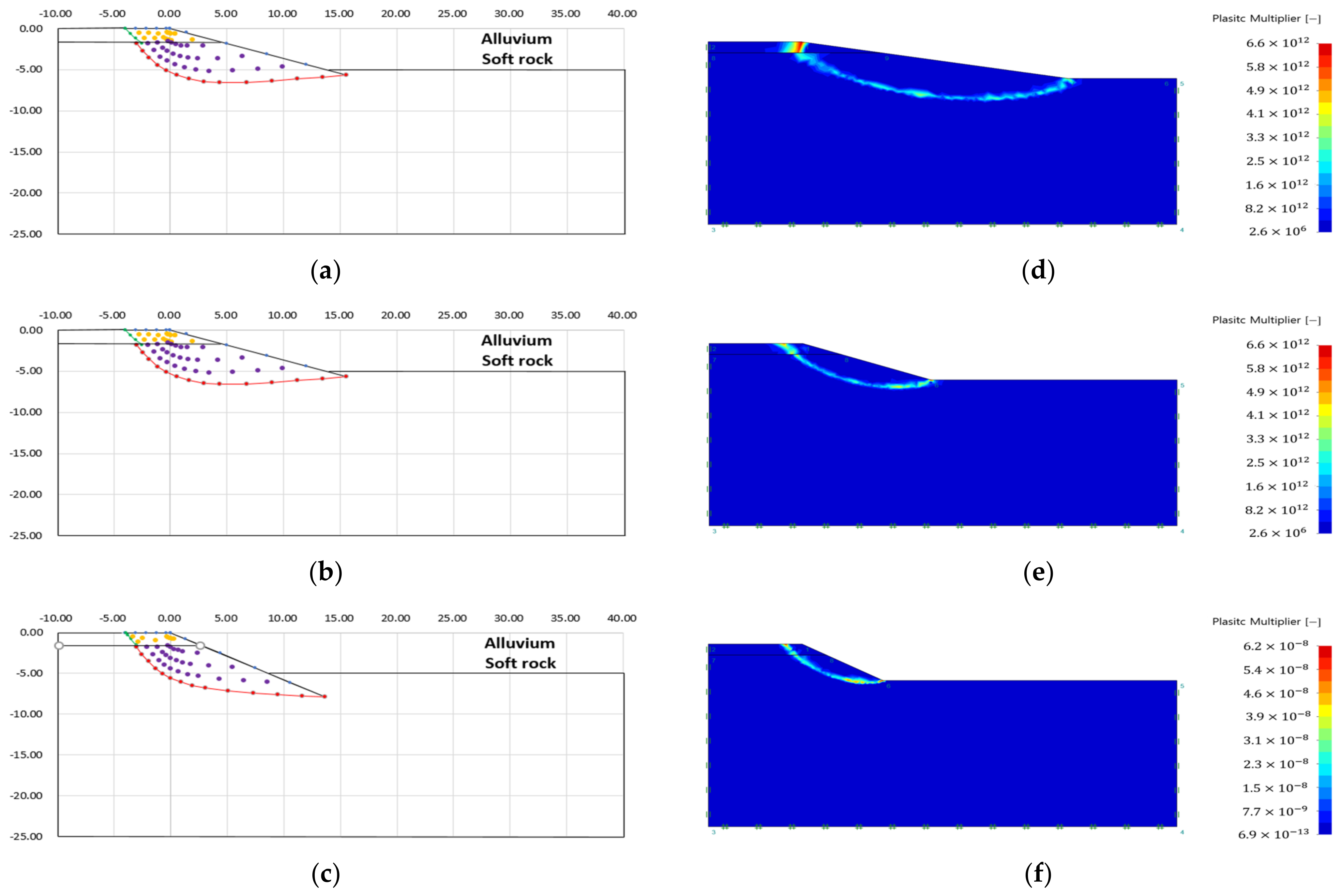
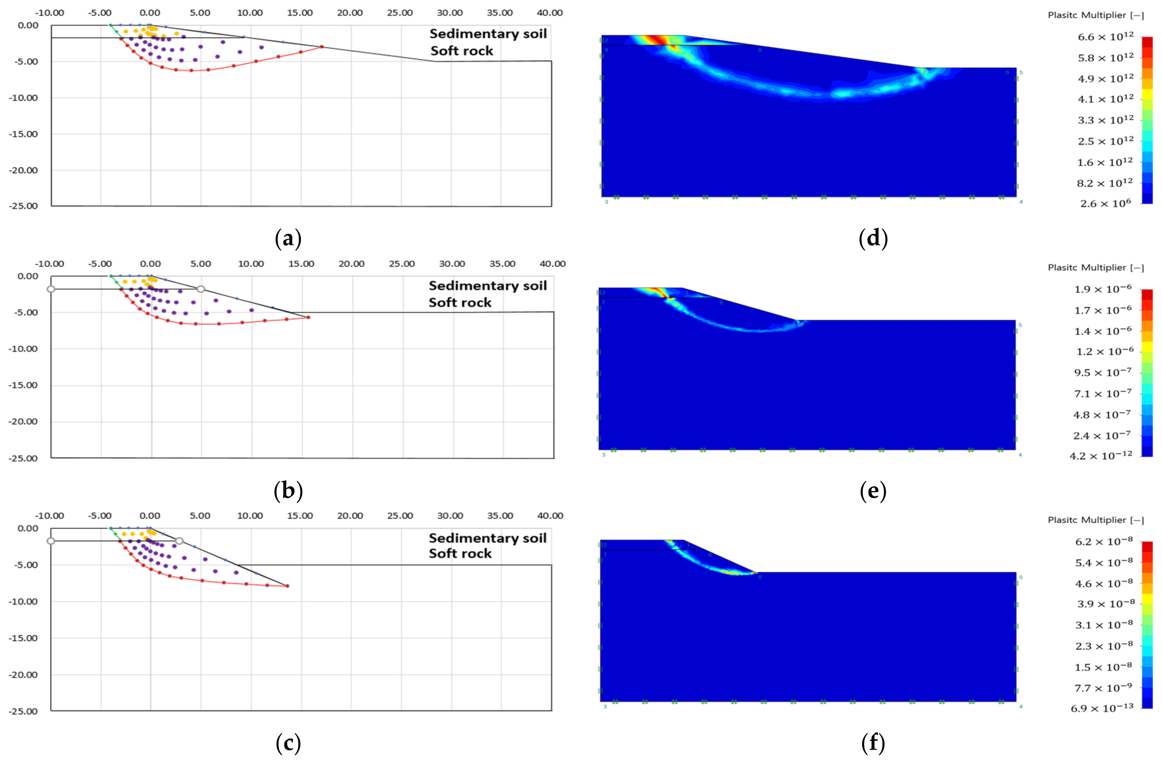
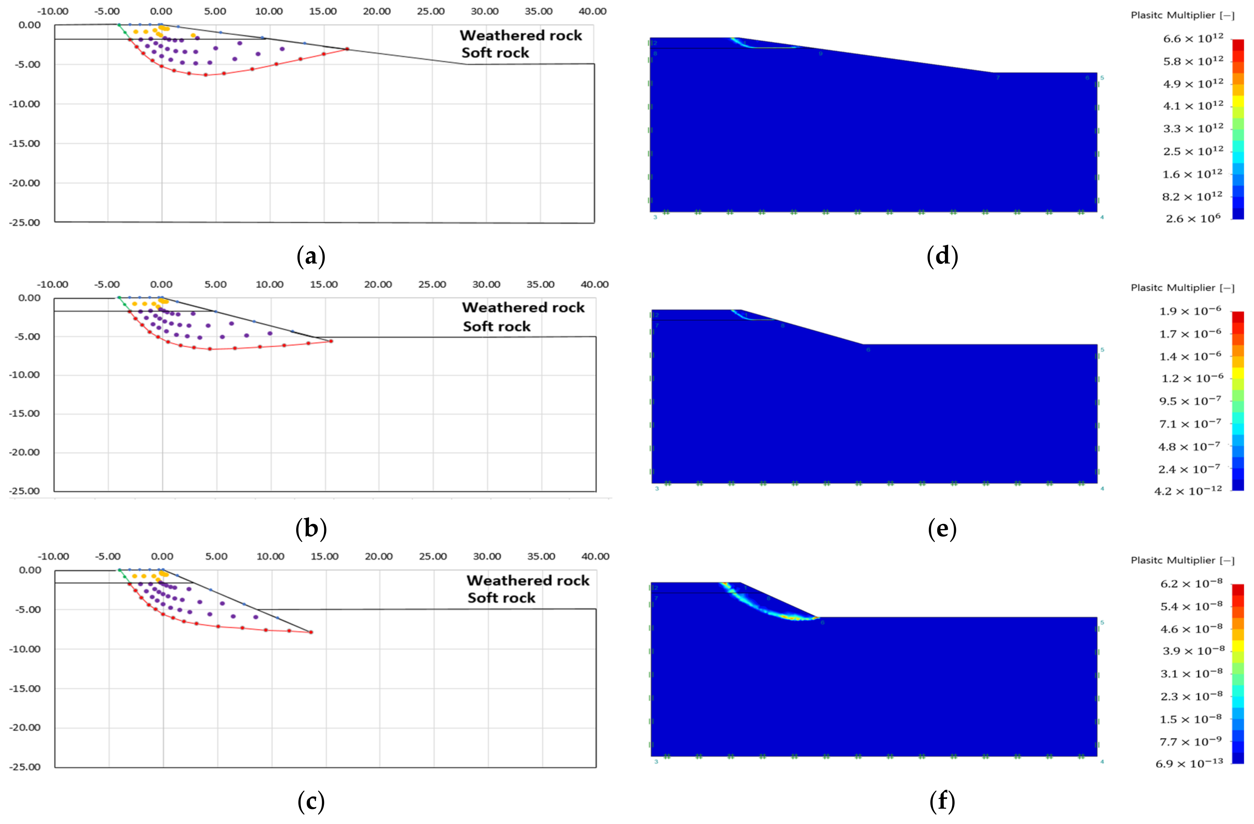
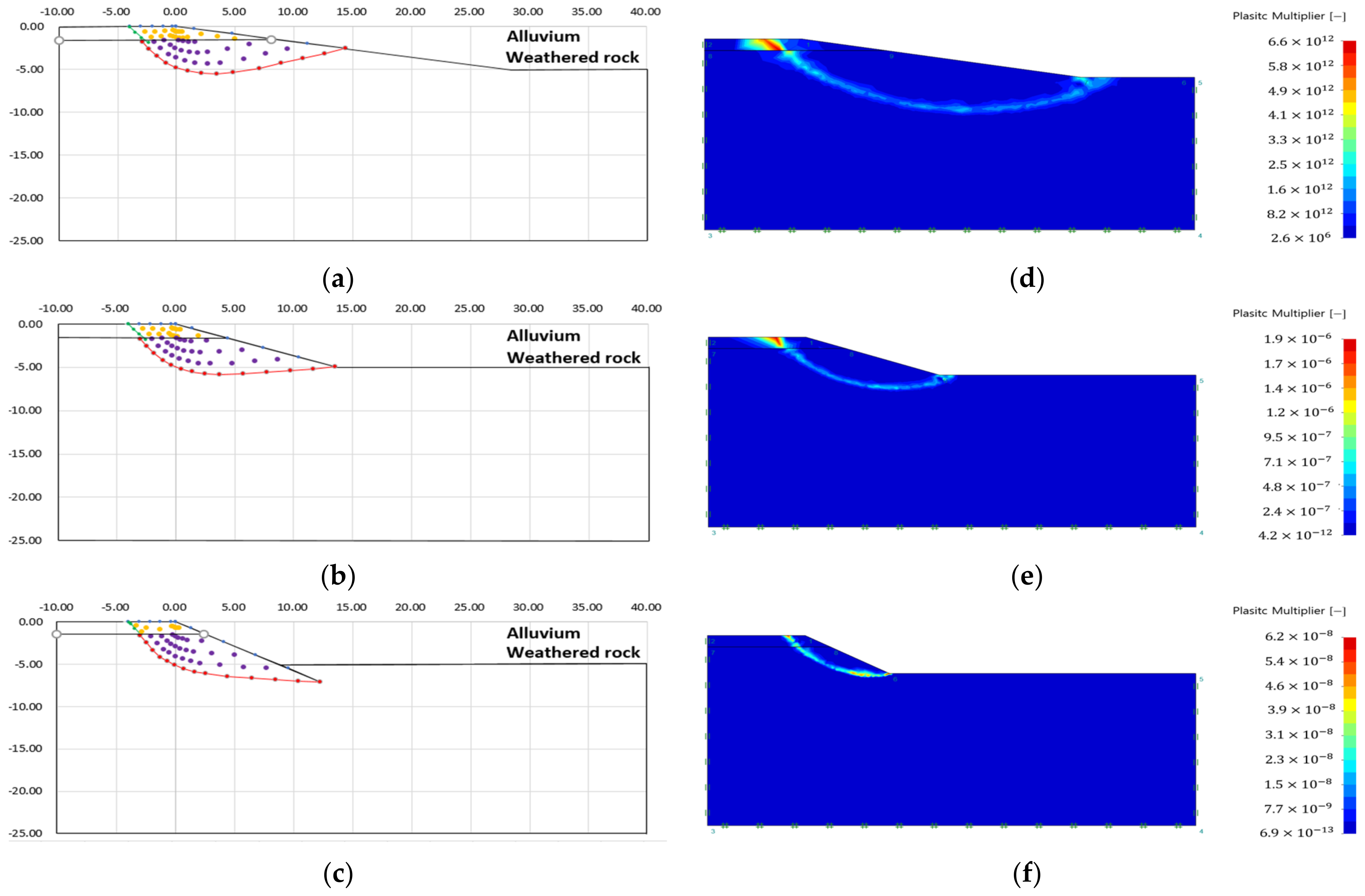
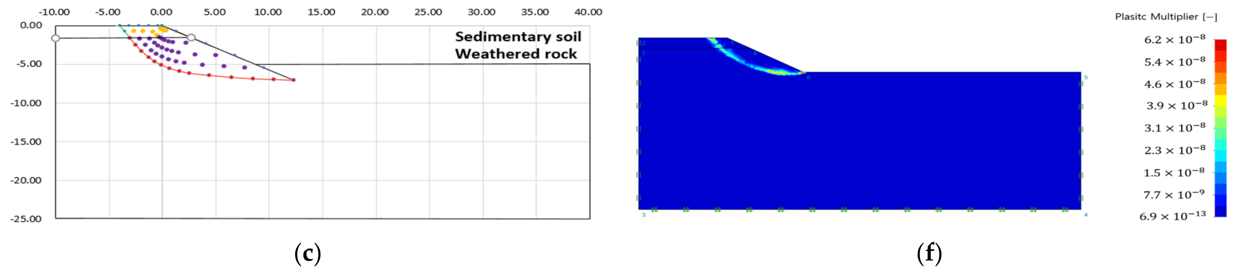
3.3. Analysis of Failure Area of Heterogeneous Ground Slope

Figure 14, Figure 15, Figure 16, Figure 17, Figure 18 and Figure 19 show the failure area using the slip line method and the strength reduction method according to the analysis conditions of the heterogeneous ground.

Table 3. Analysis result of plastic area of heterogeneous ground analyzed by slip line method.

	Ground	Case 1			Case 2			Case 3			Case 4			Case 5			Case 5
Property
Slope angle ($°$)		10	20	30	10	20	30	10	20	30	10	20	30	10	20	30	10	20	30
Failure area depth (m)		6.29	6.6	7.89	6.29	6.62	7.90	6.3	6.63	7.90	5.77	5.18	6.60	5.51	5.85	7.08	5.53	5.85	7.08
Failure area length (m)		17.1	15.6	13.7	17.1	15.6	13.7	17.2	15.6	13.7	14.7	11.9	11.4	14.4	13.5	12.3	14.5	13.5	12.3
Maximum internal stress (kPa)		4967.76	3386.2	2267.53	5007.52	3420.49	2292.87	5078.84	3472.64	2333.81	2910.29	936.70	605.46	2587.84	1776.37	1183.25	2621.87	1801.17	1203.34

shows the scale of the failure area and the results of the internal stress analysis according to the heterogeneous ground.

As a result of the failure area analysis, both analysis methods confirmed that the shape of the failure surface was discontinuously connected at the boundary of the heterogeneous layer (see Figure 14, Figure 15, Figure 16, Figure 17, Figure 18 and Figure 19). This is because of the difference in ground properties between the upper and lower ground.

The features revealed in the analysis results of the slip line method are as follows:

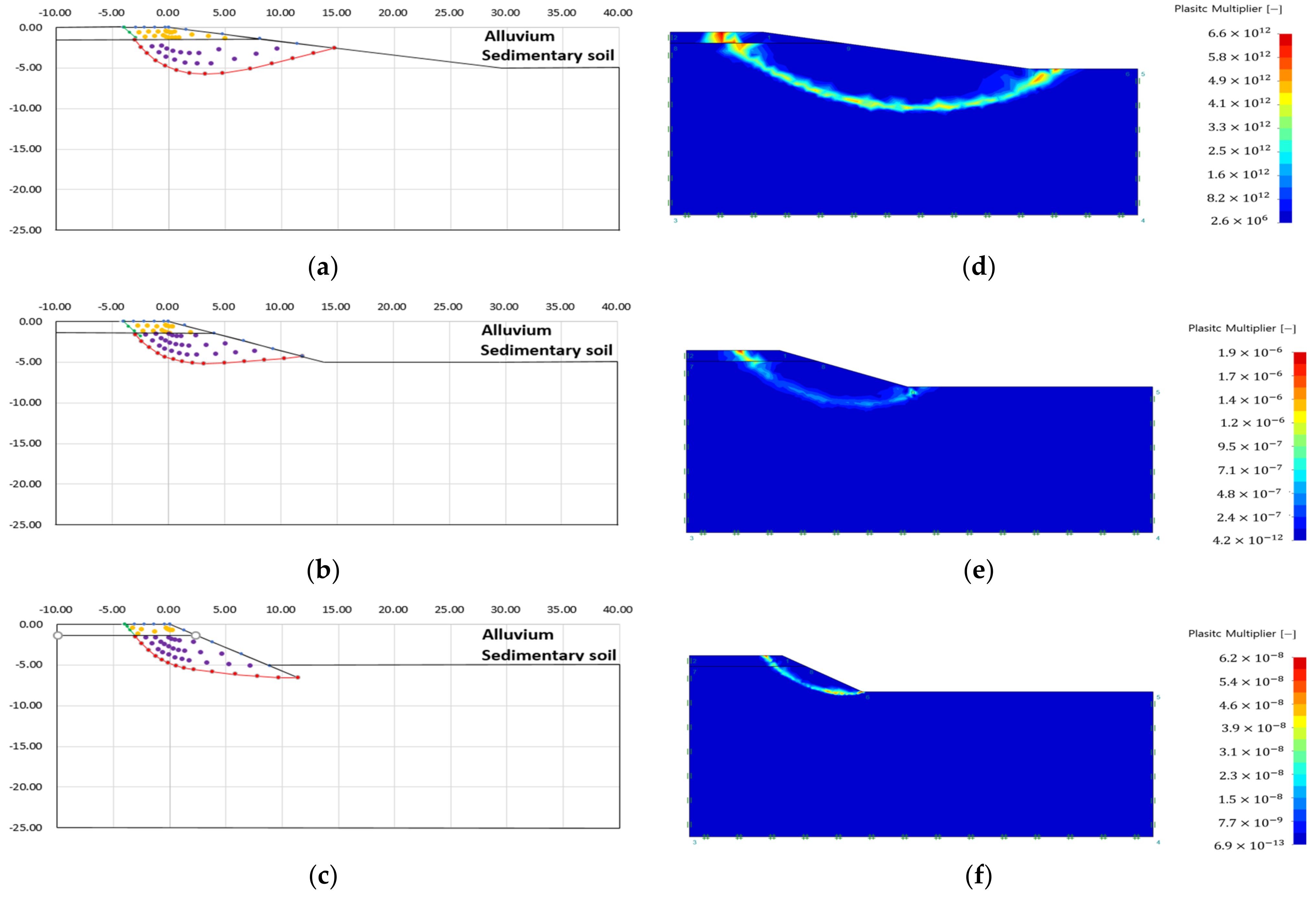
• The failure surface of the upper and lower ground changed according to the internal friction angle of each ground. The green line is the failure surface according to the internal friction angle of the upper ground, and the red line is the failure surface according to the internal friction angle of the lower ground.
• There was no significant difference in the failure area, because there is small variation in the internal friction angle according to each analysis condition. However, it could be confirmed that the difference in internal stress was different because of the difference in other ground properties (cohesion, unit weight) (see Table 3).

The features revealed in the analysis of the finite element limit analysis are as follows:

3.

The plastic area appeared over the entire slope when the difference in ground properties between the upper and lower ground was small, or the slope angle was large.

4.

Case 1, in which the difference in ground properties between the upper and lower ground was the largest, showed a plastic area limited to the upper ground. This is because the upper ground, which had the lowest ground properties, failed before the lower ground, because the strength reduction method was applied without external load.

5.

As with the analysis result of the single ground, there was no stress singularity, such as an external load. Therefore, the failure area was formed at the start and end points of the slope, which were the other stress singular points.

6.

As with the analysis results of the slip line method, it can be seen that the failure surface was discontinuously connected to the ground boundary layer.

4. Conclusions

This study conducted failure behavior analyses of single ground and heterogeneous ground slopes using the slip line method. The analysis results through the slip line method and the strength reduction method of the finite element analysis were compared, and the following conclusions were drawn.

• The slip line method showed a clear virtual failure surface regardless of the ground strength and slope. In addition, it is possible to calculate the internal stress of the coordinates according to the coordinates (x, y) expressed in the Cartesian coordinate system.
• In the case of finite element limit analysis, the plastic area analyzed by the strength reduction method was similar to the analysis result of the slip line method. However, it should be noted that the strength reduction method reduces the strength of the entire ground properties. Therefore, the plastic area was over-analyzed because the analysis was performed using the strength reduction method in the absence of stress singularities such as load.
• As a result of analyzing the failure area of a single ground, the slip line method increased the scale of the failure surface as the slope of the soft ground (alluvium, sedimentary layer) increased. In the case of finite element limit analysis, it was confirmed that there was no significant difference in the plastic region depending on the properties of the ground and the slope angle.
• As a result of the analysis of the failure area of the heterogeneous ground, the slip line method showed that the shape of the failure surface changed according to the change of the ground characteristic value, and the failure area and the virtual failure surface were clearly expressed regardless of the ground condition and slope angle. In addition, in the case of heterogeneous ground, the upper ground was regarded as a surcharge load and applied to the lower ground for analysis, showing a difference from the analysis results of a single ground.
• In the case of finite element limit analysis, it can be seen that the failure surface is discontinuously connected to the ground boundary layer. In addition, when the difference in soil properties between the upper ground and the lower ground was the greatest, the failure area was limited to the upper ground. This is because the upper ground with the lowest ground properties failed before the lower ground because the strength reduction method was applied without external load. It should be noted that the plastic area was over-analyzed by considering the shape of the slope as a stress singular point, because the analysis was performed using the strength reduction method in the absence of stress singularity such as load.
• The slip line method analyzes the plastic area based on boundary conditions. Since the Riemann problem applied to the slope analysis sets the slip line as the boundary condition, the boundary condition can change. Because of these features, there is a risk that the plastic area and failure surface may be analyzed to be larger than the shape of the slope. Therefore, it is thought that a combination of boundary conditions according to the structure or geotechnical problem is necessary.
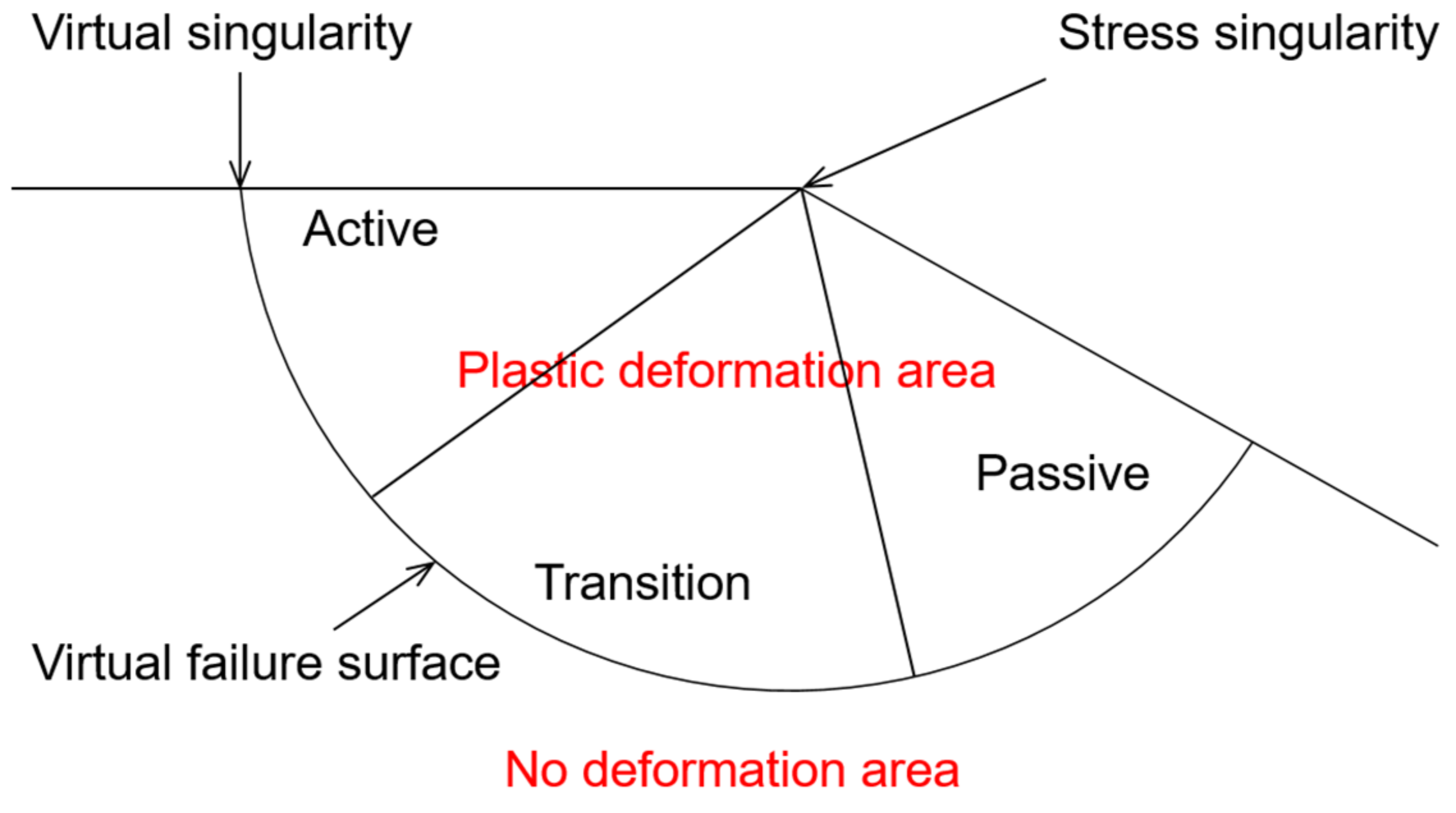
• The slip line method can determine the virtual failure surface, failure area (active area, transition area, passive area), and internal stress if only the basic boundary conditions and ground characteristics are given. In addition, in this paper, it was shown that analysis of heterogeneous ground is possible. Through these features, the applicability and development potential of the slip line method to various geotechnical problems or structures were confirmed.

References

1. Bolton, H.; Heymann, G.; Groenwold, A. Global search for critical failure surface in slope stability analysis. Eng. Optim. 2003, 35, 51–65. [Google Scholar] [CrossRef]
2. Cheng, Y. Location of critical failure surface and some further studies on slope stability analysis. Comput. Geotech. 2003, 30, 255–267. [Google Scholar] [CrossRef]
3. Cheng, Y.; Li, L.; Chi, S.-C.; Wei, W. Particle swarm optimization algorithm for the location of the critical non-circular failure surface in two-dimensional slope stability analysis. Comput. Geotech. 2007, 34, 92–103. [Google Scholar] [CrossRef]
4. Kahatadeniya, K.; Nanakorn, P.; Neaupane, K. Determination of the critical failure surface for slope stability analysis using ant colony optimization. Eng. Geol. 2009, 108, 133–141. [Google Scholar] [CrossRef]
5. Himanshu, N.; Kumar, V.; Burman, A.; Maity, D.; Gordan, B. Grey wolf optimization approach for searching critical failure surface in soil slopes. Eng. Comput. 2020, 37, 2059–2072. [Google Scholar] [CrossRef]
6. Khajehzadeh, M.; Keawsawasvong, S.; Sarir, P.; Khailany, D.K. Seismic Analysis of Earth Slope Using a Novel Sequential Hybrid Optimization Algorithm. Period. Polytech. Civ. Eng. 2022, 66, 355–366. [Google Scholar] [CrossRef]
7. Zolfaghari, A.R.; Heath, A.C.; McCombie, P.F. Simple genetic algorithm search for critical non-circular failure surface in slope stability analysis. Comput. Geotech. 2005, 32, 139–152. [Google Scholar] [CrossRef]
8. Li, S.; Shangguan, Z.; Duan, H.; Liu, Y.; Luan, M. Searching for critical failure surface in slope stability analysis by using hybrid genetic algorithm. Géoméch. Eng. 2009, 1, 85–96. [Google Scholar] [CrossRef]
9. Sengupta, A.; Upadhyay, A. Locating the critical failure surface in a slope stability analysis by genetic algorithm. Appl. Soft Comput. 2009, 9, 387–392. [Google Scholar] [CrossRef]
10. Zhang, T.; Zhang, J.-Z. Numerical estimate of critical failure surface of slope by ordinary state-based peridynamic plastic model. Eng. Fail. Anal. 2022, 140, 106556. [Google Scholar] [CrossRef]
11. Li, W.; Zhang, C.; Zhang, D.; Ye, Z.; Tan, Z. Face stability of shield tunnels considering a kinematically admissible velocity field of soil arching. J. Rock Mech. Geotech. Eng. 2022, 14, 505–526. [Google Scholar] [CrossRef]
12. Zhang, C.; Han, K.; Zhang, D. Face stability analysis of shallow circular tunnels in cohesive–frictional soils. Tunn. Undergr. Space Technol. 2015, 50, 345–357. [Google Scholar] [CrossRef]
13. Tu, S.; Li, W.; Zhang, C.; Chen, W. Effect of inclined layered soils on face stability in shield tunneling based on limit analysis. Tunn. Undergr. Space Technol. 2023, 131, 104773. [Google Scholar] [CrossRef]
14. Shiau, J.; Lai, V.Q.; Keawsawasvong, S. Multivariate adaptive regression splines analysis for 3D slope stability in anisotropic and heterogenous clay. J. Rock Mech. Geotech. Eng. 2022. [Google Scholar] [CrossRef]
15. Yodsomjai, W.; Keawsawasvong, S.; Thongchom, C.; Lawongkerd, J. Undrained stability of unsupported conical slopes in two-layered clays. Innov. Infrastruct. Solutions 2020, 6, 15. [Google Scholar] [CrossRef]
16. Yodsomjai, W.; Keawsawasvong, S.; Likitlersuang, S. Stability of Unsupported Conical Slopes in Hoek-Brown Rock Masses. Transp. Infrastruct. Geotechnol. 2020, 8, 279–295. [Google Scholar] [CrossRef]
17. Lai, V.Q.; Lai, F.; Yang, D.; Shiau, J.; Yodsomjai, W.; Keawsawasvong, S. Determining Seismic Bearing Capacity of Footings Embedded in Cohesive Soil Slopes Using Multivariate Adaptive Regression Splines. Int. J. Geosynth. Ground Eng. 2022, 8, 46. [Google Scholar] [CrossRef]
18. Martin, C.M. User Guide for ABC—Analysis of Bearing Capacity (Version 1.0); OUEL Report No. 2261/03; University of Oxford: Oxford, UK, 2003. [Google Scholar]
19. Gao, F.-P.; Wang, N.; Zhao, B. A general slip-line field solution for the ultimate bearing capacity of a pipeline on drained soils. Ocean Eng. 2015, 104, 405–413. [Google Scholar] [CrossRef] [Green Version]
20. Liu, D.; Chen, X. Shearing characteristics of slip zone soils and strain localization analysis of a landslide. Géoméch. Eng. 2015, 8, 33–52. [Google Scholar] [CrossRef]
21. Keshavarz, A.; Fazeli, A.; Sadeghi, S. Seismic bearing capacity of strip footings on rock masses using the Hoek–Brown failure criterion. J. Rock Mech. Geotech. Eng. 2016, 8, 170–177. [Google Scholar] [CrossRef]
22. Zhou, A.; Li, C.; Jiang, P.; Yao, K.; Li, N.; Wang, W. Slip Line Theory Based Stability Analysis on the Influence of Deep Excavation on Adjacent Slope. Math. Probl. Eng. 2018, 2018, 2041712. [Google Scholar] [CrossRef]
23. Tsegaya, A.B. Bearing capacity of shallow foundations that are situated at a varying distance from slopes. In Proceedings of the XVII European Conference ESCMGE-2019, Reykjavik, Iceland, 1–6 September 2019. [Google Scholar]
24. Park, S.Y.; Han, H.S. Earth Pressure Analysis of Tunnel Ceiling according to Tunnel Plastic Zone. J. Korea Acad. -Ind. Coop. Soc. 2020, 21, 753–764. [Google Scholar] [CrossRef]
25. Lee, Y.K. Calculation of Failure Load of V-shaped Rock Notch Using Slip-line Method. Tunn. Undergr. Space 2020, 30, 404–416. [Google Scholar] [CrossRef]
26. Hill, R. The Mathematical Theory of Plasticity; Clarendon Press & Oxford: Oxford, UK, 1950. [Google Scholar]
27. Sokolovskii, V.V.; Kushner, J.K. Statics of Granular Media. J. Appl. Mech. 1966, 33, 239. [Google Scholar] [CrossRef] [Green Version]
28. Wang, R.; Skirrow, R.K.; Jianping, S. Slip line soiltion by spreadsheet. In Proceedings of the GeoEdmonton’08: 61st Canadian Geotechnical Conference and 9th Joint CGS/IAH-CNC Groundwater Conference, Edmonton, AB, Canada, 21–24 September 2008. [Google Scholar]
29. Soilworks. SoilWorks Ground Property Database. MIDAS IT Co., Ltd., 2022. Available online: https://www.midasuser.com (accessed on 12 July 2022).
Figure 1. Coordinate plane for plane strain problem [27].
Applsci 13 03863 g001
Figure 2. Mohr circle notation of plastic stress state of Coulomb material [27]. (a) Slip line represented by Mohr circle; (b) stress state at a point.
Applsci 13 03863 g002
Figure 3. Principal stress trajectory and slip lines for coulomb material [27].
Applsci 13 03863 g003
Figure 4. Basic calculation method [27].
Applsci 13 03863 g004
Figure 5. Numerical analysis method of Riemann problem [27]; (a) Riemann problem basic assumptions; (b) Numerical analysis process.
Applsci 13 03863 g005
Figure 6. Schematic diagram of limit analysis applied to plastic area analysis.
Applsci 13 03863 g006
Figure 7. Schematic diagram of plastic area analysis using the slip line method.
Applsci 13 03863 g007
Figure 8. Schematic of mesh and boundary conditions for all model slopes.
Applsci 13 03863 g008
Figure 9. Ground diagram applied to heterogeneous ground analysis: (a) Case 1; (b) Case 2; (c) Case 3; (d) Case 4; (e) Case 5; (f) Case 6.
Applsci 13 03863 g009
Figure 10. Failure area analysis result of slip line method and finite element limit analysis (alluvium): (a) failure area (slope angle 10 ° ); (b) failure area (slope angle 20 ° ); (c) failure area (slope angle 30 ° ); (d) plastic multiplier (slope angle 10 ° ); (e) plastic multiplier (slope angle 20 ° ); (f) plastic multiplier (slope angle 30 ° ).
Applsci 13 03863 g010
Figure 11. Failure area analysis result of slip line method and finite element limit analysis (sedimentary soil): (a) failure area (slope angle 10 ° ); (b) failure area (slope angle 20 ° ); (c) failure area (slope angle 30 ° ); (d) plastic multiplier (slope angle 10 ° ); (e) plastic multiplier (slope angle 20 ° ); (f) plastic multiplier (slope angle 30 ° ).
Applsci 13 03863 g011aApplsci 13 03863 g011b
Figure 12. Failure area analysis result of slip line method and finite element limit analysis (weathered rock): (a) failure area (slope angle 10 ° ); (b) failure area (slope angle 20 ° ); (c) failure area (slope angle 30 ° ); (d) plastic multiplier (slope angle 10 ° ); (e) plastic multiplier (slope angle 20 ° ); (f) plastic multiplier (slope angle 30 ° ).
Applsci 13 03863 g012
Figure 13. Failure area analysis result of slip line method and finite element limit analysis (soft rock); (a) failure area (slope angle 10 ° ); (b) failure area (slope angle 20 ° ); (c) failure area (slope angle 30 ° ); (d) plastic multiplier (slope angle 10 ° ); (e) plastic multiplier (slope angle 20 ° ); (f) plastic multiplier (slope angle 30 ° ).
Applsci 13 03863 g013
Figure 14. Failure area analysis result of slip line method and finite element limit analysis (Case 1): (a) failure area (slope angle 10 ° ); (b) failure area (slope angle 20 ° ); (c) failure area (slope angle 30 ° ); (d) plastic multiplier (slope angle 10 ° ); (e) plastic multiplier (slope angle 20 ° ); ( f ) plastic multiplier (slope angle 30 ° ).
Applsci 13 03863 g014
Figure 15. Failure area analysis result of slip line method and finite element limit analysis (Case 2): (a) failure area (slope angle 10 ° ); (b) failure area (slope angle 20 ° ); (c) failure area (slope angle 30 ° ); (d) plastic multiplier (slope angle 10 ° ); (e) plastic multiplier (slope angle 20 ° ); (f) plastic multiplier (slope angle 30 ° ).
Applsci 13 03863 g015
Figure 16. Failure area analysis result of slip line method and finite element limit analysis (Case 3): (a) failure area (slope angle 10 ° ); (b) failure area (slope angle 20 ° ); (c) failure area (slope angle 30 ° ); (d) plastic multiplier (slope angle 10 ° ); (e) plastic multiplier (slope angle 20 ° ); (f) plastic multiplier (slope angle 30 ° ).
Applsci 13 03863 g016
Figure 17. Failure area analysis result of slip line method and finite element limit analysis (Case 4): (a) failure area (slope angle 10 ° ); (b) failure area (slope angle 20 ° ); (c) failure area (slope angle 30 ° ); (d) plastic multiplier (slope angle 10 ° ); (e) plastic multiplier (slope angle 20 ° ); (f) plastic multiplier (slope angle 30 ° ).
Applsci 13 03863 g017
Figure 18. Failure area analysis result of slip line method and finite element limit analysis (Case 5): (a) failure area (slope angle 10 ° ); (b) failure area (slope angle 20 ° ); (c) failure area (slope angle 30 ° ); (d) plastic multiplier (slope angle 10 ° ); (e) plastic multiplier (slope angle 20 ° ); (f) plastic multiplier (slope angle 30 ° ).
Applsci 13 03863 g018aApplsci 13 03863 g018b
Figure 19. Failure area analysis result of slip line method and finite element limit analysis (Case 6), (a) failure area (slope angle 10 ° ); (b) failure area (slope angle 20 ° ); (c) failure area (slope angle 30 ° ); (d) plastic multiplier (slope angle 10 ° ); (e) plastic multiplier (slope angle 20 ° ); (f) plastic multiplier (slope angle 30 ° ).
Applsci 13 03863 g019