Abstract
Trends of environmental awareness, combined with a focus on personal fitness and health, motivate many people to switch from cars and public transport to micromobility solutions, namely bicycles, electric bicycles, cargo bikes, or scooters. To accommodate urban planning for these changes, cities and communities need to know how many micromobility vehicles are on the road. In a previous work, we proposed a concept for a compact, mobile, and energy-efficient system to classify and count micromobility vehicles utilizing uncooled long-wave infrared (LWIR) image sensors and a neuromorphic co-processor. In this work, we elaborate on this concept by focusing on the feature extraction process with the goal to increase the classification accuracy. We demonstrate that even with a reduced feature list compared with our early concept, we manage to increase the detection precision to more than 90%. This is achieved by reducing the images of 160 × 120 pixels to only 12 × 18 pixels and combining them with contour moments to a feature vector of only 247 bytes.
1. Introduction
In the last few years, the combined advances in battery technology and compact electric motors led to a wave of innovations and products of compact electrically powered or supported vehicles. For these vehicles, their unelectrified predecessors, and other small vehicles, the term micromobility was coined. Depending on the context, this term can cover vehicles as small as skateboards and kickscooters as well as small, electrically powered vehicles with up to a 500 kg capacity. In this work, we specifically use this term to describe vehicles designed for a single person and powered by muscles or electricity. This includes bicycles, e-bikes, kickscooters, e-scooters, pedelecs, cargo bikes, and bikes with trailers. The relatively low cost, compact nature, and ease of use opened up these vehicles as a new mode of transportation for many people. They are often used to bridge the last or first mile to public transport by commuters while also increasing the effective range for commuting and offering an alternative to crowded public transport. These factors, combined with the advent of shared mobility and an overall trend of environmental awareness, have currently caused a surge in the number of micromobility vehicles. For future city development plans and new construction, cities and communities are now challenged to incorporate these micromobility vehicles into daily traffic. A study by the U.S. Consumer Product Safety Commission estimated that there were 190,500 visits to the emergency department between 2017 and 2020 caused by micromobility vehicles. They recorded 71 confirmed fatalities in the same time span, of which 40 were caused by other motor vehicle accidents. [1] Cities either need to make the existing roads safer for mixed traffic or create new and more traffic lanes for micromobility vehicles.
In this work, we will evaluate and further improve our concept for a mobile micromobility counting system and show methods to improve the classification accuracy, which were introduced in our previous work [2]. After the discussion of state-of-the-art sensor systems employed for traffic counting in Section 2, we will introduce our hardware and software concept, together with the mounting concept, in Section 3. We will describe the long-wave infrared (LWIR) sensors and the NM500 neuromorphic processor used in our concept. Following the concept, we will evaluate different approaches for feature extraction that are suitable in combination with the NM500 in Section 4. We will show how a combination of a scaled region of interest and contour moments can be used to improve the classification accuracy for certain classes to over 90% and to an average of 87%. In Section 5, we will discuss our results, draw our conclusions from our findings, and define points for future work in Section 6.
2. State of the Art
Before constructing new roads or modifying existing ones, cities need to perform counting and conduct surveys about the amount of actual traffic. For motorized traffic, the vehicles are often classified by their weight, the number of wheels, or the number of axes. This categorization varies from country to country but is mostly well defined. In the weight class of micromobility vehicles, no such clear definition exists yet, and most surveys have only differed between pedestrians and bicycles thus far. A study by Ozan et al. [3] states that currently, only 8% of the questioned state agencies in the US store data on micromobility, compared with 100% for bicycles and 92% for pedestrians. Additionally, out of 10 questioned companies, only 4 reported the capability of counting micromobility vehicles, and only 3 offered the capability of counting bicycles, pedestrians, and micromobility at the same time. One of these systems is a mobile app that requires the voluntary participation of people to install the app, and the other systems are camera-based or use a combination of different sensors for counting and classification. For the future, it will be important to be capable of distinguishing subclasses such as cargo bikes, bicycles with trailers, or e-scooters.
Pedestrians and micromobility traffic undergo significant variation due to commuting, weather, and seasonal changes, making regular surveys necessary. These can be performed either manually or be automated by sensor systems. Manual counting is mostly used to establish a baseline or as a reference for automated systems because of its high accuracy. However, it is not applicable on a large scale or in continuous data acquisition due to the high amount of labor required. Installing an automated counting device in each street of a city is also not feasible. Therefore, mobile counting devices are often used to perform short countings, and the average annual daily bicycle traffic is estimated. A study by Nordbeck et al. [4] investigated the best duration for counts. The complete results are shown in Table 1 and suggest an optimal duration of one week.

Table 1.
Average annual daily bicycle estimation error according to [4].
Automated Counting
Common technologies for counting micromobility vehicles and pedestrians are pneumatic tubes, piezoelectrics, induction loops, infrared, radar, and cameras. A recent investigation by North Carolina State University [3] reported the use of commercially available systems based on these principles. Table 2 provides an overview of these technologies, summarizes their advantages and disadvantages, and gives values for the average accuracy achieved, as stated by [3,5,6].
Table 2.
Technology overview [3,5].
Pneumatic tubes and piezo cables require contact with the vehicle and need to be surface-mounted. They can detect wheels very reliably, but pedestrians may walk over the sensors without making contact. This can be compensated for in part by deploying these sensors in the form of pressure-sensitive mats. The deformation of the sensor required to generate a signal can cause a high amount of wear on the sensors when used in mixed traffic. The surface mounting can also cause hazards for pedestrians and vehicles with small wheels such as kickscooters, skateboards, and inline skates. When the tubes and cables are mounted incorrectly or come loose because of wear, small wheels can become stuck and cause tripping. Additionally, these systems can be understood as obstacles, causing people to slow down or avoid contact and therefore have an unintended influence on the obtained traffic data.
Induction loops are not surface-mounted, not exposed to wear, or able to come loose. The in-ground installation requires opening the ground or making incisions. This requires time and heavy tools and destroys the sealed surface. Special induction systems can be surface-mounted in a similar way to the piezo cables but then suffer from the same shortcomings. In addition, the induction loop can only detect ferromagnetic objects. Thus, pedestrians cannot be detected. Using the concepts of pattern matching as described by Gajda et al. [7] allows distinction into different classes.
Radar can be placed on the side of the road, and if a suitable mounting spot is available, then no construction is necessary. Objects in front of the sensor may cast a shadow and obstruct objects in the background, making distinctions and classification difficult in groups. Spot infrared (IR) systems come with similar advantages and disadvantages to radar but with much lower power consumption.
Automated systems utilizing cameras are the newest technology on this list. They only became feasible with the latest advances in modern image processing. They allow a good distinction between different vehicle classes, and they can be mounted to existing structures while requiring very little set-up time. The shortcomings of camera-based counting systems are the huge amount of data that cameras generate. This leads to large memory or bandwidth requirements to store or transmit the raw data or large requirements for processing power if the processing is performed locally. In both cases, good ambient lighting is required, and the accuracy can vary significantly depending on the location [3,6]. In addition, cameras can pose privacy problems if the image data are stored or transmitted, potentially leading to acceptance problems for the public.
3. System Concept and Hardware
For our work, we decided to use passive infrared arrays, also known as long-wave infrared (LWIR) sensor arrays, which provide thermal images. These sensors offer the same advantages as conventional black-and-white or RGB cameras (see [6,8]), while the aspect of privacy is less significant due to the reduced lateral resolution and unfamiliar image content of the thermal image. Thermal cameras come with the added advantage of not requiring external lighting, and they are less susceptible to the influences of weather and ambient lighting compared with conventional cameras.
3.1. Concept
In our previous work, we identified five essential requirements for a new micromobility counting system [2]:
- Noninvasive;
- Location-independent;
- Easy set-up;
- Low power consumption;
- Enables classification.
In order to meet these requirements, we proposed and evaluated a concept using a low-resolution LWIR sensor combined with a neuromorphic processor for classification. To help with the classification, we estimated that the system should be mounted on the side of the road at about 3 m in height and pointing toward the road, as shown in Figure 1. Preliminary testing showed that higher mounting positions were better for counting, as the occlusion of one object by another object was minimized. However, for classification, we observed better results when using profile views from lower mounting positions. As easy installation was one of our goals, we decided on the compromise of 3 m, as this was also a height which could easily be reached by using a ladder while conforming to official safety regulations. To keep the power consumption low, we proposed the use of low-resolution sensors with a resolution of less than 20,000 pixels, drastically reducing the computational load compared with a high-resolution camera. To further reduce the power consumption, we evaluated the use of a low-power neuromorphic processor for classification, while preprocessing was performed by the main processor.
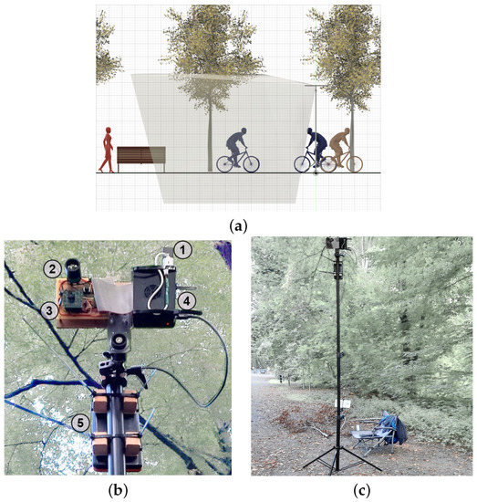
Figure 1.
(a) Schematic mounting concept of sensor showing alignment and field of view, (b) close up of mounted sensor system consisting of (1) an NM500 evaluation USB stick, (2) an 80 × 64 sensor, (3) a 160 × 120 sensor, (4) a Raspberry Pi4, and (5) a battery pack. (c) Full view of mounted sensor system.
We evaluated the concept in multiple series of indoor and outdoor tests. The tests showed that by using the low-resolution thermal images, the system was capable of monitoring different scenes independent of the lighting conditions, fulfilling requirements 1 and 2. In our test, the prototype was mounted on the side of the road using a tripod for mobile lighting installations and mounting clamps for consumer cameras as seen in Figure 1b,c. The prototype was powered by a consumer-grade powerbank. Even with the sensors and optics detached for transport, the system could be set up by a single person within 10–15 min.
Based on a series of field tests, we concluded that positioning the LWIR camera at a height of 3 m and angled toward the ground yielded the most accurate results (see Figure 1 for details). With this position, objects in the front do not fully obstruct objects in the back. Thus, people walking or driving side by side can be distinguished easier. At the same time, a partial profile view leads to better classification results than a full frontal view.
Based on our observations during our field tests, we extended our concept with an additional low-power radar sensor. Figure 2 shows a rendering of the extended prototype with an additional radar module. The prototype was designed as an extension board compatible with the Raspberry Pi platform. It comprises integrated voltage regulators that allow the use of a 12 V lead acid battery as a power supply. The purpose of the additional radar is to work as a trigger for the other sensors. This allows one to power down most components during periods of no activity to extend the battery life.
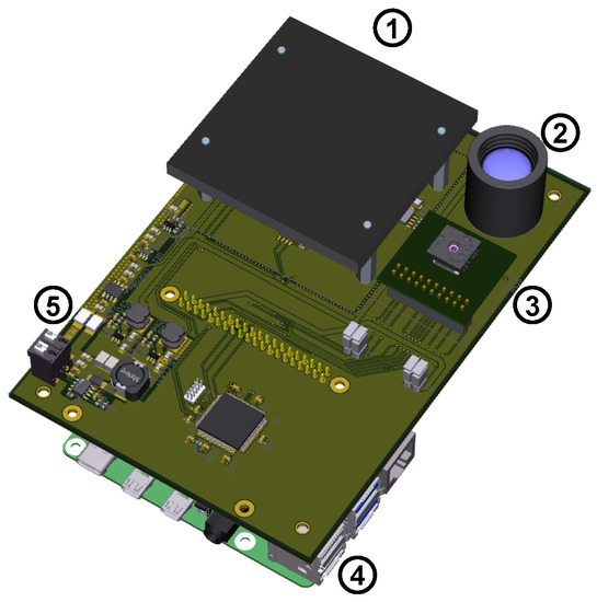
Figure 2.
Rendering of the extended prototype, showing (1) radar, (2) 80 × 64 pixel LWIR sensor, (3) 160 × 120 pixel LWIR sensor, (4) Raspberry Pi 4, and (5) power supply and Radar-MCU.
3.2. Sensors
As stated by Planck’s law, all objects emit radiation in a wide range of wavelengths [9]. The maximum of this radiation depends on the body’s temperature, as visualized in Figure 3. For bodies colder than 3000 K, most of the emitted radiation lies in the infrared spectrum. Therefore, to measure the temperature of most bodies, it is necessary to use sensors sensible for wavelengths above 1 µm.
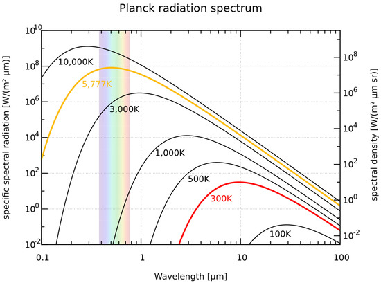
Figure 3.
Black–body spectrum for different temperatures. Temperature of the Sun is marked in yellow, and typical ambient temperature is marked in red [10].
DIN 5031 and the International Commission on Illumination define areas IR-A, IR-B, and IR-C, while ISO 20473 gives the designations and classifications in the near-infrared (NIR), middle-infrared (MIR) and far-infrared (FIR) ranges. The term LWIR is not officially defined by a norm but is commonly used and encompasses the area of 8–15 µm, therefore lying in the range of MIR and IR-C. Translated to emitting temperatures, long-wave infrared (LWIR) radiation is emitted by objects of a temperature between 193 K and 362 K. For this reason, LWIR sensors are well suited to monitoring everyday objects.
The two most common types of sensors for detecting LWIR radiation are photon detectors and bolometers. Photon detectors consist of semiconductor chips which detect incoming light, similiar to digital cameras, by utilizing the inner photoelectric effect [11]. It is necessary to cool these detectors to low temperatures because the necessary bandgaps only become available at low temperatures. This additional cooling is the reason why most of these cameras are quite large and require a high amount of power. The other kind of sensor is bolometers. Bolometers work through the absorption of incoming light and detecting the resulting rise in temperature. Modern advances in micro-manufacturing techniques allow for the construction of arrays of bolometers with a pixel pitch below 12 µm. Such bolometers are often referred to as microbolometers, offering the advantages of a lower size and lower cost and power consumption, but they typically have more noise and lower sensetivity when compared with photon detectors.
Due to power and cost constraints, we decided to use bolometer sensors for our project. In preceding projects, we compared different bolometer sensors with different resolutions, technologies, and fields of view (FoVs). For our proof-of-concept system, we settled on a sensor with a resolution of 160 × 120 pixels and a FoV of 57°. In our previous work, we showed that sensors with lower resolutions are also suitable [2]. The decision was based on a lower noise-equivalent temperature difference (NETD) and a more suitable FoV of the 160 × 120 pixel sensor.
3.3. The Neuromorphic Processor
The neuromorphic processor used for our application was the NM500, developed by Nepes and General Vision. The decision to use this chip was made based on the three main features of this chip: low power consumption (7 mW), fixed latency (classification in 19 clock cycles, only requiring 9.1 µs for classification and readout), and self-learning (the chip can perform learning operations on its own within the time it takes to perform a classification).
The chip’s architecture was based on the NeuromMem technology developed by General Vision [12]. In contrast to multipurpose processors, the NM500 utilizes 576 identical components called neurons, forming a neural network which can approximately be described as a three-layer radial basis function (RBF) network. Additionally, the chip can switch between RBF and k-nearest-neighbors (KNN) classification. Each neuron contains memory for storing a feature vector called a model, an arithmetic unit, and registers for configurations. This configuration allows each neuron to perform operations independent of each other. Multiple chips can be used in parallel to increase the capacity of the network. For added flexibility, the neurons can be configured as subnetworks, called context, either within one single chip or within a cluster of multiple chips. This allows performing multiple classification tasks without the need of loading a new network from memory or retraining the chip. This is helpful if multiple sensors are used for classification or to accommodate certain conditions, such as night and day.
When performing a classification, a feature vector is transmitted to the network together with a context identifier. After receiving the feature vector, each neuron in the requested context will calculate the distance between the input vector and the stored model. The arithmetic unit of each neuron is capable of calculating the distance using Supremus- or L1-Norm:
Based on the chip’s setting and the distance, the neuron decides if it enters the firing stage. In KNN mode, every neuron will fire, while in RBF mode, only neurons with a distance inside the active influence field will fire. The active influence field is set during training. All neurons in the firing stage will then compete for the lowest distance, and the chip will signal when it is ready. When querying the results, the chip will always return the neuron in the firing stage, starting with the lowest distance. This way, it is not necessary to read numerous neurons after each classification.
A powerful feature of this architecture is the capability of performing supervised learning with no external processing required. To perform learning, the process is similar to the process of classification described above. In addition to a feature vector and context identifier, a class ID is transmitted to the chip. The network will then perform a regular classification. Depending on the classification results, the chip will either commit a new neuron or adapt the active influence fields of the neurons already committed. If no neuron is in the firing stage, a new neuron will be committed, and the active influence field will be set to the default value of the maximum influence field. A new neuron will also be committed if only neurons with wrong class IDs are in the firing stage. The active influence field of the new neuron will be set to the distance value of the first neuron in the firing stage. Then, the active influence field of each neuron in the firing stage will be reduced below the active influence field of the new neuron. If neurons of the right and the wrong class IDs are present in the firing stage, then no new neuron will be committed. The active influence field of neurons with the wrong class IDs will be reduced below the distance value of the closest neuron with the correct class ID. If no uncommitted neurons are available, hten only the reduction of the influence fields will be performed. If the active influence field of a neuron is set below the threshold of the minimal influence field, then the neuron will be flagged as degenerated. It will still take part in classification and learning, but the active influence field will not be reduced any further. Degeneration of a neuron either designates a bad sample or that a clear distinction between two classes is not possible, with the latter being the case for multiple neurons degenerating. The values of the maximum and minimum influence fields can be set individually for each context.
3.4. Software Concept
Before being provided to the NM500 neuromorphic processor, the raw data need to be preprocessed. Figure 4 visualizes the flow of data from the source, sensor, or memory to the NM500, as designed in our previous work. On the right side, the intermediary steps of one exemplary image processing flow are shown. The task of the image processing flow is data reduction from a 160 × 120 array (38.4 kB) to a feature vector of 256 bytes for classification. To avoid extensive on-site sensor calibration, our algorithms only use relative temperature differences for classification rather than the absolute temperatures.
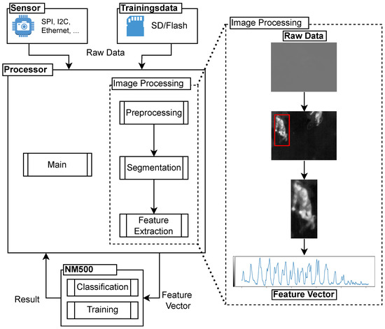
Figure 4.
Conceptual data flow.
Figure 5 shows the next evolution stage of our preprocessing chain. One of our goals was to implement a modular design to easily change parts of the implementation to evaluate different algorithms. The main difference in the new data flow is that preprocessing is no longer an independent component, and segmentation was split into background subtraction and detection. In addition, feature extraction now has two inputs: (1) the original image and (2) an object list. The object list contains information about the objects present in the image (e.g., the object’s contour). These changes were made because background substraction and feature extraction were implemented independent of one another and required different image preprocessing steps.
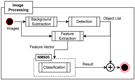
Figure 5.
Data processing implemented with NM500.
4. Evaluation
4.1. Set-Up
For the evaluation of our concept, we designed a simple prototype based on a Raspberry Pi 4 (RPI4) to interface with development kits for the sensors and the NM500. This allows for easy implementation of data logging and processing while still being mobile and compact. The LWIR sensor used had a resolution of 160 × 120 pixels for a field of view (FOV) of 57° and a frame rate of 9 frames per second. Our protorype set-up is shown in Figure 1b,c. We performed a series of indoor and outdoor tests. The outdoor tests were performed in different locations in a public park. In the park, we tested the performance with different surfaces, including gravel, asphalt, and grass. Due to privacy concerns, the performance in these outdoor settings was only judged using the live image, and no data including persons were stored and processed further. To acquire data without privacy concerns for further testing, we performed an indoor test with a small group of participants. During the indoor test, we took images of bikes, e-bikes, scooters, e-scooters, and cargo bikes. The sensors were mounted at a height of 3.5 m and an inclination of 20° and rotated 45° toward the road.
During the indoor test, we acquired more than 40,000 images. This set of images was then filtered. First, all images without objects of interest were excluded, and then the labeling was performed. During labeling, the classes of bike (Bike), pedestrian (Pede), scooter (Scoo), and cargo bike (Carg) were distinguished. In addition, objects overlapping each other were given an additional label. After labeling, the images were downsampled to simulate a frame rate of two frames per second to match our concept and reduce similarities inside the dataset. Lastly, it was decided to exclude overlapping objects from the scope of this work and evaluate these cases in a future work. After filtering, 4400 objects of interest remained in the dataset. All further development of the algorithms was performed using this dataset.
4.2. Evaluation Method
The previous work already proved that our concept is capable of performing multi-class classification tasks. The focus of this work is the comparison of different feature extraction methods. For each change in the feature extraction algorithm, a seperate test was performed as visualized in Figure 6. First, the dataset was shuffled and split into 70% training data and 30% validation data. If required by the feature extraction method, a mapping function was calculated based on the training data. The mapping function was not calculated using the whole dataset to ensure that no information from the validation data was present in the training process. After that, the feature vector was calculated, and the training was performed. Following the reference guides [13], the training data were then ordered such that repetition in the class ID would only appear after each additional class ID was trained. This structuring ensures that the chip always learns enough counterexamples to set the influence field for existing neurons. Training was repeated until no more new neurons were committed and no changes in the influence fields occurred. This usually took four to five epochs.
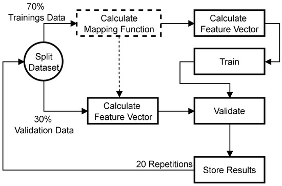
Figure 6.
Steps performed for training and evaluation.
Preliminary tests showed that the random selection of images could influence the results. To obtain an average performance, all tests were repeated 20 times with randomly picked data before being evaluated.
4.3. Metrics
To measure the performance of the classification, we used a system of four binary classifiers and sorted the results as shown in Figure 7. Based on this sorting, we calculated the performance metrics. We used the F1 score to measure the performance per class:
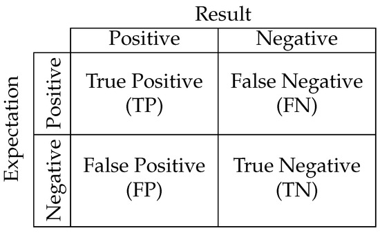
Figure 7.
Possible results for binary classifiers.
We used the weighted average score to compare different test series:
Here, N is the number of classes, is the F1 score for class C, and is the number of correct results in class c. If not otherwise stated, the F1 score along the standard deviation (sigma) of the test series is given in all following tables and plots.
4.4. Feature Extraction
We focus on four ways to extract feature sets, namely the scaled region of interest (ROI), ROI histogram, contour features, and moments. For each, we also test different implementations and combinations of preprocessing algorithms and the combination of different feature sets for classification.
Scaled ROI: We created the first feature set the same way as in the preliminary proof of concept by first extracting the ROI and then scaling the image segment down to less than 256 pixels before flattening the segment row by row. As a way of preprocessing the data, we focused on normalization, as our preliminary tests showed that other contrast enhancement methods, such as histogram equalization and contrast-limited adaptive histogram equalization (CLAHE), yielded worse results. First, we examined the difference between global and local normalization of the ROI while keeping the final segment size of 16 × 16 pixels. The result was a slightly better performance of the local normalization, as shown in Table 3. The second series of tests focused on the size and aspect ratio of the extracted image segment. We performed three tests with sizes of 10 × 20, 13 × 19, and 12 × 19 pixels. Then, the sizes of 13 × 19 and 12 × 19 pixels were chosen because they were close to the median aspect ratio of all objects in the dataset, while 10 × 20 pixels was chosen as an example in which neither aspect ratio was ideal, nor was the whole feature vector used. The results show that all feature sets performed similar and that local normalization was slightly better than global normalization.
Table 3.
F1 score results of the test series with normalized image segments (scaled ROI) for k-nearest neighbors (KNN) and radial basis function (RBF) modes.
ROI histogram: The second series of feature sets was created using the histogram of the pixel values in the ROI. The histogram was defined to have 256 bins, and the sizes of the bins were defined dynamically for each image. We examined the performance of two approaches for how to handle bins that contain more than 255 elements. The first one was normalizing all histograms between 0 and 255, and the second approach was limiting the size of a bin to 255. The results in Table 4 show that limiting the bins achieved better classification results.
Table 4.
F1 score results of the test series with histograms.
Contour features: The next set of features was not extracted from the image region itself but from the geometric attributes of the object’s contour. The specific features used were the height, width, circumference, aspect ratio, area, extent, solidity, and orientation. The extent was calculated as the quotient of the contour area and bounding box area. Solidity is the ratio between the contour area and the area of a convex hull around the contour [14].
To use these features for classification, it is necessary to perform a transformation to fit the data into one byte of resolution available per feature. Each feature requires a specific transfer function, as the range of possible values differs greatly. An additional consideration is that not all possible values were actually present in the dataset. For example, the aspect ratio could be any value between 0 and 160 in theory, but the dataset contained no objects with an aspect ratio larger than 5, and most aspect ratios were below 1. This fact could be used to increase the available resolution for the significant range of values.
We investigated the performance of three different transfer functions in combination with the geometric contour features (Table 5). For each transfer function, we first identified the actual range of values in the training dataset and defined an expected value range. Values outside this expected range would be mapped to 0 for values lower than expected and 255 for higher values. Figure 8 shows these transfer functions and the histogram of the original and resulting values for the example of the aspect ratio. The first transfer function is a linear transformation, normalizing the expected values into the range between 0 and 255. Figure 8b shows that the shape and distribution of the histogram remained unchanged. The second transfer function we investigated was the histogram equalization. Figure 8c shows that the resulting histogram then spread over the entire value range, which should have resulted in a more efficient use of the available feature size. However, histogram equalization is computation-intensive. As a compromise between efficient linearization and histogram equalization, we investigated a third transfer function: partial linearization. For this, we first identified the 10th and 90th percentiles and defined a normalization for the equivalent value range in the feature vector. The results of partial linearization are presented in Figure 8d.
Table 5.
F1 score results of the test series with contour properties.
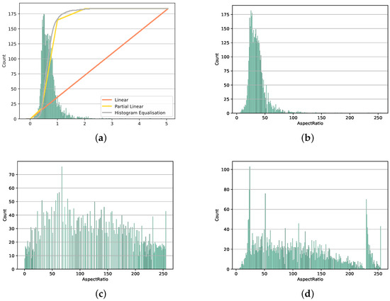
Figure 8.
Visualization of the transfer function and the value range before and after mapping at the example for the aspect ratio. (a) Original value range and transfer functions (b) with linear mapping, (c) with histogram equalization, and (d) with partial linear mapping.
Moments: The last method of feature extraction we investigated was the use of image moments. In addition to the common moments defined by Equation (5), multiple subsets of moments can be derived with different properties [15]. We investigated three additional sets of moments: (1) the translation-invariant central moments calculated using Equation (7), (2) the scaling-invariant normalized moments (see Equation (8)), and (3) the rotation-invariant Hu moments (see Equations (9)–(15)):
In the following, we used moments up to the third order and omitted moments that were either duplicates or constants, as these contained no additional information. The whole feature vector consisted of 31 features, 10 basic moments, 7 central moments, 7 normalized moments, and 7 Hu moments.
Similar to the contour properties, the moments had to be mapped to values between 0 and 255. For this, we used the same functions as before. The results are shown in the first two major columns of Table 6, indicating a performance of less than 40. The value ranges and mapping functions were identified as the root cause for the poor performance:
Table 6.
F1 score results of the test series with image moments.
Mapping the moments to a logarithmic scale and keeping the sign (see Equation (16)) yielded improvements. As shown in the last three major columns of Table 6, we could nearly double the performance.
In addition to using the image moments, we investigated the contour moments calculated using Green’s theorem and the line integral of the object’s contour. Again, we used the same mapping functions as before, including the logarithm. The results are shown in the first three columns of Table 7. The last two columns contain the results for a series of tests that did not include all previously mentioned moments but only basic moments and central moments.
Table 7.
F1 score results of the test series with log contour moments.
Combined feature sets: As a last set of features, we investigated the combination of different feature extraction methods. First, we combined the contour properties and a reduced set of 16 contour moments and used histogram equalization as a mapping function. The moment was omitted, as it was equal to the contour surface and already part of the contour properties. The results are shown in Table 8, where in column (a), the performance was slightly better than the results of the reduced moments.
Table 8.
F1 score results of the test series with combined feature extraction methods. (a) Combination of contour properties and contour moments. (b) Image moments of a downscaled ROI. (c,d) Combination of scaled ROI and contour moments. (c) The 12 × 19 pixel resolution and 24 moments. (d) The 12 × 18 pixel resolution and 31 moments.
The second combination we tried reduced the computational load by first downscaling the ROI to 16 × 16 pixels and then calculating the image moments. The results are shown in Table 8, where column (a) shows that the performance was 7–9 percent worse than the performance of the unscaled image moments.
The last combination tested was a combination of the scaled ROI and the image moments. We already showed that by changing the aspect ratio of the final feature segment, the classification results were nearly unaffected, and the necessary amount of features could be reduced. We used an ROI 12 × 19 pixels in size in combination with the reduced set of 24 moments. The results are shown in the last two columns of Table 8, where for column (c), an ROI of 12 × 19 pixels and a reduced set of 24 moments were used, and for column (d), an ROI of 12 × 18 pixels and the full set of moments were used.
4.5. Training Behavior
In another series of tests, we focused on the training behavior of the NM500. Our goal was to estimate the number of neurons required to perform classification. This number would then yield the number of NM500 ICs required. The results are shown in Figure 9. The number of committed neurons increased nearly linearly with the number of training images. The accuracy, however, did not follow the same trend. The accuracy for both the KNN and RBF modes approached a fixed value. Additionally, the number of neurons committed to a class was not connected to the accuracy. The pedestrian and bike classes had similar numbers of committed neurons but achieved very different classification accuracies.
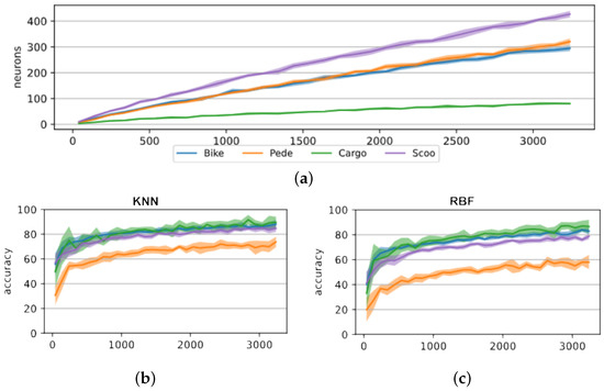
Figure 9.
Training behavior of the NM500 with increased number of images in the training dataset, with feature extraction using scaled region of interest of 16 × 16 pixels. (a) Neurons committed per class. (b) Classification accuracy in KNN mode. (c) Classification accuracy in RBF mode.
5. Results
Table 9 summarizes the best results of each approach, and Figure 10 shows the results for each class of these feature sets. Each of these plots show a similar outline, with pedestrian as the worst recognized class and cargo bike as the best one, except for the contour features, where cargo bike was the second-worst class. The general distribution of the results can partially be explained by the size of the vehicle compared with the size of the driver and the variety of vehicles. We only had a single cargo bike, and it was the largest vehicle in our test set-up. Changing the driver did not influence the overall appearance or silhouette of the object as much as in other classes. This is further supported by Figure 11, which shows that the cargo bike class was the only class with no significant amount of unknown classifications. The bike, as the second-largest vehicle, had the second-highest score on average. Even if the contrast did not always allows seeing the bike in the thermal image, the vehicle forced the driver into a certain position, which could be distinguished. The same applied to the scooter; all scooters forced the driver into a certain position. Pedestrians that were not constrained by a vehicle had the largest variety in posture and were therefore the hardest to distinguish.
Table 9.
Best F1 score results of the tested feature extraction methods.
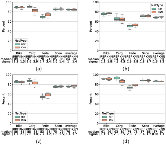
Figure 10.
Best results for the tested feature extraction methods: (a) scaled ROI, (b) contour features, (c) contour moments, and (d) combined moments and scaled ROI.
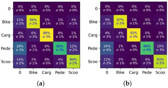
Figure 11.
Row-wise normalized RBF confusion matrices of (a) 16 × 16 scaled ROI and (b) 12 × 18 combined scaled ROI and contour moments, with true labels on the y axis and predicted labels on the x axis.
In addition, further inspection of the results shows that the errors in the classification of the cargo bike could also be attributed to partially inadequate labeling (see Figure 12). The manual process allowed for labeling images in the context of the previous and following images, which in turn allowed for the labeling of small object segments. These rare and adverse occurrences led to errors in classification.
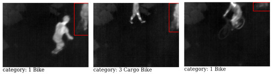
Figure 12.
Examples for adverse labeling, the red box marks the ROI of the labeld object.
Figure 11 shows the confusion matrices of the results for the RBF mode of the initial tests with a scaled ROI and the final test with a scaled ROI combined with the contour moments. On the left axis, the expected label is shown, and on the bottom axis, the predicted label is shown. The “0” row and column show the results if no decision could be made. The first row is empty because the datasets did not contain any examples for no classes. The confusion matrices show that the change in the aspect ratio and the addition of moments had no adverse effects, the classification accuracy for each class went up, and a wrong detection did not shift classes.
6. Conclusions
In this paper, we demonstrated the significant improvement of our previous concept for a low-power multi-class micromobility vehicle counting system utilizing neuromorphic processing and low-resolution thermal imaging arrays. In field tests, we verified that the sensors are capable of performing under real-world conditions and that our concept for the set-up is feasible. We improved on both our hardware and software design with our prototype. By combining the features extracted from the image and the object’s contour, we improved our classification accuracy (F1 score) to over 90% (compare with Figure 10) for certain classes and to an average of 87% (compare with Table 9). We used fully automated data segmentation algorithms, and we are confident that these approaches can be developed further to obtain a classification accuracy close to those of the hand-segmented approaches. With outdoor tests, we could demonstrate that the implemented concept is feasible.
For future work, we suggest the following aspects to be considered:
- Training data:Most important for the next step in development is to conduct further testing in an outdoor environment, acquiring more data.
- Self-learning:The current approach does not yet fully utilize the NM500’s capability for self-learning. It could be used to allow the system to learn during operation and thus independently adapt to new environments.
- Multi-step classification:In this work, we optimized the performance by combining features from different sources into one feature vector. It could also be feasible to perform multiple classifications using different feature sets and interpret the different results in combination.
- Utilization of the NM500:The current task of the NM500 is just the final classification, as preprocessing, segmentation, and detection are still performed on the host system. It should be evaluated which tasks could also be performed by the NM500.
- Sensor fusion:The new generation of our prototype utilizes a low-power radar as a trigger for the infrared sensors. It should be investigated how the information of both sensors could be used in a sensor fusion approach to further enhance the performance.
In addition, the current concept of using radar information as a trigger and only reduced thermal still images may give away a lot of information potential. While evaluation of the complete LWIR full motion data flow does not comply with the power consumption requirements, using a sequence of at least multiple (3–5) frames could further improve the overall performance. For application scenarios allowing wall plug power, additional processing concepts might be considered, making use of the full motion data of the LWIR camera. Finally, different sensor sets could then be considered, including 3D time-of-flight cameras [16,17]. Such systems have also shown promising results in a parallel development path of this project. These results will be presented in a separate publication.
Author Contributions
Writing—original draft preparation, B.S.; review and editing, R.L.; supervision, J.A. and R.L. All authors have read and agreed to the published version of the manuscript.
Funding
This project was supported by the Federal Ministry for Economic Affairs and Energy (BMWi) on the basis of a decision by the German Bundestag. Funding code: ZF4190305GR9.
Institutional Review Board Statement
Not applicable.
Informed Consent Statement
Informed consent was obtained from all subjects involved in the study.
Data Availability Statement
Not applicable.
Conflicts of Interest
The authors declare no conflict of interest.
References
- CPSC. Micromobility Products-Related Deaths, Injuries, and Hazard Patterns: 2017–2020. Available online: https://www.cpsc.gov/s3fs-public/Micromobility-Products-Related-Deaths-Injuries-and-Hazard-Patterns-2017-2020.pdf?VersionId=s8MfDNAVvHasSbqotb7UC.OCWYDcqena (accessed on 17 February 2023).
- Stahl, B.; Lange, R.; Apfelbeck, J. Evaluation of a concept for classification of micromobility vehicles based on thermal-infrared imaging and neuromorphic processing. In Proceedings of the SPIE Future Sensing Technologies 2021, Online, 15–19 November 2021; Kimata, M., Shaw, J.A., Valenta, C.R., Eds.; SPIE: Bellingham, WA, USA, 2021; p. 6. [Google Scholar] [CrossRef]
- Ozan, E.; Searcy, S.; Geiger, B.C.; Vaughan, C.; Carnes, C.; Baird, C.; Hipp, A. State-of-the-Art Approaches to Bicycle and Pedestrian Counters: RP2020-39 Final Report; National Academy of Sciences: Washington, DC, USA, 2021. [Google Scholar]
- Nordback, K.; Marshall, W.E.; Janson, B.N.; Stolz, E. Estimating Annual Average Daily Bicyclists: Error and Accuracy. Proc. Transp. Res. Rec. 2013, 2339, 90–97. [Google Scholar] [CrossRef]
- Klein, L.A. Traffic Flow Sensors; Society of Photo-Optical Instrumentation Engineers: Bellingham, WA, USA, 2020. [Google Scholar]
- Larson, T.; Wyman, A.; Hurwitz, D.S.; Dorado, M.; Quayle, S.; Shetler, S. Evaluation of dynamic passive pedestrian detection. Transp. Res. Interdiscip. Perspect. 2020, 8, 100268. [Google Scholar] [CrossRef]
- Gajda, J.; Sroka, R.; Stencel, M.; Wajda, A.; Zeglen, T. A vehicle classification based on inductive loop detectors. In Proceedings of the 18th IEEE Instrumentation and Measurement Technology Conference. Rediscovering Measurement in the Age of Informatics (Cat. No.01CH 37188), Budapest, Hungary, 21–23 May 2001; pp. 460–464. [Google Scholar] [CrossRef]
- Yang, H.; Ozbay, K.; Bartin, B. Investigating the performance of automatic counting sensors for pedestrian traffic data collection. In Proceedings of the 12th World Conference on Transport Research, Lisbon, Portugal, 11–15 July 2010; Volume 1115, pp. 1–11. [Google Scholar]
- Planck, M. Faksimile aus den Verhandlungen der Deutschen Physikalischen Gesellschaft 2 (1900) S. 237: Zur Theorie des Gesetzes der Energieverteilung im Normalspectrum. Phys. J. 1948, 4, 146–151. [Google Scholar] [CrossRef]
- Prog. File:BlackbodySpectrum Loglog de.svg. Available online: https://commons.wikimedia.org/wiki/File:BlackbodySpectrum_loglog_de.svg (accessed on 22 January 2022).
- Einstein, A. Über einen die Erzeugung und Verwandlung des Lichtes betreffenden heuristischen Gesichtspunkt. Ann. Phys. 1905, 322, 132–148. [Google Scholar] [CrossRef]
- General Vision Inc. NeuroMem Technology Reference Guide, 5.4 ed.; General Vision Inc.: Petaluma, CA, USA, 2019; Available online: https://www.general-vision.com/documentation/TM_NeuroMem_Technology_Reference_Guide.pdf (accessed on 15 March 2023).
- General Vision Inc. NeuroMem RBF Decision Space Mapping, 4.3 ed.; General Vision Inc.: Petaluma, CA, USA, 2019; Available online: http://www.general-vision.com/documentation/TM_NeuroMem_Decision_Space_Mapping.pdf (accessed on 15 March 2023).
- OpenCV: Contour Properties. Available online: https://docs.opencv.org/3.4/d1/d32/tutorial_py_contour_properties.html (accessed on 7 March 2023).
- Hu, M.K. Visual pattern recognition by moment invariants. IEEE Trans. Inf. Theory 1962, 8, 179–187. [Google Scholar] [CrossRef]
- Lange, R.; Seitz, P. Solid-state time-of-flight range camera. IEEE J. Quantum Electron. 2001, 37, 390–397. [Google Scholar] [CrossRef]
- Lange, R.; Böhmer, S.; Buxbaum, B. 11—CMOS-based optical time-of-flight 3D imaging and ranging. In High Performance Silicon Imaging, 2nd ed.; Durini, D., Ed.; Woodhead Publishing Series in Electronic and Optical Materials; Woodhead Publishing: Cambridge, UK, 2020; pp. 319–375. [Google Scholar] [CrossRef]


Disclaimer/Publisher’s Note: The statements, opinions and data contained in all publications are solely those of the individual author(s) and contributor(s) and not of MDPI and/or the editor(s). MDPI and/or the editor(s) disclaim responsibility for any injury to people or property resulting from any ideas, methods, instructions or products referred to in the content. |
© 2023 by the authors. Licensee MDPI, Basel, Switzerland. This article is an open access article distributed under the terms and conditions of the Creative Commons Attribution (CC BY) license (https://creativecommons.org/licenses/by/4.0/).