Article

A Methodology for Continuous Monitoring of Rail Corrugation on Subway Lines Based on Axlebox Acceleration Measurements

Department of Mechanical Engineering, Politecnico di Milano, Via G. La Masa, 1, 20156 Milan, Italy
*
Author to whom correspondence should be addressed.
Appl. Sci. 2023, 13(6), 3773; https://doi.org/10.3390/app13063773
Submission received: 29 January 2023 / Revised: 10 March 2023 / Accepted: 14 March 2023 / Published: 15 March 2023
(This article belongs to the Special Issue Alternative Techniques in Vibration Measurement and Analysis)

Abstract

:
Rail corrugation is a degradation phenomenon that manifests as a quasi-periodic irregularity on the running surface of the rail. It is a critical problem for urban railway lines because it induces ground-borne vibrations transmitted to the buildings near the infrastructure, causing complaints from the inhabitants. A typical treatment to mitigate the rail corrugation problem is the periodic grinding of the rails, performed by dedicated vehicles. The scheduling of rail maintenance is particularly critical because it can be performed only when the service is interrupted. A procedure for the continuous monitoring of rail corrugation is proposed, based on axlebox acceleration measurements. The rail irregularity is estimated from the measured acceleration by means of a frequency domain model of vertical dynamics of the wheel–rail interaction. The results obtained by using two different methods (a state-of-the-art method and a new one) are compared. Finally, the study of the evolution of the power content of the rail irregularity enables the identification of the track sections where corrugation is developing and rail grinding is necessary.

1. Introduction

In recent years, the effort in finding “environmentally friendly” solutions for the transport of passengers and freight is significantly increased. Urban railway transport is an attractive solution to this aim thanks to its high capacity compared to road traffic. This helps to reduce traffic congestion and air pollution in metropolitan areas. Despite these benefits, the high static loads combined with the high dynamic forces caused by the rail unevenness induce vibrations that may be the cause of several issues.
Among others, rail corrugation is one of the major problems related to urban railway lines. It consists of the appearance of a quasi-periodic irregularity on the running surface of the rail that causes ground-borne vibrations, along with secondary noise radiation, and, if it is well developed, degradation of vehicle and track components. The nucleation of rail corrugation is not imputable to a single phenomenon, but different types exist that differ in the characteristics and in the root causes [1,2,3]. It is worth mentioning that even if the root causes are different, in any case they are associated with the dynamics of the wheel–rail interaction. In [4], lately reviewed in [5], a classification of the different types of rail corrugation has been proposed.
Rail corrugation affects most of the railway lines [4,5], but it is a critical problem for urban lines, e.g., subways, because the induced vibrations propagate from the track infrastructure to the neighbouring buildings through the soil, causing complaints by the inhabitants. At low frequencies, the discomfort is due to the human sensitivity to whole-body vibration, while at higher frequencies, in the audible frequency range, it is perceived in terms of rumble noise.
Mitigation measures addressing the different types of rail corrugation are proposed in [3,6]. However, the most effective require modifications in vehicle or track architecture and therefore they are less suitable for existing systems. Moreover, a treatment may avoid the occurrence of a specific corrugation class but could favour the formation of a different corrugation type. The usage of different speed profiles, when possible, or friction modifiers typically reduces the corrugation growth rate, but, in general, does not prevent its formation.
The most used mitigation action against corrugation is the reprofiling of the rail running surface by means of grinding vehicles when the service is interrupted. This maintenance operation is particularly critical for railway infrastructure managers from both an economical point of view, due to the high initial and operative costs of grinding vehicles, and a managerial point of view, due to the limited time available for such operations. For these reasons, it would be convenient to perform rail grinding only when and where it is strictly necessary.
To this aim, the continuous monitoring of rail irregularity along the line will be helpful in locating track sections where corrugation is forming and evolving. Different techniques for the measurement of the longitudinal railhead profile are proposed in [7].
The most promising technique for the measure of the railhead profile at service speeds is the estimation of the irregularity by means of accelerometers mounted in correspondence to the axleboxes of a commercial vehicle. An attempt with a chord-based measurement system is proposed in [8], in which rail roughness is measured at service speed by means of optical sensors mounted on a train bogie. However, the performance of this system depends on the vehicle speed and weather conditions, and its reliability can be significantly affected by dust or other factors in harsh environments.
Tufano et al. [9] estimate rail roughness by using a hybrid multi-sensor approach in which acceleration signals are combined with acoustic measurements. A model-based estimation of acoustic rail roughness from axlebox acceleration measurements is proposed by Pieringer and Kropp in [10], in which a time domain approach is used. Even if the results are promising, the considered axlebox acceleration signals are not measured, but generated numerically by using the proposed model of the wheel–rail interaction. In the aforementioned work a refined model of the wheel–rail interaction is used, since the frequency range of interest for acoustic problems is in the order of some kHz. On the other hand, the maximum frequency concerning the rail corrugation phenomenon on subway lines ranges from 400–600 Hz, depending on the maximum speed reached by the vehicles. For this reason, simplified models can be considered.
An axlebox accelerometer measurement system used for the identification of track sections affected by rail corrugation is the HRSCA system presented in [11], in which the Root Mean Square (RMS) of rail irregularity is estimated by using a frequency domain model of the wheel–rail interaction. This technique is attractive because measurements can be taken at service speed and accelerometers are relatively cheap. They can be mounted on commercial vehicles with the purpose of monitoring the whole network, reducing the time required to perform the same operation with diagnostic trains.
The objective of this work is to propose a modification of the HRSCA system to be applied to axlebox acceleration data from a commercial vehicle running on a subway network. A more refined model of the wheel–rail interaction for the calculation of the transfer function of the axlebox accelerometer measurement system is introduced, in order to improve its effectiveness in monitoring rail corrugation. The dynamics of the wheel–rail interaction is studied by characterising the dynamic behaviour of the wheel and track as standalone systems. In particular, the wheel is modelled as a point mass in [11], while a flexible wheelset model resting on the primary suspension is used in the proposed approach. The transfer function of the measurement system is then calculated by coupling wheel and rail dynamics. The performances of the two methodologies are tested by analysing acceleration measurements from two runs of the diagnostic vehicle along a specific section of a subway network, where it is known that rail corrugation appears.

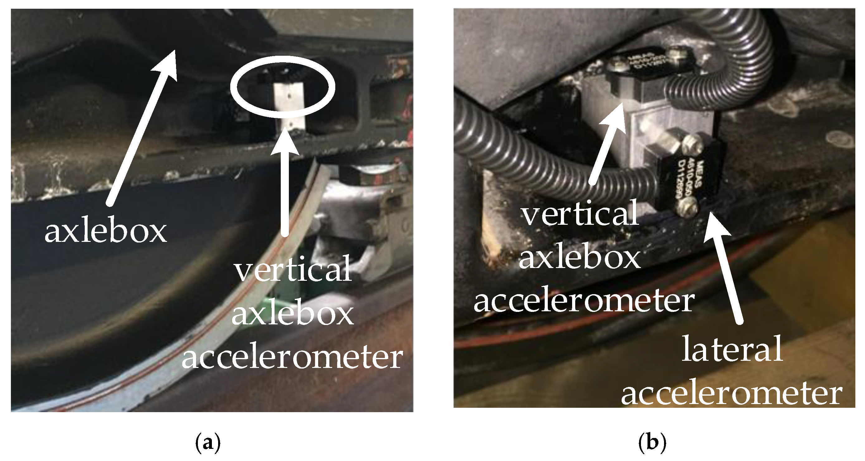
2. Description of the Measurement System

An axlebox accelerometer measurement system is installed on a trailer bogie of a commercial vehicle running on a subway network. It is made up of six accelerometers, an encoder and a gyroscope mounted on the carbody. Four accelerometers measuring the acceleration along the vertical direction are mounted on the axleboxes of the instrumented bogie, while two others measure the lateral acceleration of the wheelsets. As an example, the accelerometers mounted on the axleboxes of one of the instrumented wheelsets are shown in Figure 1. The absolute position of the vehicle along the line and the presence of curves are estimated by combining the speed signal from the encoder with gyroscope and lateral acceleration signals. The estimation of the position is facilitated by the stops of the vehicle in correspondence with the stations. The error in the estimation of the vehicle position is below a meter.
The estimation of rail corrugation from axlebox acceleration measurements, which is performed in the frequency domain, requires the determination of the transfer function of the measurement system [7]. It has the form:
H ( f ) = z i r r ( f ) z ¨ a x ( f ) ,
where f represents the frequency, z ¨ a x is the measured acceleration and z i r r is the rail irregularity. Being mounted on the axlebox, the measurement system is dynamically coupled with the vehicle. Thus, the transfer function must be determined by studying the dynamics of the wheel–rail interaction subjected to rail irregularity.

3. Transfer Function of the Measurement System
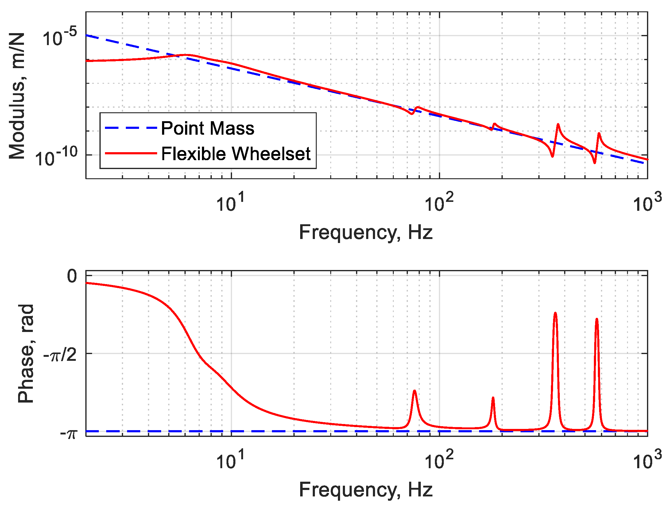
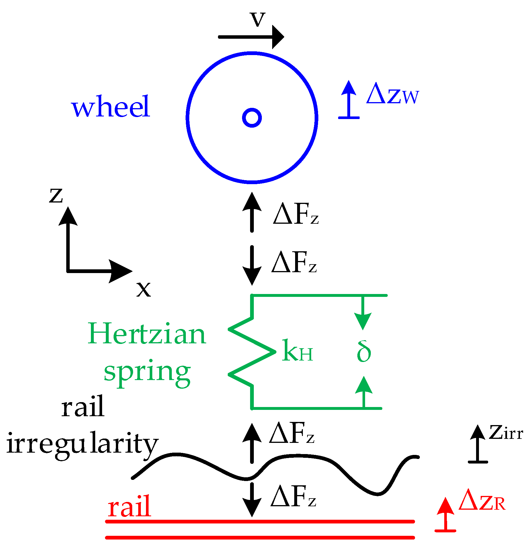
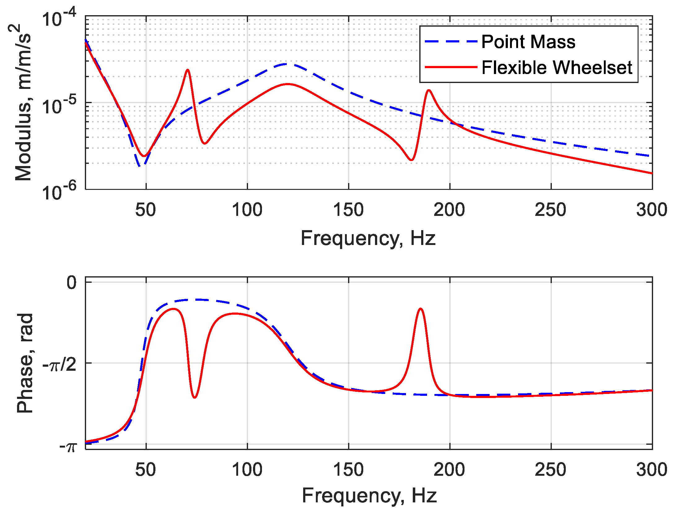
The calculation of the transfer function of the measurement system requires the prior knowledge of the dynamic behaviour of vehicle and track systems in the frequency domain. To this extent, the rail irregularity z i r r is assumed as a harmonic excitation at the wheel–rail interface that can be expressed as a function of the spatial coordinate x :
z i r r ( x ) = Z 0 e 2 π λ x ,
where Z 0 is the amplitude of the rail roughness and λ is the wavelength. The wheel running over the irregularity with a specified speed v defines an excitation frequency f according to the following relationship:
f = v λ ,
Since the spatial coordinate x can be expressed by the product of the speed and the time, the rail irregularity in time domain assumes the following form:
z ( t ) = Z 0 e Ω t Ω = 2 π f ,
where Ω is the circular frequency of excitation.
In high-frequency models for the wheel–rail interaction [12,13,14,15], the generic contact variable a ( t ) can be seen as the superposition of two different contributions:
a ( t ) = a 0 + Δ a ( t ) ,
The a 0 term is the steady-state component of the variable, while the second term Δ a ( t ) represents its dynamic fluctuation, varying harmonically as the irregularity. It is assumed in this work that rail irregularity generates fluctuations only in the vertical component of wheel–rail contact force and consequently in the vertical axlebox acceleration.
As a first step, the dynamic behaviour of the train and the track as standalone systems is obtained in terms of vertical direct receptance, i.e., the vertical displacement of the contact point on the wheel and the rail per unit vertical contact force. Concerning the vehicle dynamics, only the wheelset resting on the primary suspension is considered [16], because carbodies and bogies can be assumed dynamically decoupled from the wheelset given that the primary suspensions isolate bogie vibration in the frequency range of interest for rail corrugation (from 30 up to 300 Hz).

3.1. Wheel Dynamics

The main difference between the proposed model and the HRSCA system presented in [11] is in the model used for the description of wheelset dynamics. In [11], the wheel is modelled as a point mass M w running on the rail. The direct vertical receptance of the wheel, in this case, can be written as the following:
A W z ( f ) = 1 ( 2 π f ) 2 M w ,
However, the vibration modes of the wheelset are involved in almost all the different mechanisms that define the wavelength of rail corrugation [4,5], and therefore it is important to include them in the calculation of the wheel direct receptance.
To this aim, the dynamics of the wheel is derived by means of a modal model of the wheelset on the primary suspension. The mode shapes and the natural frequencies are obtained through a Finite Element Analysis (FEA) under the following assumptions:
  • The axle is modelled using 2D Euler–Bernoulli beam elements;
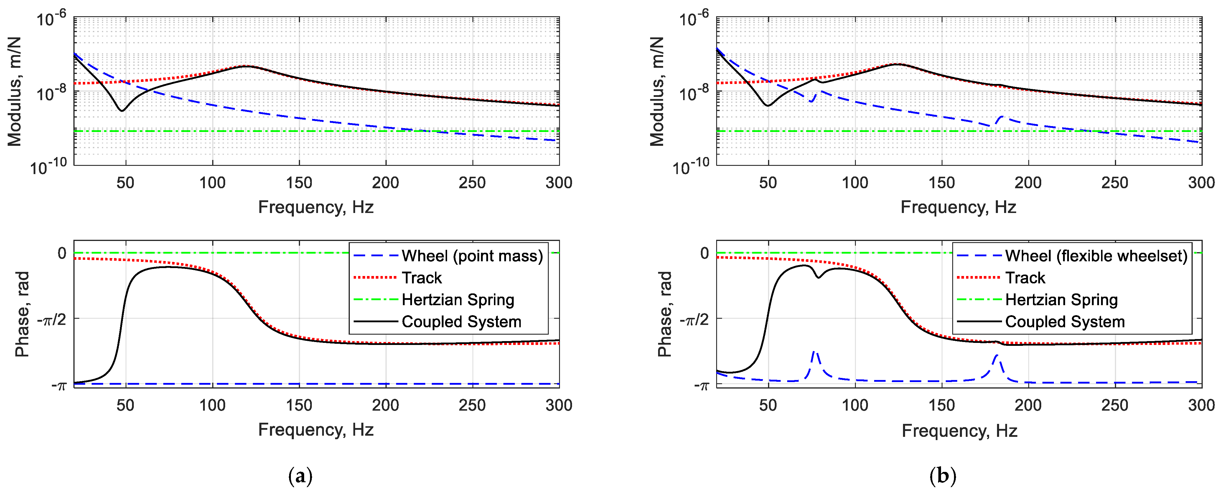
  • The wheels are considered as rigid bodies; due to the frequency range of interest for corrugation problems, the flexibility of the wheels does not have a strong influence on the different formation mechanisms [5];
  • The wheels and the brake disks are modelled as concentrated masses in their centre, accounting also for their moment of inertia;
  • The axleboxes are represented by concentrate masses placed in correspondence to their centre of gravity, while their rotational inertia is neglected;
  • The wheelset gyroscopic effect is neglected. The gyroscopic effect becomes significant at high speed [16,17,18]. On the considered subway line, speeds above 90 km/h are never reached. For higher speeds, the gyroscopic effect of the wheelset must be included in the analysis.
The data relative to the wheelset are summarised in Table 1.
The equation of motion of the wheelset has the following form:
[ M ] u ¨ _ + [ C ] u ˙ _ + [ K ] u _ = F _ ,
where F _ is the vector of the contact forces at the wheel–rail interface and u _ is the nodal displacements of the finite element model. The equation of motion is solved in modal coordinates by limiting to 800 Hz the mode shapes extracted from the FE model. This assumption is reasonable, since the frequency range of interest for the rail corrugation problem is limited to 300 Hz (in the present application). Due to the lack of experimental data on the structural damping of the wheelset, a modal damping ratio of 1% is assumed on all the bending modes. Damping ratios in this order of magnitude have been identified in an experimental modal analysis on a wheelset with similar characteristics.
The contact point is not included in the nodes of the finite element model, but thanks to the rigid wheel assumption, its displacement, and thus the receptance, can be derived. The procedure for the computation of the contact point receptance is outlined hereafter:
  • A unit vertical contact force is considered varying harmonically and it is applied to the wheel centre, also accounting for the transport moments;
  • The displacement vector of the wheel centre is defined by
X _ W c = { x W c y W c z W c φ x W c φ y W c φ z W c } T ,
  • The first three elements of the displacement vector are linear displacements along longitudinal, lateral and vertical axes, respectively, while the others are the rotations around the same axes. Thanks to the modal model this vector can be computed;
  • The linearised displacements of the contact point can be derived from the wheel centre ones by assuming rigid motion as
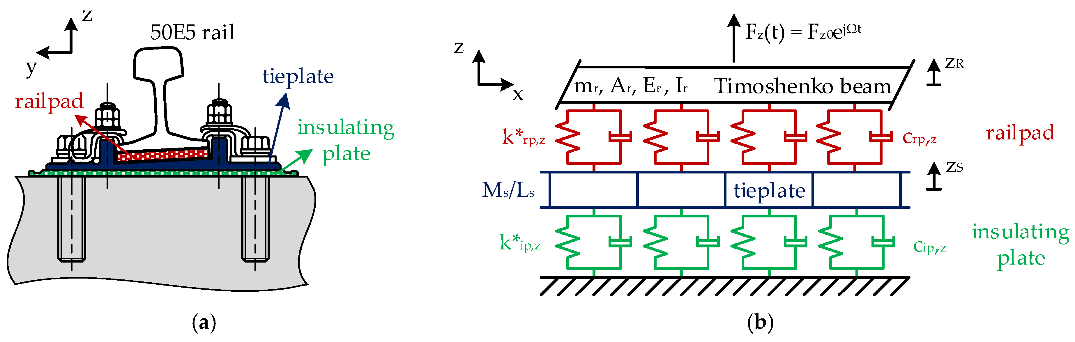
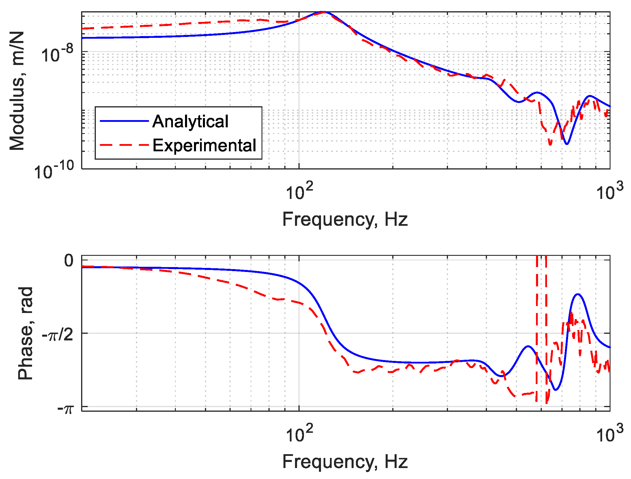
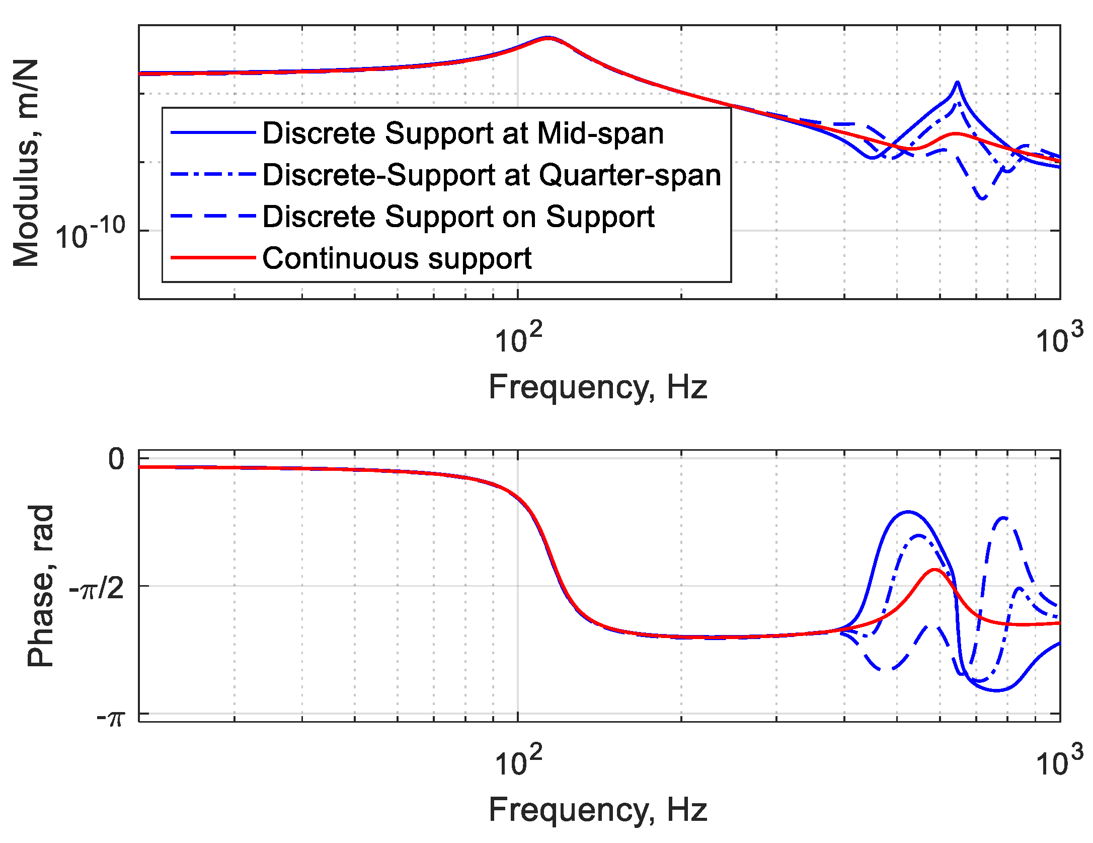
{ x W y W z W } = { x W c y W c z W c } + [ Λ x ] [ Λ y ] [ Λ z ] { 0 0 R w } { 0 0 R w } ,
where
[ Λ x ] = [ 1 0 0 0 1 φ x W a 0 φ x W a 1 ] [ Λ y ] = [ 1 0 φ y W a 0 1 0 φ y W a 0 1 ] [ Λ z ] = [ 1 φ z W a 0 φ z W a 1 0 0 0 1 ] ,
are rotation matrices obtained by considering small displacement assumption and R w is the wheel radius.
The vertical direct receptance A W z ( f ) of the wheel is directly the term z W of Equation (9), since a unit contact force is considered. The comparison between the receptances A W z ( f ) obtained with point mass (dashed blue line) and flexible wheelset (continuous red line) models are shown in Figure 2. Differences between the two models are obviously associated with the presence of resonances in the model accounting for wheelset flexibility. The highly damped resonance peaks at about 6 and 8 Hz are related to the rigid vibration of the wheelset on the primary suspensions, corresponding to the vertical bounce and roll motion, respectively. The peaks at higher frequencies are associated to the flexibility of the wheelset, in particular to its bending modes. Four bending modes are observed in the 0–800 Hz frequency range, whose natural frequencies are 76 Hz, 185 Hz, 370 Hz and 580 Hz.

3.2. Track Dynamics

The trackform present along the analysed section consists of a 50E5 rail (EN 13674-1 [19]) directly fastened to the tunnel. The fastening system is constituted by two elastomeric layers, i.e., the railpad and the insulating plate and a metallic tieplate, as shown in Figure 3a.
With the aim of modelling the infinite nature of the track, a fully analytical model in the vertical plane is used to characterize its behaviour, whose scheme is represented in Figure 3b. The rail is modelled as an infinite Timoshenko beam laying on a double-layer elastic support. The first layer is associated with the flexibility of the railpad, while the second represents the elastomeric insulating plate. The metallic tieplate in between is modelled as a rigid mass. The Timoshenko beam model for the rail is chosen to account for the shear deformation, whose effect becomes more relevant as the frequency increases [20]. The energy dissipation in the elastic layers is introduced using viscous damping elements ( C r p , z and C i p , z ) and loss factors ( η r p and η i p ) to account for the hysteretic behaviour typical of elastomeric materials. The structural damping of the rail η r is considered as a loss factor of 0.02 . The value for the rail is typically smaller, but considering this increased coefficient a better fit agreement with the experimental response of the rail is found. In particular, at high frequencies, the rail foot vibrates at larger amplitudes with respect to the railhead and leads to an increase in the damping effect of the pad [20]. The complex Young’s modulus E r * and shear modulus G r * of the rail become
E r * = E r ( 1 + j η r ) G r * = E r * 2 ( 1 + ν r ) ,
The complex stiffness of the elastomeric elements of the fastening is divided by the fastening spacing L s to calculate stiffnesses per unit length:
k r p z * = K r p , z L s ( 1 + j η r p ) k i p z * = K i p , z L s ( 1 + j η i p ) ,
where K r p , z and K i p , z are the stiffnesses of the railpad and insulating plate, respectively, and L s is the support spacing. The same applies for the viscous damping coefficients. The track data used in the model are summarised in Table 2.
The main assumptions of the analytical model are reported in the following:
  • Displacements are infinitesimally small, to ensure the linearity;
  • The centroid of the beam cross-sections lays on the x-axis, while y- and z-axes are the principal axes of the beam cross-section;
  • The two rails are considered dynamically decoupled;
  • The load applied on the rail is considered fixed in space at x = 0, since the effect of a moving load on the beam dynamics is negligible [21], especially considering the low maximum speeds reached on metro lines;
  • The inclination of the rail is neglected. The load is considered applied in correspondence to the rail neutral axis. This hypothesis allows to decouple the lateral and vertical track dynamics. This is a strong simplification, since the coupling effect increases as the distance along y-axis of the load’s point of application from the neutral axis increases due to the rotation of the rail cross-section.
The system has three degrees of freedom: the rail displacement z R , the rotation of the rail cross-section around the neutral axis ϕ and the tieplate displacement z S . The equations of motion of the system are
{ m r z ¨ R + k e q , z * z R + G r * A r κ r x ( ϕ z R x ) = F z ( t ) δ ( x ) ρ r I r , y y ϕ ¨ E r * I r y y 2 ϕ x 2 + G r * A r κ r ( ϕ z R x ) = 0 ,
where δ ( x ) is the Kronecker delta and k e q z * represents the equivalent dynamic stiffness per unit length of the support, which results in a combination of the railpad and the insulating plate properties:
k e q , z * ( Ω ) = ( k r p , z * + j Ω C r p , z L s ) ( k i p , z * + j Ω C i p z L s Ω 2 M s L s ) k r p , z * + k i p , z * + j Ω ( C r p , z L s + C i p , z L s ) Ω 2 M s L s ,
The analytical expression of the support equivalent stiffness is derived from the equation of motion of the mass representing the tieplate.
The driving point receptance of the rail can be found as the ratio of the displacement of the rail at x = 0 divided by the applied force. The details of the procedure to calculate the track receptance can be found in [20]. The receptance of the track is represented in Figure 4 as a function of the frequency. Three different regions can be distinguished: the first resonance peak around 120 Hz is the resonance of the rail and tieplate vibrating in phase on the insulating plate stiffness. The other peak around 680 Hz corresponds to the resonance of the rail vibrating in anti-phase with the tieplate on the stiffness of the rail-pad. In correspondence with the anti-resonance at about 530 Hz the rail is stationary, while the plate vibrates between the two layers of stiffness, acting as a vibration absorber.
The analytical receptance of the analysed track section is compared in Figure 5 with the experimental one in order to verify the accuracy of the analytical model. The experimental receptance is obtained by means of a hammer test, in which the rail is excited with an impulse force. The direct response of the rail is measured using an accelerometer positioned as close as possible to the excitation point. The trend of the analytical model correctly reproduces the real behaviour of the track in the frequency band of interest. In the validation phase, discrete supports are considered in the analytical model. The direct receptances in Figure 5 are obtained in correspondence with a support. The anti-resonance at 650 Hz is due to the pinned-pinned resonance of the track.
Once the support parameters (listed in Table 2) are calibrated on the basis of the experimental data, an equivalent continuously supported track is considered on account of the fact that the variability of track receptance along the span cannot be considered in the present linearised model of the wheel–rail interaction. Figure 6 shows the comparison between the direct receptances calculated with the discrete supports using different excitation points and the one obtained by using the continuous support. In the frequency range of interest, the differences between the results using the two different approaches are negligible.

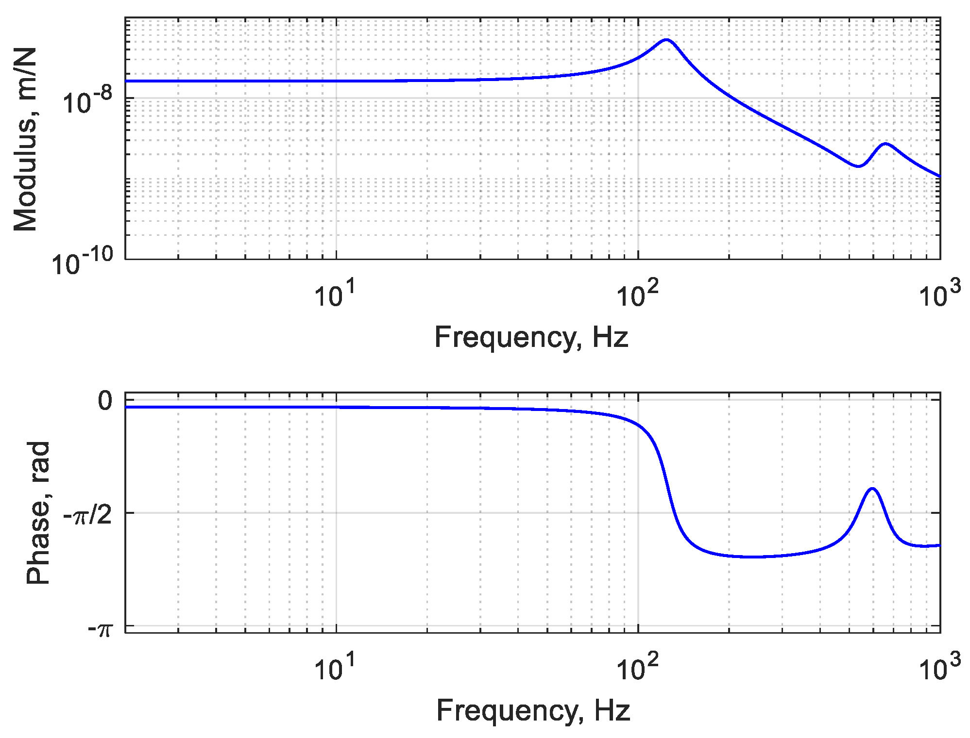
3.3. Dynamics of the Wheel–Rail Coupled System

The vertical dynamics of the wheel–rail interaction can be studied using the scheme represented in Figure 7.
As already said, the irregularity of the rail surface is considered as a harmonic excitation which causes fluctuations in the contact parameters around their reference value, indicated with Δ . The displacements are taken positive when upwards, while the force exchanged between the wheel and the rail is taken positive, as represented in Figure 7. The Hertzian contact stiffness k H allows to model the local deformability of the wheel and the rail. Its value is considered constant with frequency and equal to 1.2 GN/m.
The compression of the contact spring δ can be expressed as follows:
δ = Δ z R + z i r r Δ z W ,
where Δ z W and Δ z R are the fluctuations in the displacement of the contact point on the wheel and the rail, respectively, induced from the rail irregularity z i r r . The compression of the Hertzian contact spring is always positive since it works only in compression. It can be expressed as follows:
δ = Δ F z k H ,
The fluctuations in the contact point displacements are calculated by considering wheel and rail direct receptances:
Δ z W = A W z ( f ) Δ F z Δ z R = A R z ( f ) ( Δ F z ) ,
The minus in the expression of Δ z R is related to the fact that the receptance of the rail is calculated considering force and displacement positive when directed in the same direction, while in the notation of Figure 7 these are opposite. By substituting Equations (16) and (17) into Equation (15), the irregularity on the rail can be written as
z i r r = ( A W z ( f ) + A R z ( f ) + 1 k H ) Δ F Z = T ( f ) Δ F z ,
The transfer function T ( f ) represents the ratio between the rail irregularity and the induced fluctuation in the vertical contact force, i.e., the vertical receptance of the coupled wheel–rail system. It is obtained as the sum of three components according to Equation (18): the direct receptances of wheel, rail and Hertzian spring. The transfer function T ( f ) derived with the point mass and deformable wheelset model are shown in Figure 8a,b, respectively. In the figures, the single components are also shown. At low frequencies, the dynamics of the wheel–rail interaction is mainly determined by the dynamics of the wheelset, while the track dynamics governs the high-frequency behaviour. The receptances of the coupled system derived with the two wheelset models present a similar trend since they are in the 20–50 Hz frequency range, where the wheelset dynamics is dominant. In the frequency range of interest for this problem, the effect of the contact stiffness is negligible. When higher frequencies are involved, the effect of the contact stiffness becomes more relevant, and also the effect of the contact filter effect should be considered [22,23].
The equations written above are valid for both point mass and flexible wheelset models. They differ only in the analytical expression of A W z ( f ) . The main difference between the two approaches is in the calculation of the transfer function between the vertical axlebox acceleration and the fluctuation in the vertical contact force. It can be calculated as the double derivative of the axlebox displacement with respect to time. When the point mass wheel model is used, the axlebox acceleration is equal to the one of the wheel centres and can be calculated by using Newton’s second law:
z ¨ a x = Δ F z M w ,
On the other hand, if the flexible wheelset model is considered, the cross-receptance A B z ( f ) representing the axlebox vertical displacement per unit contact force is used. It is derived by the modal model of the wheelset. Thus, the axlebox acceleration takes the following form:
z ¨ a x = ( 2 π f ) 2 A B z ( f ) Δ F z ,
Thus, the transfer function H ( f ) of the axlebox measurement system is calculated with the point mass and flexible wheelset approaches by combining Equation (18) with Equations (19) and (20), respectively. The point mass wheelset model is expressed by the following relationship:
H p m ( f ) = M w T ( f ) ,
while for the flexible wheelset model it becomes
H d w ( f ) = z i r r z ¨ a x = T ( f ) ( 2 π f ) 2 A B z ( f ) ,
The transfer functions obtained with the two approaches are compared in Figure 9. When the wheel is modelled as a point mass the transfer function of the system is mainly determined by the track dynamics, since the wheelset dynamics is completely neglected. On the other hand, the modal model of the wheelset allows to consider its flexibility in the calculation of the axlebox acceleration.
In general, at frequencies below 50 Hz the two approaches lead to a similar behaviour of transfer response, since the overall dynamics is determined by the wheelset mass. As the frequency increases, the point mass wheel model leads to a global overestimation of the irregularity except at specific frequencies that correspond to the resonances of the wheelset, where an underestimation occurs. In particular, this happens in correspondence to the peaks at about 70 Hz (first bending mode of the wheelset) and at 190 Hz (second bending mode). The difference between the two approaches arises from the calculation of the axlebox acceleration. When the deformable wheelset is considered, the axlebox acceleration is derived considering the wheelset dynamics (term A B z ( f ) of Equation (20)). On the other hand, when the wheelset is modelled as a point mass, the axlebox acceleration is related to the vertical force fluctuation by Newton’s second law (Equation (19)).
The overestimation is due to the fact that part of the energy introduced by the irregularity is dissipated by the wheelset flexibility, which is completely neglected in the point mass wheel model. The assumption of the point mass wheel model is a good approximation if the travelling speed of the vehicle and the consequent excitation frequency induced by the rail irregularity (Equation (3)) are sufficiently low. As the speed increases, this assumption is less valid. It is also worth mentioning that the underestimation of the irregularity at frequencies corresponding to wheelset modes can lead to errors in monitoring rail corrugation. In fact, it is common that that corrugation tends to form at wavelengths related to the frequencies of wheelset modes.
The transfer function is calculated considering the dynamics of a specific track section, but the approach is general. If the receptances of all the different trackforms present along the line are known, they can be substituted in Equation (18) to obtain the corresponding transfer function of the measurement system, allowing rail corrugation monitoring along the entire line.

4. Algorithm for Rail Irregularity Estimation
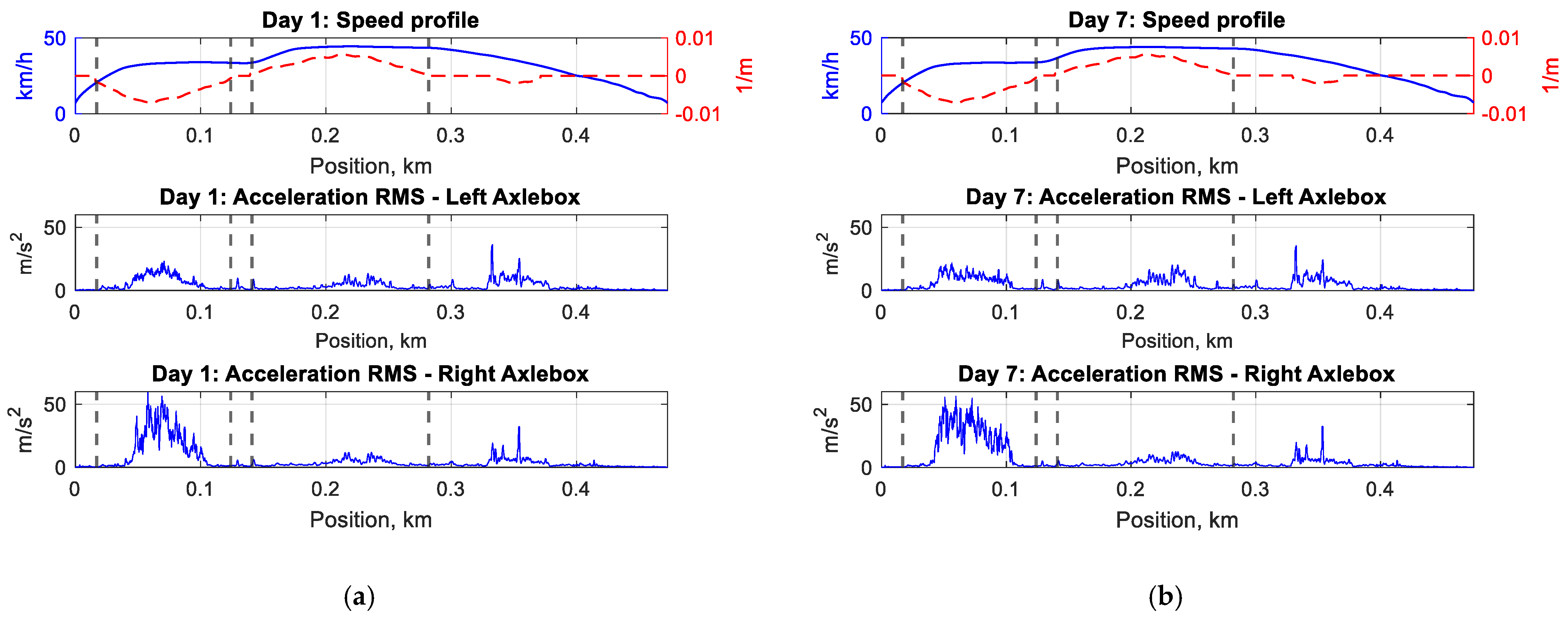
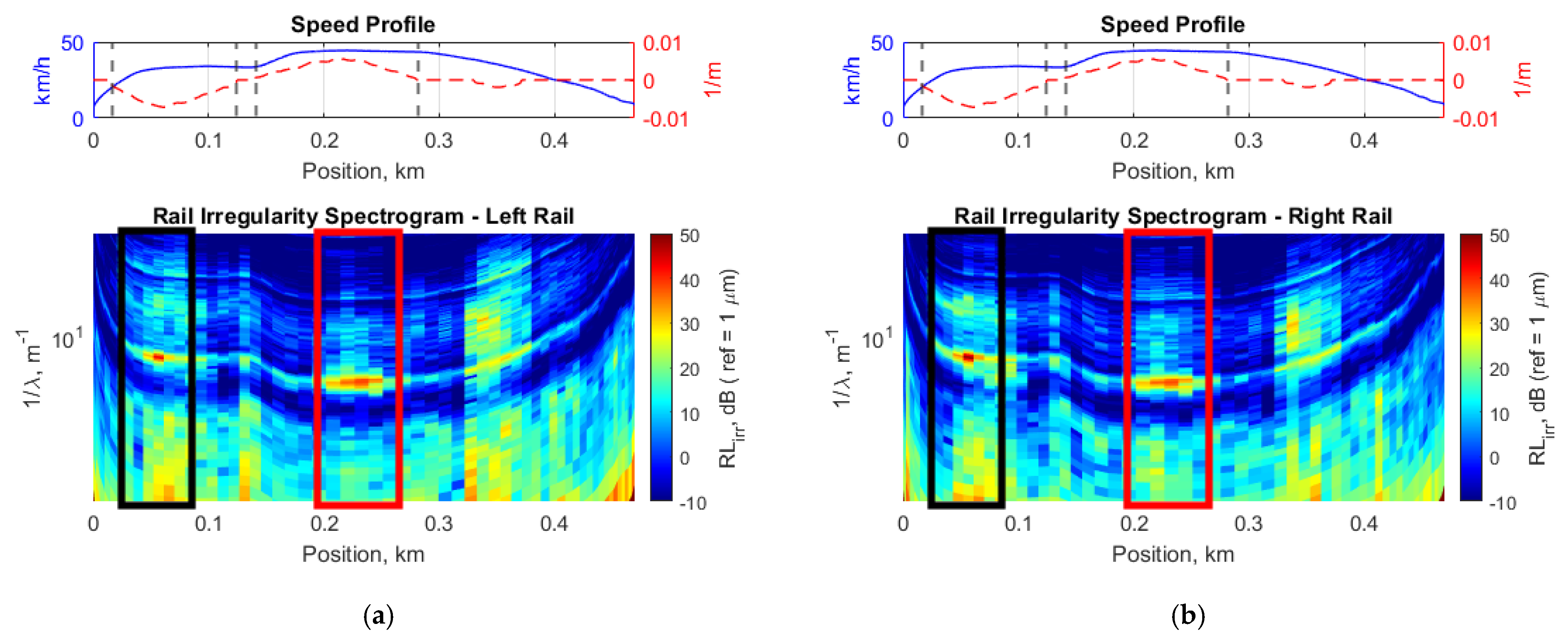
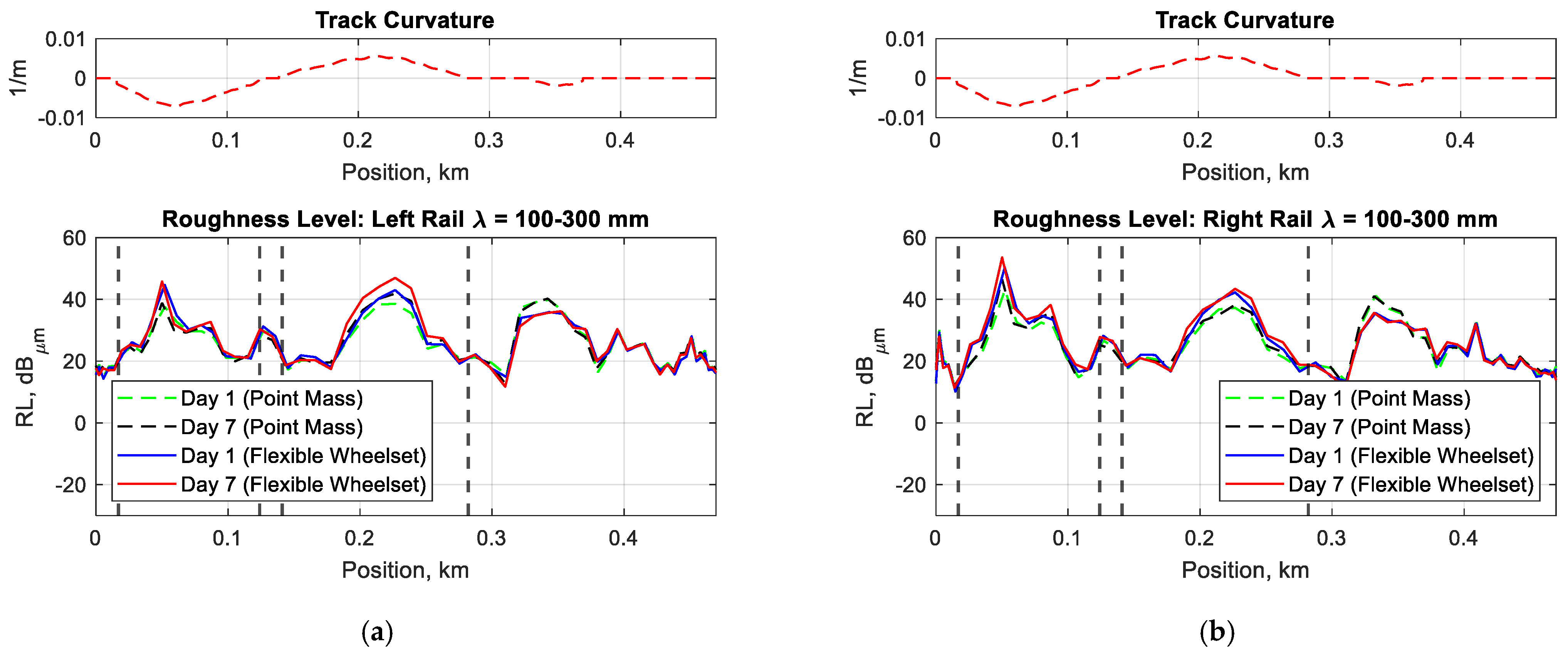
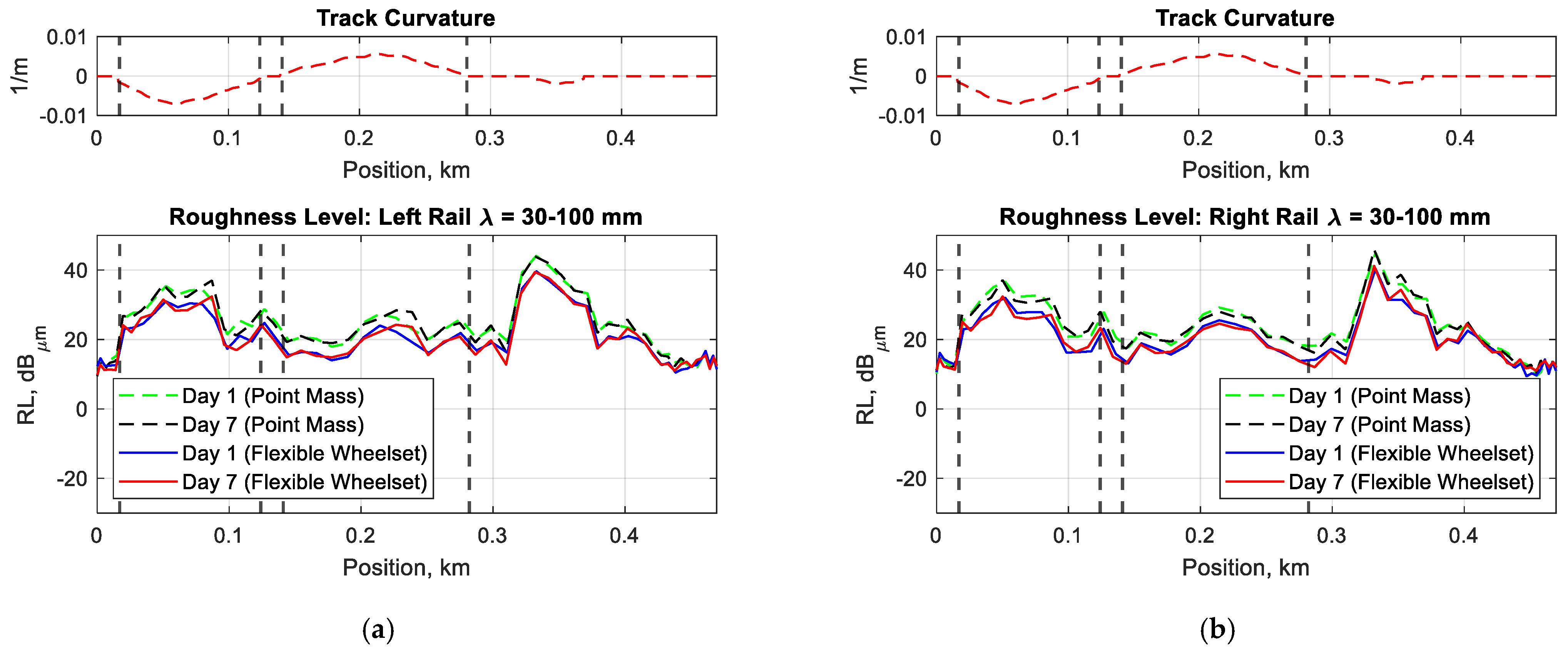
After the calculation of the transfer function of the axlebox acceleration measurement system, an algorithm for rail roughness estimation is proposed, which is based on the calculation of the power spectrum of the rail irregularity.
To this aim, the acceleration signals are divided into independent time bins of duration T b i n . The power spectrum of the acceleration signal within the k -th time bins is estimated using the Welch method [24], in order to reduce the effect of noise on the acceleration measurements. The time bin is sub-divided into sub-windows of duration T w i n < T b i n . A user-defined overlap of the sub-windows (of time T o v e r ) is used. A Hanning window function is applied to the sub-windows, in order to force the signal to be periodic. Finally, the power spectrum P a c c , k ( f ) in the k -th time bin is calculated by averaging the power spectra of the sub-windows.
As a general comment, the proposed methodology is needed on account of the fact that acceleration data cannot be compared directly, because they are not always acquired at the same speed.
The power spectra are in the frequency domain, but they can be expressed in the wavelength domain thanks to the speed signal measured with the encoder. In particular, the average speed in each time bin is used to switch from frequency to wavelength by means of Equation (3). By approximating the speed in the time bin as constant, a small error is committed when switching from the frequency to the wavelength domain. The lower the length of time bins T b i n the lower the error. However, shorter time bins make the power spectra more sensible for finding local defects on the rail.
Another important parameter of the algorithm is the length of the sub-windows T w i n used for the estimation of the power spectra of the acceleration signal. The shorter the sub-windows the higher the number of power spectra used in the averaging operation, and thus the higher the filtering of noise that affects the measurements. However, having short sub-windows leads to a low-frequency resolution. A trade-off between the frequency resolution and the noise filtering is found. The parameters used in the estimation of the irregularity power spectra are listed in Table 3, which are selected in order to find a compromise among the aforementioned aspects.
The power spectra of the rail irregularities are calculated by considering the transfer function H i ( f ) of the axlebox accelerometer measurement system:
P i r r , k ( f ) = | H i ( f ) | 2 P a c c , k ( f ) ,

5. Results

The two approaches presented in this paper are compared by considering two different runs of the instrumented vehicle on a single track section between two stations. The second run is performed six days after the first. On the analysed site two curves are present: the first is a right curve (radius of 133 m) and the second is a left curve (radius of 173 m). It is known that corrugation appears on the low rail of both the curves.
The data relative to Day 1 are shown in Figure 10a, while Figure 10b refers to the data acquired on Day 7. The curves are highlighted by vertical dashed lines for a better understanding. All the data are represented as a function of the position of the leading wheelset of the train on the line, measured in kilometres. In the upper plot the vehicle speed profile (solid line) and the estimated horizontal curvature of the track (dashed line) are represented. The latter is equal to the inverse of the curve radius and it is obtained from the combination of the signal by the gyroscope mounted on the carbody with the vehicle speed. If this quantity is equal to zero the vehicle is running on a straight track, if it is positive the train is negotiating a left curve, while if it is negative the train is negotiating a right curve. The moving rms of the acceleration measured at the axleboxes of the leading wheelset of the instrumented bogie are shown in the lower plots.
At about km 0.32 there is a switch, responsible for the high rms levels. A high acceleration is experienced by the right axlebox in correspondence to the first right curve (from km 0.02 to km 0.12). This may indicate the presence of a severe corrugation on the low (inner) rail. When the vehicle is negotiating the second left curve (from km 0.14 to km 0.28), there is an increase in the rms level relative to the left axlebox accelerometer from Day 1 to Day 7. This increment may be related to the rapid development of rail corrugation on the low rail of the curve.
The power content of the rail irregularity is estimated in terms of Roughness Level (RL) as a function of the wavelength of the irregularity, which is defined by EN ISO 3095 [25] as
R L ( 1 λ ) = 10 log 10 ( P i r r ( 1   λ ) r 0 2 )                                       r 0 = 1   μ m ,
As an example, the spectrograms of the estimated rail irregularity (by using the flexible wheelset approach) relative to Day 1 are shown in Figure 11. The spectrogram represents the Roughness Level (colormap) as a function of the wavelength (y-axis) and the absolute position of the wheelset along the line (x-axis). In correspondence to the two curves, the rails manifest a high RL restricted to a narrow wavelength band, indicating the presence of rail corrugation, which is almost mono-harmonic, with a wavelength of about 130 mm in the first right curve (highlighted in black) and a 170 mm wavelength in the second left curve (highlighted in red). In-field observations show that on both the curves rail corrugation tends to develop on the low rail. From the spectrogram, it is not clear which rail shows corrugation, since a high RL is present on both of them. The reason is that in the model of the vertical dynamics of the wheel–rail interaction the two sides of the wheelset are considered dynamically decoupled. Actually, the irregularity on a rail generates vibrations also measured by the accelerometer placed on the axlebox on the opposite side. Thus, a more sophisticated model that considers this coupling effect will allow to better identify which rail is corrugated.
Rail corrugation monitoring is performed by computing the RL within the four wavelength bands prescribed by EN 13231-3 [26], which defines the acceptance criteria for the grinding operations on the rail running surface. The wavelength bands are 10–30 mm, 30–100 mm, 100–300 mm and 300–1000 mm. Attention has been paid only to the 30–100 mm and 100–300 mm wavelength bands, where corrugation is typically found in the specific line.
The RLs in 100–300 mm and 30–100 mm bands are shown for the considered runs in Figure 12 and Figure 13, respectively. The curves of the track section under analysis are highlighted in the figures by vertical dashed lines for a better understanding.
By looking at the RL in the 100–300 mm wavelength band, the highest RL values are observed on the low rail of the curves (Figure 12b for the second curve). This is in accordance with the spectrograms of Figure 11: they indicate a corrugation wavelength of 130 mm on the first curve and a 170 mm corrugation wavelength on the second one. The average speed on the first right curve is about 33 km/h, while the second one is negotiated at an average speed of 43 km/h (Figure 10). Thus, for both the curves, the frequency of excitation by the rail irregularity is about 70 Hz according to Equation (3), which corresponds to the natural frequency of the first bending mode of the wheelset. On account of the differences in the transfer functions reported in Figure 9 at the same frequency, the RL on the low rail estimated with the flexible wheelset model is 7 dB higher than the one predicted with the point mass model. The same difference is observed both on Day 1 and Day 7. This indicates that the transfer function calculated with the flexible wheelset model is more sensible for finding the presence of rail corrugation and therefore the proposed approach will be more effective for its monitoring.
The RL on the high rail is lower with respect to the low rail, but its absolute value is in any case significant. As mentioned before, this is related to the fact that the two axleboxes of the wheelset are not dynamically decoupled, and thus both axlebox accelerometers are measuring vibrations at the excitation frequency defined by the corrugation wavelength. The low rail of the second left curve shows a significant increment in the RL of about 5 dB from Day 1 to Day 7, indicating that the corrugation growth rate is high and attention should be paid in the scheduling of rail grinding operations.
Concerning the 30–100 mm wavelength band, the RL on the two rails shows a minor variation in the considered time interval. This is consistent with the fact that no corrugation is observed within this wavelength band. As anticipated in Section 3.3, the transfer function of the measurement system using the point mass model overestimates the rail irregularity in the medium-to-high frequency range, expected at the wheelset natural frequencies (Figure 9). The 30–100 mm wavelength band corresponds to the 90–300 Hz frequency range for the first curve (negotiated at 33 km/h) and to the 120–400 Hz range for the second one (negotiated at 43 km/h).

6. Conclusions

A procedure for the continuous monitoring of rail corrugation along a metro line has been proposed. It is based on acceleration measurements performed by axlebox accelerometers mounted on a commercial vehicle.
A single vehicle equipped with this measurement system allows to collect data on the rail conditions along the whole line several times per day. The output of the monitoring system is the estimate of the power spectra of rail irregularity. This helps in promptly identifying specific locations where corrugation is developing and to schedule rail grinding operations only when and where they are strictly necessary.
The estimation of the rail roughness from axlebox acceleration measurements requires the knowledge of the transfer function of the measurement system, which relates the input rail irregularity to the measured acceleration. It was calculated by studying the vertical dynamics of the wheel–rail interaction with a linearised model in the frequency domain. Two different approaches for the characterisation of the wheel dynamics have been proposed. The first state-of-the-art approach is used in the HRSCA measurement system and considers the wheel as a point mass, while in the proposed methodology the dynamic behaviour of the wheel is derived by considering the wheelset as a flexible body. The track dynamics is characterised by using an analytical model validated experimentally.
The transfer functions calculated with the two approaches are similar at low frequencies, at which the dynamics of the wheel–rail interaction is mainly determined by the wheel mass, and therefore the point mass assumption is reasonable. At higher frequencies, the track dynamics becomes predominant, and neglecting the wheelset flexibility leads to an overestimation of the rail irregularity. In this frequency range the transfer function derived with the flexible wheelset model amplifies the irregularity at the natural frequencies of its mode shapes. This eases the identification of the corrugated track section, since it is common that corrugation tends to form at wavelengths related to the natural frequencies of the wheelset by the vehicle speed.
The transfer functions of the HRSCA measurement system and of the proposed one were used to estimate the power spectrum of rail irregularity in terms of Roughness Level (within the 30–100 mm and 100–300 mm wavelength bands of Standard EN 13231-3) on a track section of a subway line between two stations. The results indicate the presence of corrugation on the low rail of both the curves in the 100–300 mm wavelength band, which was confirmed by in-field observations. The flexible wheelset model shows a higher RL in the 100–300 mm wavelength band with respect to the point mass mode, indicating that the proposed measurement system is more sensible for finding the presence of rail corrugation. Moreover, a fast corrugation development is observed on the low rail of a curve of the analysed site. On the contrary, in the 30–100 mm wavelength band, in which no corrugation is observed, the point mass model leads to an overestimation of the RL with respect to that proposed along the whole track section.
The proposed methodology can be used for the continuous monitoring of rail corrugation at service speed, and it is effective in identifying those sections where corrugation is developing and rail grinding becomes necessary. However, a relatively high Roughness Level is also estimated on the high rail of the corrugated curves. This is related to the fact that the axleboxes of the same wheelset are assumed to be dynamically decoupled. This is a strong assumption because the irregularity of a rail induces wheelset vibrations that are also measured by sensors on the opposite side. A more refined model of the wheel–rail interaction that considers this dynamic coupling is needed for a more accurate estimation.

Author Contributions

Conceptualization, E.D.G. and C.S.; methodology, L.F. and J.K.; software, L.F. and J.K.; validation, L.F., J.K., E.D.G. and C.S.; formal analysis, L.F. and J.K.; investigation, L.F. and J.K.; resources, E.D.G. and C.S.; data curation, J.K.; writing—original draft preparation, L.F.; writing—review and editing, L.F. and E.D.G.; visualization, L.F.; supervision, E.D.G. and C.S.; project administration, M.B. and A.C.; funding acquisition, M.B. and A.C. All authors have read and agreed to the published version of the manuscript.

Funding

This research received no external funding.

Institutional Review Board Statement

Not applicable.

Informed Consent Statement

Not applicable.

Data Availability Statement

Data is unavailable due to privacy.

Acknowledgments

The authors are grateful to Azienda Trasporti Milanesi S.p.A for supporting the research and providing the possibility to perform experimental tests on the track and to use data from the instrumented vehicle.

Conflicts of Interest

The authors declare no conflict of interest.

References

  1. Grassie, S.L. Corrugation on Australian National: Cause, Measurement and Rectification. In Proceedings of the 4th International Heavy Haul Railway Conference, Brisbane, Australia, 1 January 1989; pp. 188–192. [Google Scholar]
  2. Tassilly, E.; Vincent, N. Rail Corrugations: Analytical Model and Field Tests. Wear 1991, 144, 163–178. [Google Scholar] [CrossRef]
  3. Grassie, S.L. The Corrugation of Railway Rails: 1. Introduction and Mitigation Measures. Proc. Inst. Mech. Eng. F J. Rail Rapid Transit. 2022, 2022, 095440972211256. [Google Scholar] [CrossRef]
  4. Grassie, S.L.; Kalousek, J. Rail Corrugation: Characteristics, Causes and Treatments. Proc. Inst. Mech. Eng. F J. Rail Rapid Transit. 1993, 207, 57–68. [Google Scholar] [CrossRef]
  5. Grassie, S.L. Rail Corrugation: Characteristics, Causes, and Treatments. Proc. Inst. Mech. Eng. F J. Rail Rapid Transit. 2009, 223, 581–596. [Google Scholar] [CrossRef]
  6. Grassie, S.L. The Corrugation of Railway Rails: 2. Monitoring and Conclusions. Proc. Inst. Mech. Eng. F J. Rail Rapid Transit. 2022, 2022, 09544097221122011. [Google Scholar] [CrossRef]
  7. Grassie, S.L. Measurement of Railhead Longitudinal Profiles: A Comparison of Different Techniques. Wear 1996, 191, 245–251. [Google Scholar] [CrossRef]
  8. Mauz, F.; Wigger, R.; Wahl, T.; Kuffa, M.; Wegener, K. Acoustic Roughness Measurement of Railway Tracks: Implementation of a Chord-Based Optical Measurement System on a Train. Appl. Sci. 2022, 12, 11988. [Google Scholar] [CrossRef]
  9. Tufano, A.R.; Chiello, O.; Pallas, M.A.; Faure, B.; Chaufour, C.; Reynaud, E.; Vincent, N. Numerical and Experimental Analysis of Transfer Functions for On-Board Indirect Measurements of Rail Acoustic Roughness. Notes Numer. Fluid. Mech. Multidiscip. Des. 2021, 150, 295–302. [Google Scholar] [CrossRef]
  10. Pieringer, A.; Kropp, W. Model-Based Estimation of Rail Roughness from Axle Box Acceleration. Appl. Acoust. 2022, 193, 108760. [Google Scholar] [CrossRef]
  11. Grassie, S.L. Measurement of Longitudinal Irregularities on Rails Using an Axlebox Accelerometer System. Notes Numer. Fluid. Mech. Multidiscip. Des. 2021, 150, 320–328. [Google Scholar] [CrossRef]
  12. Frederick, C.O. A Rail Corrugation Theory. In Contact Mechanics and Wear of Rail/Wheel. Systems II; University of Waterloo Press: Waterloo, ON, Canada, 1986; Volume 2, pp. 181–211. [Google Scholar]
  13. Tassilly, E.; Vincent, N. A Linear Model for the Corrugation of Rails. J. Sound. Vib. 1991, 150, 25–45. [Google Scholar] [CrossRef]
  14. Hempelmann, K.; Knothe, K. An Extended Linear Model for the Prediction of Short Pitch Corrugation. Wear 1996, 191, 161–169. [Google Scholar] [CrossRef]
  15. Muller, S. A Linear Wheel-Rail Model to Investigate Stability and Corrugation on Straight Track. Wear 2000, 243, 122–132. [Google Scholar] [CrossRef]
  16. Knothe, K. Non-Steady State Rolling Contact and Corrugations. In Rolling Contact Phenomena; Springer: Wien, Austria, 2000; pp. 203–276. [Google Scholar]
  17. Baeza, L.; Fayos, J.; Roda, A.; Insa, R. High Frequency Railway Vehicle-Track Dynamics through Flexible Rotating Wheelsets. Veh. Syst. Dyn. 2008, 46, 647–659. [Google Scholar] [CrossRef]
  18. Martínez-Casas, J.; Di Gialleonardo, E.; Bruni, S.; Baeza, L. A Comprehensive Model of the Railway Wheelset-Track Interaction in Curves. J. Sound. Vib. 2014, 333, 4152–4169. [Google Scholar] [CrossRef] [Green Version]
  19. EN 13674-1:2011; Railway Applications-Track-Rail Part. 1: Vignole Railway Rails 46 Kg/m and above. British Standard Institution: London, UK, 2011.
  20. Thompson, D. Railway Noise and Vibration: Mechanisms, Modelling and Means of Control, 1st ed.; Elsevier Ltd.: Oxford, UK, 2009; ISBN 9780080451473. [Google Scholar]
  21. Grassie, S.L.; Gregory, R.W.; Harrison, D.; Johnson, K.L. Dynamic Response of Railway Track to High Frequency Vertical Excitation. J. Mech. Eng. Sci. 1982, 24, 77–90. [Google Scholar] [CrossRef]
  22. Remington, P.; Webb, J. Estimation of Wheel/Rail Interaction Forces in the Contact Area Due to Roughness. J. Sound. Vib. 1996, 193, 83–102. [Google Scholar] [CrossRef]
  23. Bellette, P.A.; Meehan, P.A.; Daniel, W.J.T. Contact Induced Wear Filtering and Its Influence on Corrugation Growth. Wear 2010, 268, 1320–1328. [Google Scholar] [CrossRef]
  24. Welch, P.D. The Use of Fast Fourier Transform for the Estimation of Power Spectra: A Method Based on Time Averaging over Short, Modified Periodograms. IEEE Trans. Audio Electroacoust. 1967, 15, 70–73. [Google Scholar] [CrossRef] [Green Version]
  25. EN ISO 3095:2013; Acoustics-Railway Applications-Measurement of Noise Emitted by Railbound Vehicles. British Standard Institution: London, UK, 2013.
  26. EN 13231-3:2012; Railway Applications-Track-Acceptance of Works-Part. 3: Acceptance of Reprofiling Rails in Track. British Standard Institution: London, UK, 2012.
Figure 1. Accelerometers mounted on the axlebox of a wheelset of the instrumented trailer bogie (the same setup is repeated on the other wheelset): (a) side A, vertical axlebox accelerometer; (b) side B, vertical and lateral axlebox accelerometers.
Applsci 13 03773 g001
Figure 2. Direct vertical receptance of the wheel derived with point mass and flexible wheelset model.
Applsci 13 03773 g002
Figure 3. (a) Direct fastening system installed on the analysed track section; (b) scheme of the analytical track model. The explanation of * is given in Equation (12).
Applsci 13 03773 g003
Figure 4. Track direct vertical receptance.
Applsci 13 03773 g004
Figure 5. Analytical and experimental direct vertical receptance of the tested track in correspondence with a support.
Applsci 13 03773 g005
Figure 6. Analytical direct receptance calculated with discretely and continuously supported track. When discrete supports are considered, the receptance is calculated at different positions along the span between two supports.
Applsci 13 03773 g006
Figure 7. Scheme of the vertical wheel–rail interaction.
Applsci 13 03773 g007
Figure 8. Wheel, track, Hertzian spring and coupled wheel–rail system direct vertical receptances: (a) considering the wheelset as a point mass; (b) considering the deformable wheelset model.
Applsci 13 03773 g008
Figure 9. Transfer functions of the axlebox acceleration measurement system, derived with point mass and flexible wheelset models.
Applsci 13 03773 g009
Figure 10. Speed profile and moving rms of the vertical acceleration measured at the axleboxes of the leading wheelset of the instrumented bogie: (a) day 1; (b) day 7.
Applsci 13 03773 g010
Figure 11. Spectrogram of the rail irregularity on Day 1, along with the vehicle speed (solid line) and the horizontal curvature of the track (dashed line): (a) left rail; (b) right rail.
Applsci 13 03773 g011
Figure 12. Roughness Level in the 100–300 mm wavelength band: (a) left rail; (b) right rail.
Applsci 13 03773 g012
Figure 13. Roughness Level in the 30–100 mm wavelength band: (a) left rail; (b) right rail.
Applsci 13 03773 g013
Table 1. Wheelset data and list of symbols.
ParameterSymbolValue
Wheelset mass M w h 1054 kg
Axle mass M a x l e 283 kg
Axlebox mass M a x 78 kg
Wheel mass M w h e e l 251 kg
Brake disk mass M b r a k e 135 kg
Primary suspension stiffness (vertical) k p s , z 2 × 0.5 kN / mm
Primary suspension stiffness (lateral) k p s , y 2 × 2.1 kN / mm
Primary suspension stiffness (longitudinal) k p s , x 2 × 4.15 kN / mm
Primary suspension damping (vertical) c p s , z 11 kNs / m
Primary suspension damping (lateral) c p s , y 50 kNs / m
Primary suspension damping (longitudinal) c p s , x 85 kNs / m
Wheel nominal radius R w h e e l 0.41 m
Point mass M w 605 kg
Table 2. Track data and list of symbols.
ParameterSymbolValue
Rail mass (unit length) m r 49.9 kg / m
Rail cross-section A r 63.62 cm 2
Rail moment of inertia (y-y) I r , y y 1844 cm 4
Rail Young Modulus E r 2.06 × 10⁵  MPa
Poisson ratio   ν r 0.28
Rail shear factor κ r 0.34
Rail loss factor η r 0.02
Support spacing L s 0.75 m
Railpad stiffness K r p , z 150 kN / mm
Railpad loss factor η r p , z 0.13
Railpad viscous damping C r p , z 1.5 kNs / m
Tieplate mass M s 15 kg
Ins. plate stiffness K i p , z 30 kN / mm
Ins. plate loss factor η i p , z 0.20
Ins. plate viscous damping C i p , z 2.8 kNs / m
Table 3. Parameters used in the algorithm for the estimation of the power spectrum of rail irregularity.
ParameterSymbolValue (s)
Time bin duration T b i n 1
Sub-window duration T w i n 0.5
Overlapping time T o v e r 0.25
Disclaimer/Publisher’s Note: The statements, opinions and data contained in all publications are solely those of the individual author(s) and contributor(s) and not of MDPI and/or the editor(s). MDPI and/or the editor(s) disclaim responsibility for any injury to people or property resulting from any ideas, methods, instructions or products referred to in the content.

