Adaptive Suppression Method of LiDAR Background Noise Based on Threshold Detection

Abstract

Background radiation in the LiDAR detection field of view is complex and variable, and the background noise generated can easily cause false alarms in the receiver, which affects the effective detection of the system. Through the analysis of the influence of background radiation noise of LiDAR on the detection performance, an adaptive suppression method of LiDAR background noise is proposed. This method realizes the rapid suppression of background noise in the instantaneous field of view through an adaptive threshold adjustment of current steering architecture with a back-end digital-to-analog converter (DAC) correction based on the principle of constant false alarm rate (CFAR) control. Aiming at the problem of accurate noise detection and quantification in a very short time, a dynamic comparator is used to replace the traditional continuous comparator. While detecting the number of noise pulses, the measurement of the pulse duration of noise is realized, which improves the accuracy of short-time noise detection. In order to verify the actual effect of the adaptive method, experiments were carried out based on the team’s self-developed LiDAR. The experimental results show that the measured noise ratio of the adaptive mode by using this method is the lowest. Even at 12 a.m., the noise ratio of the point cloud obtained by the adaptive mode is 0.012%, compared with 0.08% obtained by the traditional mode, which proves that this method has a good ability to suppress background noise. The proportion of noise reduction of the adaptive mode is more than 80% compared with the traditional mode. It achieves noise suppression through hardware at each detection, and each adjustment can be completed within a single period of pulse detection. Therefore, it has great advantages in real-time detection compared with the back-end software noise reduction processing method, and it is suitable for the application of LiDAR in the complex background environment.

1. Introduction

LiDAR has developed rapidly since the creation of lasers, and pulsed LiDAR obtains the distance of target objects by the time of flight (TOF) method, which has the characteristics of a simple detection method, long distance, and high efficiency [1,2,3], and has wide applications in the fields of target reconnaissance, navigation, surveying and mapping [4,5,6]. With the improvement in performance requirements for applications in various fields, miniaturization, high adaptability and reliability have become important development directions for LiDAR technology [7,8], which has higher demands for the front-end receiving system of LiDAR. With strong background radiation, the background environment in the instantaneous receiving field of view is complex and changeable, so that the background noise power received by the system also changes accordingly, which is easy to appear as a “false alarm” during signal detection, thus increasing the burden of signal processing, leading to the reduction in the point cloud signal-to-noise ratio (SNR), and in serious cases, the system cannot work normally [9]. Therefore, the receiver system needs to be able to be adjustable to the changes in background radiation in order to suppress the noise and thus improve LIDAR interference immunity and environmental adaptability. Common methods to suppress background radiation noise include the field-of-view method [10], spectrum filtering method [11], video bandwidth method [12], time discrimination method [13], time program gain method [14], polarization identification method [15], CFAR control method [16] and logic resolution method [17]. Among them, the method of adjusting the circuit performance parameters in LiDAR to suppress the background radiation noise is relatively simple, particularly the CFAR control method, which is used to control the FAR of the system by adjusting the receiver circuit parameters according to the noise detection in the receiver, and which can effectively suppress the false alarm interference caused by the background radiation.

In the published reports and literature, there has been much research on the influence of background radiation noise on the detection performance of LiDAR and the adjustment and suppression methods [18,19]. Based on the characteristics of the avalanche photodiode (APD) optoelectronic receiver system, the FAR Gaussian model was modified to improve the model accuracy at higher temperatures and avalanche gain effectively [20]. The relationship between background radiation and multiplication factors of APD was modeled by studying the effect of background radiation on APD detection performance, combined with the principle of CFAR compensation [21]. Aiming at the background radiation noise and multiplication characteristics of APD, the study of an adaptive bias control method was carried out [22]. According to the different background radiation levels, a CFAR control technique is proposed based on FPGA in LiDAR [23].

Most research focuses on the method of changing the operating voltage of APD, which is equivalent to adjusting the APD multiplier, for background radiation noise suppression, but these methods have a low response speed of adjustment due to the bandwidth limitation of the high voltage source of APD so that they cannot be quickly adjusted according to the background radiation changes in the instantaneous field of view when the laser radar is scanning the large field of view. In this paper, the influence of background radiation noise of LiDAR on the detection performance is analyzed, the principle of CFAR and the implementation method of threshold control are studied, and then an adaptive suppression method of background radiation noise of LiDAR through threshold adjustment is proposed. Based on the traditional adjustment mode, the signal identification threshold is automatically adjusted by the cascade current steering architecture with a back-end digital-to-analog converter (DAC) correction to achieve CFAR control of LiDAR. In order to solve the problem of quantization deviation of a short time in noise detection, a dynamic comparator is used to replace the traditional continuous comparator, and the comparator implementation structure and threshold selection requirements are studied. Finally, comparative experiments are carried out by using this method on LiDAR, and the experimental results are analyzed.

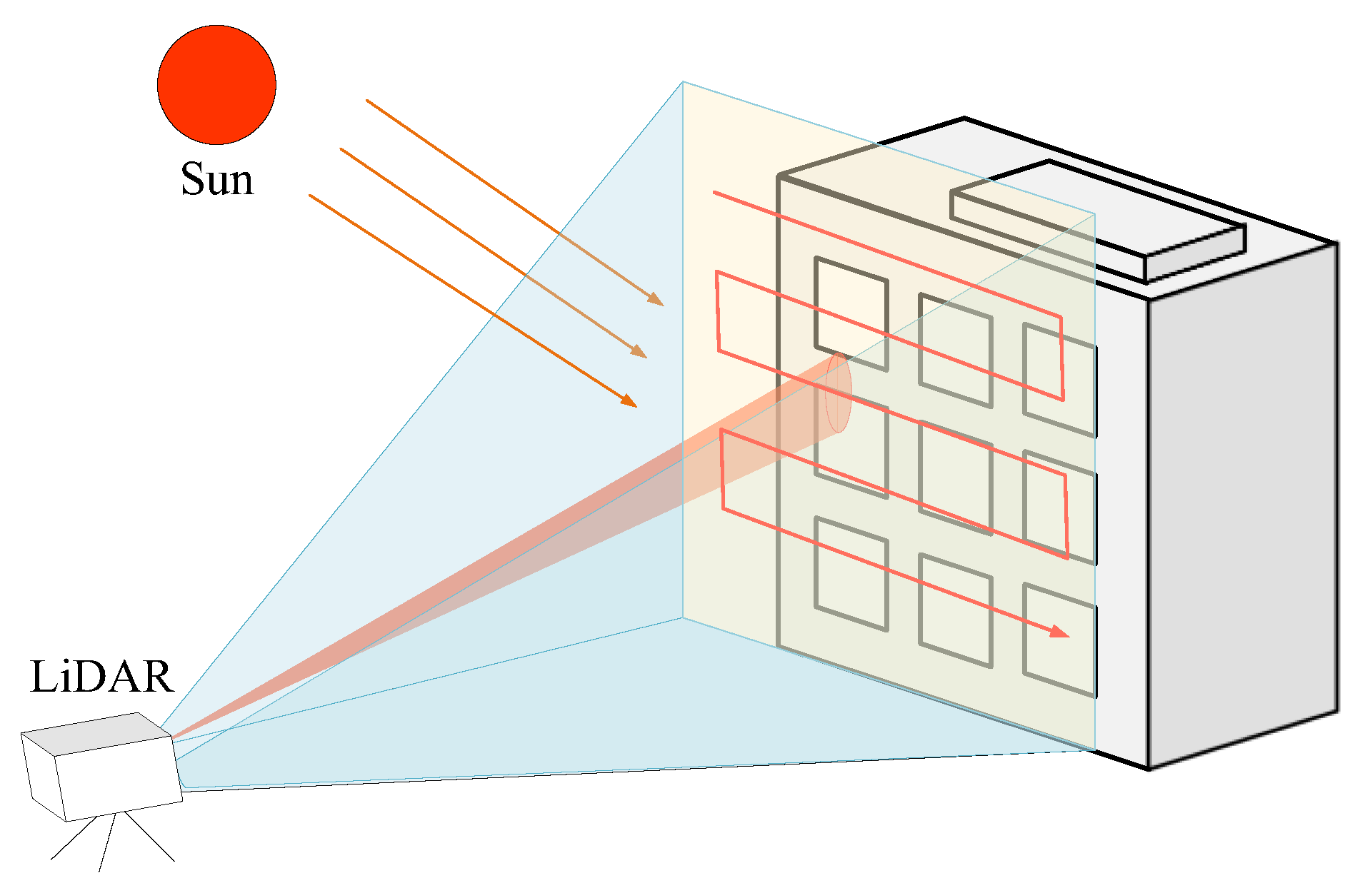
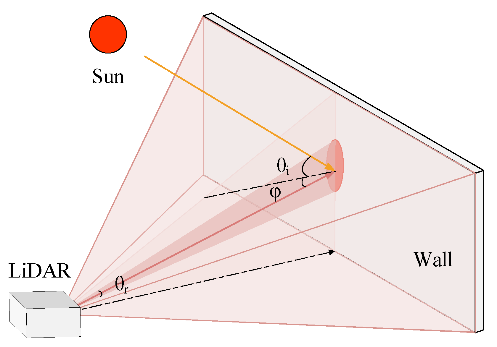
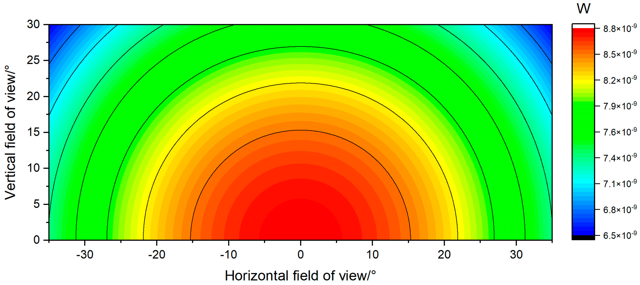
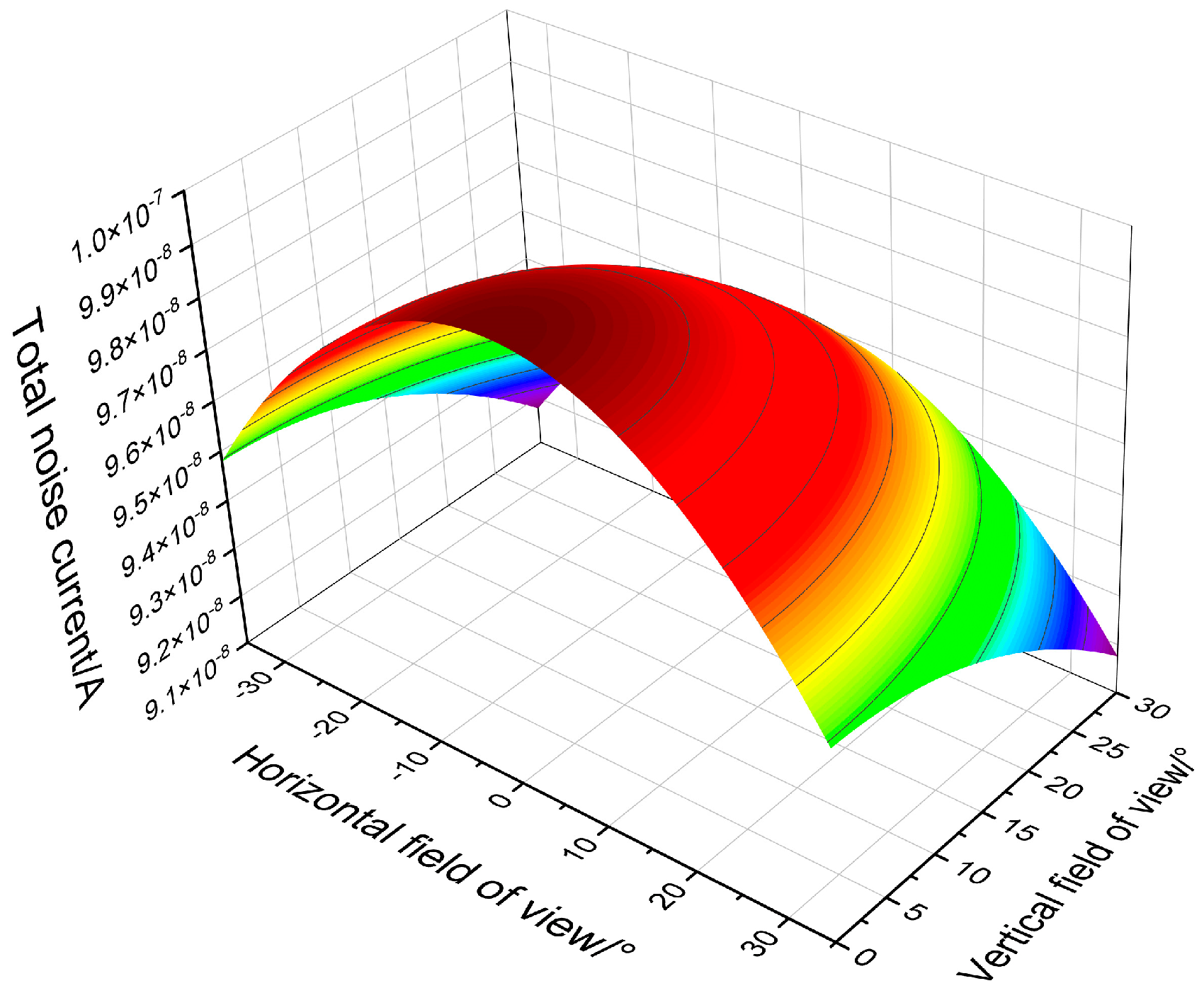
2. Influence of Background Noise

Noise in the LiDAR system is caused by the superposition of various noises, which can be divided into internal device noise and external noise according to the source of noise [24]. Background noise at the receiving end includes signals irradiated or reflected onto the detector from undesired radiation sources such as the sun and artificial light sources [25]. In daytime photoelectric detection, external background noise is usually far greater than the noise of the internal device of the system, the radiation source is mainly the sun, and the energy is concentrated in the visible and infrared spectrum [26]. According to ASTMG173 solar spectral data, within the spectral response range of LiDAR, the corresponding irradiance of direct sunlight is high [27]. Therefore, when LiDAR scanning works under strong sunlight, its instantaneous receiving field of view changes rapidly, and the background noise in different fields of view varies greatly.

As shown in Figure 1, sunlight enters the receiving end through target reflection and atmospheric scattering, and the background light power affects the detection of weak signals by LiDAR. Under uniform atmospheric conditions, the irradiance E_λ of sunlight on the ground can be obtained by integrating the spectrum of sunlight near the ground. Letting the sunlight be a beam of parallel light, the angle between the light and the target surface normal is θ_i, the atmospheric one-way transmission is T_r, the target reflection coefficient is ρ, the receiving field angle is θ_r and the angle between the receiving optical axis and the target surface normal is ϕ. Then, the background radiation power received by the detector is as follows [28]:

$$P_b=\frac{\pi }{16}{\eta }_r{\theta }_r^2{D}_r^2\Delta \lambda [T_r\rho E_{\lambda }\cos {\theta }_i\cos \varphi +\pi N_{\lambda }(1-T_r)]$$

(1)

where D_r is the receiving optical aperture, η_r is the optical transmission of the receiver, Δλ is the spectral bandwidth of the filter, and N_λ is the radiance brightness of the solar spectrum scattered by the atmosphere.

As shown in Figure 2, a simple building wall is used as an example to simulate Equation (1) to understand the variation in the background noise at each angle at the receiving end in the detection field of view. We can assume that the sunlight is incident on the wall of a building perpendicular to the ground normally at an angle of 60°, and the LiDAR is parallel to the opposite side. The horizontal field of view detected by the laser radar is ±35°, the vertical field of view is 30°, the optical transmittance is 0.8, the receiving field of view angle is 2 mrad, the receiving optical aperture is 50 mm and the filter bandwidth is 20 nm. The one-way transmittance of the atmosphere is 0.99, the reflection coefficient of the wall is 0.5 and the radiant illuminance of the sunlight on the ground is 1000 W/m²/μm. The simulated background noise variation of the building wall in the scanning field of view is shown in Figure 3.

For LiDAR with APD detector, all noises are independent of each other [24], and the value of the received total noise current i_n is:

$$i_n^2=i_{ns}^2+i_{nb}^2+i_{nd}^2+i_{nt}^2+i_{Na}^2$$

(2)

where i_ns is the signal light shot noise current, i_nb is the background optical shot noise current, i_nd is the dark current noise, i_nt is the thermal noise current and i_Na is the total equivalent input noise current of the amplifier. According to each noise formula [29], it can be obtained as the following:

$$i_n^2=2eB{M}^{2}F[R_o(P_s+P_b)+i_{db}]+2eB{i}_{ds}+\frac{4KTB}{R_L}+i_{Na}^2$$

(3)

where e denotes the elementary charge, B is the noise bandwidth, M is the APD multiplication factor, F is the APD excess noise factor, R_o is the APD unit multiplication factor response rate, P_s is the received signal power, i_db is the multiplied (bulk) of the dark current, i_ds is the un-multiplied (surface) of the dark current, K is the Boltzmann constant, T is the temperature and R_L is the equivalent load resistance. Based on the background radiation results in Figure 3, the noise changes in the receiver are analyzed through Formula (3), as shown in Figure 4. The simulation parameters are shown in Appendix A 

Table A1. Simulation parameters.

Category	Parameter	Symbol	Value
APD	Responsivity	Rp	30 A/W
	Bandwidth	B	150 MHz
	Gain	M	100
	Total Dark Current	Id	50 nA
	Excess noise factor	F	3.9
	Equivalent load resistance	RL	1 kΩ
Amplifier	Integrated input current noise (rms)	iNa	20 nA

, and the proportion of background radiation to total noise current is shown in Appendix A Figure A1.

The influence of background noise on LiDAR can be analyzed based on the SNR [30]. For the pulse detection, the SNR of the system is the ratio of the out current or voltage between the signal and the noise:

$$SNR=\frac{R_{o}M{P}_s}{\sqrt{2eB{M}^{2}F[R_o(P_s+P_b)+i_{db}]+2eB{i}_{ds}+\frac{4KTB}{R_L}+i_{Na}^2}}$$

(4)

From Equation (4), it can be seen that the increase in background radiation noise reduces the SNR, while other parameters are kept constant. The variation in the noise current makes the LiDAR more easily generate false alarms when the signal is detected over the threshold, which greatly affects the detection efficiency.

In the detection, the LiDAR will misidentify the noise as a signal due to the interference of background radiation and device noise, which can be expressed by false alarm probability. Random noise probability density functions such as background radiation noise, detector noise and circuit noise all obey Gaussian distribution [31], and the statistical characteristics of noise voltage u_n can be expressed by the Gaussian probability density function:

$$\rho (u_n)=\frac{1}{\sqrt{2\pi }{\sigma }_n}\exp (-\frac{u_n^2}{2{\sigma }_n^2})$$

(5)

where σ_n is the root mean square (RMS) of the noise voltage.

The FAR of LiDAR is the probability that the amplitude of system noise exceeds the signal detection threshold. The detection threshold voltage is set as V_T, and the RMS of noise voltage is $\overline{\mathrm{V}}$_n. By integrating Equation (5), the FAR P_f is:

$$P_{\mathrm{f}}={\displaystyle {\int }_{V_T}^{\infty }\rho (u_n)}d{u}_n={\displaystyle {\int }_{V_T}^{\infty }\frac{1}{\sqrt{2\pi }\overline{V_n}}\exp (-\frac{u_n^2}{2{\overline{V}}_n^2})}d{u}_n$$

(6)

Using the error function to simplify, it can be expressed as:

$$P_{\mathrm{f}}=\frac{1}{2}-\frac{1}{2}\mathrm{er}f(\frac{V_{Ts}-[R_{\mathrm{p}}(P_s+P_b)+I_d]G}{\sqrt{2}{\overline{V}}_n})=\frac{1}{2}-\frac{1}{2}erf(\frac{V_T}{\sqrt{2}{\overline{V}}_n})$$

(7)

where R_p is the responsiveness of APD, I_d is the dark current of APD, G is the amplification factor of the amplifier circuit, and the expression of the error function erf(x) is as follows:

$$erf(x)=\frac{2}{\sqrt{\pi }}{\displaystyle {\int }_0^x\exp (-t^2)}dt$$

(8)

Threshold noise ratio TNR is defined as

$$TNR=\frac{V_T}{{\overline{V}}_n}$$

(9)

Therefore, the threshold voltage or value of the noise voltage of the receiver circuit can be dynamically adjusted according to the false alarm detection in the receiver, so that the TNR remains unchanged, thus maintaining the FAR Pf stable during signal detection, and achieving the purpose of suppressing the variable background noise.

3. Adaptive Suppression Method of Background Noise

3.1. Structure and Implementation

There are two main methods of CFAR control in LiDAR: one is to adjust the reverse bias voltage of the APD to change its multiplication factor, so that the noise amplitude of the system remains stable; the other is to adjust the threshold voltage of the signal discrimination comparator. The first method often requires ms-level response time due to the bandwidth limitation of the low-pass filter network of the high-voltage power supply, and the single detection time of the LiDAR is mostly us-level during real-time scanning, so the adjustment is generally based on the average background noise of the whole scanning field of view, which cannot meet the demand of fast adjustment of the background noise change in the single detection. Compared with the first method, the signal detection threshold network has a larger bandwidth, and the response speed can reach ns-level. Therefore, the false alarm caused by fast variable background noise can be effectively solved by adaptive adjustment of the signal detection threshold.

The implementation structure of the adaptive method is shown in Figure 5, which is mainly composed of a noise quantization unit, threshold adjustment unit and signal processing unit. The noise quantization unit is used to detect and quantify the received noise rapidly. According to the detection noise in the receiver, the threshold adjustment unit adjusts the signal identification threshold voltage V_Ts and noise identification threshold voltage V_Tn through the cascaded voltage network. In addition to completing the traditional APD bias control, the signal processing unit also receives the output of the noise detection unit during single pulse detection and controls the DAC to correct the signal threshold voltage according to the noise quantization value.

The implementation of the adaptive method can be divided into two stages. During the LiDAR operation, it can be divided into two periods, before the time of light emission T₁ and after the time T₂, according to the working state of the laser, as shown in Figure 6. At the beginning of each detection, the system generates a pulse laser emission command. After receiving the pump signal of the excitation source, the laser needs a period of time T₁ to make the working material in the optical resonator achieve complete particle number reversal and then output the laser. At this time, the detection-varied background noise is not affected by the laser, and the system-ranging measurement window is closed, which is helpful to quantize background noise and adjust the threshold of signal identification. Therefore, the adjustment circuit compares and quantifies the noise quickly through the noise quantization unit during the time T₁ and controls the cascade network to complete the rapid adjustment of the signal threshold voltage. In a single detection, the power of background noise will continue to float for the moving target. Therefore, when the threshold voltage is rapidly adjusted by the cascade network, the noise quantization unit will continue to work during the detection time T₂, and the quantized result will be recorded in the signal processing unit as the correction value. The DAC is controlled by the signal processing unit to change the reference voltage V_ref of the cascade network, which simultaneously realizes the correction of the signal detection threshold voltage V_Ts and noise detection threshold voltage V_Tn.

3.2. Critical Modules Implementation

3.2.1. Noise Detection

Rapid and accurate noise detection and quantization is a prerequisite for realizing adaptive threshold regulation. There are two common noise detection methods. One is the integral quantization of noise voltage, which has the disadvantage of low speed and is easily affected by capacitance leakage current and temperature coefficient [32]. The other is to quantify the noise by counting the pulse times of the noise discrimination threshold. This method has the advantages of simple circuit implementation and fast detection speed. Due to the non-ideal factors of the devices in the actual system, the noise pulses drift and overlap. For the noise detection in a short time, there is a deviation in quantifying the noise only by the counting output pulses of the comparator. Therefore, the noise detection method is optimized in this paper.

False alarm probability can also be expressed by false alarm time [33]. False alarm probability P_f is the ratio of the time τ_sum when the envelope actually exceeds the threshold and the total time T_sum that can exceed the threshold:

$$P_{\mathrm{f}}=\frac{{\tau }_{sum}}{T_{sum}}=\frac{\frac{1}{N}{\displaystyle \sum _{k=1}^N{\tau }_k}}{\frac{1}{N}{\displaystyle \sum _{k=1}^N{T}_k}}=\frac{{\displaystyle \sum _{k=1}^N{\tau }_k}}{{\displaystyle \sum _{k=1}^N{T}_k}}$$

(10)

where τ_k is the duration of pulses exceeding the threshold, and T_k is the interval time between adjacent noise pulses exceeding the threshold. Therefore, the threshold voltage of signal discrimination can be adjusted by measuring the changes in τ_sum. For the noise pulse exceeding the threshold, the pulse duration is obtained by measuring the pulse width.

The discrimination comparator used is a continuous-type comparator, which cannot quantify the pulse width directly. Therefore, a dynamic comparator is designed for threshold detection of noise in this paper. While detecting the noise, the duration of the detected noise pulse can be obtained. The basic structure of the dynamic comparator designed is shown in Figure 7.

M1–M5 constitute the pre-amplifier circuit, M6–M14 constitute the latched comparator, and M12 is the reset tube. When the clock CLK is at low level, M12 is turned on to make the voltages at O and P equal, so as to avoid the unequal residual charges at O and P, thus affecting the accuracy of the comparator. The SR latch circuit is composed of two NOR gates which are cross-connected at both ends.

The noise detection threshold voltage of the noise comparator needs to be set in a reasonable range. According to Formula (10), since the receiver noise should be detected and quantified in time T₁ and fed back to the cascade network to completed the threshold control before laser pulse output, the total time T_sum can be approximated as T₁, and the probability of false alarm is P_f1. Thus, the total time t_s1 of actually exceeding the noise threshold can be obtained:

$$t_{s1}=P_{\mathrm{f}}{T}_{sum}=P_{\mathrm{f}1}{T}_1=T_1[\frac{1}{2}-\frac{1}{2}\mathrm{e}\mathrm{r}f(\frac{V_{Tn}}{\sqrt{2}{\overline{V}}_n})]$$

(11)

where V_Tn is the noise detection threshold. Therefore, the relationship between the corresponding V_T and the $\overline{\mathrm{V}}$_n in time T₁ can be obtained.

$$V_{TN}=\sqrt{2}{\overline{V}}_{n}er{f}^{-1}(1-\frac{2t_{s1}}{T_1})$$

(12)

The laser emission pulse period time is T_L, and the false alarm probability in time T₂ is P_f2; then, the proportional relationship between noise detection time T₁ and T₂ is the following:

$$\Delta n=\frac{t_{s1}}{t_{s2}}=\frac{P_{\mathrm{f}1}{T}_1}{P_{\mathrm{f}2}{T}_2}=\frac{P_{\mathrm{f}1}{T}_1}{P_{\mathrm{f}2}(T_L-T_1)}$$

(13)

From Formula (13), it can be known that under the same FAR, when the detection period is large and the noise detection time is short, namely T₂ >> T₁, the pulse duration t_s1 will be very small. Due to the limitation of the bandwidth of the detection system, t_s1 may not be detected, so t_s1 needs to satisfy the following:

$$t_{s1}>t_{set}\approx 2t_r\approx \frac{0.7}{B}$$

(14)

where t_set is the settle time, t_r is the pulse rising edge time, and B is the system bandwidth. Substituting this into Formula (12), the relationship between noise detection threshold V_Tn, time T₁ and system bandwidth B can be obtained.

$$V_{Tn}<\sqrt{2}{\overline{V}}_{n}er{f}^{-1}(1-\frac{1.4}{T_{1}B})$$

(15)

Since the time of noise detection is very short, the pulse width of random noise in the large-bandwidth receiver is quite small, so the dynamic comparator needs to operate at a high clock frequency in order to compare and quantify the noise as much as possible in the limited noise detection time. With dynamic comparators, the quantization resolution of the over-threshold noise duration is equivalent to the quantization number N_ck of the comparator during the noise detection time, which depends on the clock cycle T_ck of the comparator:

$$N_{ck}=\frac{T_1}{T_{ck}}=T_1{f}_{ck}$$

(16)

where f_ck is the clock frequency of the comparator, provided by the signal processing unit. The quantization of noise pulse width can be based on Nyquist’s theorem, and the clock frequency is generally more than 5 times the bandwidth of the detection system in practical application.

3.2.2. Threshold Adjustment

The adjustment of the signal threshold is self-adaptive through a cascaded network of current-type architecture and DAC output voltage, as shown in Figure 8. The adaptive process is divided into two steps. Firstly, the current source network is controlled to rapidly adjust the signal threshold voltage according to the quantization value of noise detection in time T₁. Secondly, the noise quantization unit continues to work in time T₂. The quantization result is taken as the correction value. After this detection, the DAC is controlled by the signal processing unit to adjust the reference voltage V_ref of the current source network to achieve the correction of the threshold voltage V_Ts and V_Tn.

Since the signal threshold regulation time is very short in ns-level, the design uses current steering architecture to achieve fast change in the signal threshold. It controls the current source through the switch for stacking output and can directly drive the resistive load without the buffer circuit of the resistance voltage divider network, thus avoiding the establishment time of the buffer circuit and providing high-speed regulation. The correction function of DAC is realized by changing the input bias voltage of the current source array. The reference voltage provided by the DAC is first converted to reference current, and then converted by the bias circuit to the input bias voltage of the current source array. Therefore, through the interaction of the circuit, the correction function is realized.

The current source is a sleeve structure composed of CMOS with high output impedance. The current source is controlled by a switch and ideally its output current is

$$V_{Ts}=I_{out}{R}_T={\displaystyle \sum _{k=0}^{N-1}{b}_k{I}_{ref}{R}_T}$$

(17)

where I_out is the output current, R_T is the load impedance, k is the number of current sources connected to the load, and I_ref is the reference current. Additionally, the number of current sources determines the variation range of FAR during rapid adjustment. The reference current I_ref is controlled by V_ref of the DAC.

The adjustment of threshold value can be determined by the FAR and detection probability requirement of the system. Assuming that the detection threshold cannot exceed the maximum false alarm probability required by the system as P_Fmax, according to the FAR Formula (7), under no signal, the following can be obtained:

$$P_{\mathrm{Fmax}}\ge \frac{1}{2}-\frac{1}{2}\mathrm{e}\mathrm{r}f(\frac{V_{Ts}-(R_{\mathrm{p}}{P}_b+I_d)G}{\sqrt{2}{\overline{V}}_n})$$

(18)

$$V_{T\mathrm{s}}\ge \sqrt{2}{\overline{V}}_{n}er{f}^{-1}(1-2P_{F\max })+(R_{\mathrm{p}}{P}_b+I_d)G$$

(19)

The threshold voltage is related to the designed FAR of the system. According to the parameters in

Table 1. Solar height and illuminance data.

Time/a.m.	8	9	10	11	12
Solar altitude/°	13.3	22.6	30.2	35.3	37.1
Illuminance/lux	6387	12,960	22,120	27,010	32,550

, when the FAR is set at 0.1%, the simulation result is shown in Figure 9, and the optimal value of the detection threshold V_Ts should be taken at the intersection of the simulation result surface and the plane of the designed FAR.

4. Experimental Results

In order to verify the practical effect of the method, the experiments were carried out based on the self-developed LiDAR of team. The LiDAR is controlled by an external program so that it can work in conventional mode, fast mode, and adaptive mode, respectively. Among them, the traditional mode only adjusts the APD bias voltage. In addition to adjusting the bias voltage, the fast mode also quickly adjusts the detection threshold voltage through the current steering architecture, and the adaptive mode adds the DAC feedback correction method on a fast mode basis. The diagram of the experimental scene is shown in Figure 10. The LiDAR adopts the same laser repetition frequency and power to detect the same area using the above three modes, respectively, and then the acquired point cloud of the target area is compared and analyzed. The main parameters of the LiDAR used in the experiment are shown in Appendix B

Table A2. Main parameters of LiDAR system.

Category	Parameter	Symbol	Value
Laser	Wavelength	λ	1064 nm
	Repetition frequency	f	100 KHz
	Average transmitted laser power	Pt	1 W
	Beam divergence angle	θt	1 mrad
	Pulse width	tp	5 ns
APD	Responsivity	Rp	36 A/W
	Receiving aperture	Dr	30 mm
	Rise Time	tr	2 ns
	Gain	M	100
	Total Dark Current	Id	50 nA
	Filter bandwidth	∆λ	10 nm
Optics	Optical efficiency of the receiving system	ηr	0.7
	Optical efficiency of the transmitting system	ηt	0.95
	Receiving field angle	θr	2 mrad
	Horizontal scanning field angle	θH	70°
	Vertical scanning field angle	θV	30°

.

Although the comparison can be directly observed from the LIDAR point cloud acquired using different methods, this comparison is rough, because the noise accumulates over time in the experiment, and each scanning does not take exactly the same amount of time. In order to quantify and analyze the experimental data, this paper refers to the evaluation method in [34] and introduces the parameter noise ratio P_m, which is used as an objective measure of the background noise suppression effect by calculating the ratio of noise to itself in the point cloud. The definition of the noise ratio P_m is as follows:

$${\mathrm{P}}_m=\frac{N_{ns}}{N_{og}}=\frac{N_{og}-N_{de}}{N_{og}}$$

(20)

where N_og is the number of original point clouds, N_de is the number of denoised point clouds, and N_ns is the number of noise points.

The laser radar detection experiment was carried out on a clear night, and the point cloud was collected as the basic data, as shown in Figure 11a. The original point cloud is denoised by the point cloud denoising program in the MATLAB, and the result of point cloud data processing is shown in Figure 11b. Then, the original point cloud and the denoised point cloud data are subtracted to obtain the noise points:

$${\mathrm{P}}_m=\frac{N_{og}-N_{de}}{N_{og}}=\frac{1944944-1944879}{1944944}=3.34\times {10}^{-5}$$

(21)

According to Formula (21), the noise ratio of the LiDAR at night is about 0.003%.

LiDAR detection experiments were conducted multiple times during clear daylight hours. The illuminance values at that time were measured by UNI-T’s UT383 illuminance meter, while the local solar height at the corresponding time of the day was queried on the Internet, and the recorded data are shown in Table 1.

From 8:00 to 12:00, each time with an interval of one hour, the LIDAR was controlled to work in three modes for detection experiments, and the collected point cloud data at 8 a.m., 10 a.m. and 12 a.m. are shown in Figure 12. From the three-dimensional point cloud image, it can be seen that the noise in the traditional mode is the highest in the daytime, and it increases with the enhancement in background radiation. Compared with the traditional mode, the data of point cloud by using the fast mode has less noise, and the suppression effect is better than the former under strong background radiation. Compared with the above two modes, the noise of point cloud by using the adaptive mode is the lowest, and the noise suppression effect is the best under strong background radiation.

The noise of point cloud is analyzed according to Equation (20). From 8 o’clock to 12 o’clock, the comparison results of noise ratio under different methods in the experiment are shown in Figure 13b. The experimental results show that the noise ratio increases to more than 0.045% in the traditional mode, and rapidly increases to 0.08% when the background radiation is strong. The noise ratio measured in the fast mode is more than 0.028%, which is better than the traditional mode. The noise ratio of the adaptive mode is the lowest. Even at 12 a.m., the noise ratio is 0.012%, which proves that the adaptive method has a good ability to suppress background noise. Figure 13b shows the proportion of noise reduction of these two modes at different times compared with the traditional mode. It can be seen that the proportion of noise reduction of the adaptive mode is more than 80% compared with the traditional mode.

In this paper, the adaptive method achieves noise suppression by circuit adjustment at each detection. Compared with the back-end software noise reduction processing method, it has great advantages in real-time detection. For the LiDAR with the laser emission frequency of 100 kHz, each adjustment can be completed in a period of 10 us. Per reference [34], a comparison is shown in

Table 2. Comparison of suppression methods.

Name	Noise Reduction Percentage	Processing Time Per Point	Implementation Mode
Bunny radius filtering method	83.9%	238 us	software
Dragon radius filtering method	82.8%	261 us	software
Piecewise adaptive threshold method	96.5%	289 us	software
This work	80.1%	10 us	hardware

.

5. Conclusions

In order to effectively suppress the interference of the background radiation noise in the instantaneous detection field of view on the system, the influence of the background radiation noise and the detection performance of the system is analyzed. According to the principle of CFAR control, on the basis of the traditional adjustment method, an adaptive suppression method of LiDAR background noise is realized through the adaptive threshold adjustment current steering architecture with a back-end DAC correction. In order to solve the problem of accurate noise detection quantification in a short time, a dynamic comparator is used to replace the traditional continuous comparator, and the measurement of the pulse duration of the noise is added to improve the noise detection accuracy. Finally, the experiment is carried out based on the LiDAR designed by our team, and the experimental results show that under the strong background noise, compared with the data obtained by the traditional method, the noise ratio can be reduced by more than 80%, which has a better background noise suppression capability. However, this method increases the complexity and design difficulty of the hardware, and has certain application limitations. It is suitable for laser radar with non-mobile scanning applications. For mobile applications, the noise change is more complex, and the DAC correction algorithm needs to be further improved, which is also the direction of future research.

References

1. Alain, Q.; Olivier, M.; Xavier, S. Analytic Model for Optimizing a Long-range Pulsed LiDAR Scanner for Small Object Detection. Appl. Opt. 2019, 58, 5496. [Google Scholar]
2. Yang, B.; Tang, W.; Xu, S.Y. Real-time and High-precision Ranging Method for Large Dynamic Range of Imaging LiDAR. Infrared Laser Eng. 2020, 49, 118–123. [Google Scholar]
3. Guo, D.; Wang, C.; Qi, B. Application of DMLF in Pulse Ranging LiDAR System. Appl. Sci. 2021, 11, 1032. [Google Scholar] [CrossRef]
4. Song, Z.Q.; Zhu, J.G.; Xie, T.P. Research progress on security LiDAR. Laser Optoelectron. Progress. 2021, 58, 28–42. [Google Scholar]
5. Gomes, T.; Roriz, R.; Cunha, L.; Ganal, A.; Soares, N.; Araújo, T.; Monteiro, J. Evaluation and Testing System for Automotive LiDAR Sensors. Appl. Sci. 2022, 12, 13003. [Google Scholar] [CrossRef]
6. Wang, W.; Chang, X.; Yang, J.; Xu, G. LiDAR-Based Dense Pedestrian Detection and Tracking. Appl. Sci. 2022, 12, 1799. [Google Scholar] [CrossRef]
7. Candan, C.; Tiken, M.; Berberoglu, H.; Orhan, E.; Yeniay, A. An Experimental Study on Km-Range Long-Distance Measurement Using Silicon Photomultiplier Sensor with Low Peak Power Laser Pulse. Appl. Sci. 2021, 11, 403. [Google Scholar] [CrossRef]
8. Kurtti, S.; Baharmast, A.; Jansson, J.P. A Low-noise and Wide Dynamic Range 15MHz CMOS Receiver for Pulsed Time-of-Flight Laser Ranging. IEEE Sens. J. 2021, 21, 22944–22955. [Google Scholar] [CrossRef]
9. Ding, H.B.; Wang, Z.Z.; Liu, D. Comparison of De-noising Methods of LiDAR Signal. Acta Opt. Sin. 2021, 41, 9–18. [Google Scholar]
10. Zhou, X.; Sun, J.F.; Fan, Z.G.; Li, S.N.; Lu, W. Research on Detection Performance Improvement of Polarization GM-APD LiDAR with Adaptive Adjustment of Aperture Diameter and Spatial Correlation Method. Opt. Laser Technol. 2022, 155, 108400. [Google Scholar] [CrossRef]
11. Teo, T.A.; Wu, H.M. Analysis of Land Cover Classification Using Multi-Wavelength LiDAR System. Appl. Sci. 2017, 7, 663. [Google Scholar] [CrossRef] [Green Version]
12. Lin, S.L.; Wu, B.H. Application of Kalman Filter to Improve 3D LiDAR Signals of Autonomous Vehicles in Adverse Weather. Appl. Sci. 2021, 11, 3018. [Google Scholar] [CrossRef]
13. Fu, C.; Zheng, H.; Wang, G.; Zhou, Y.; Chen, H.; He, Y.; Liu, J.; Sun, J.; Xu, Z. Three-Dimensional Imaging via Time-Correlated Single-Photon Counting. Appl. Sci. 2020, 10, 1930. [Google Scholar] [CrossRef] [Green Version]
14. Pradeep, G.; Vignesh, R.; Sandeep, K. A strip line technique based 1 Gb/s, 70-dB linear dynamic range transimpedance amplifier towards LiDAR unmanned vehicle application. Microelectron. J. 2022, 126, 105477. [Google Scholar]
15. Zhang, Z.; Chen, P.; Mao, Z.; Pan, D. Polarization Properties of Reflection and Transmission for Oceanographic LiDAR Propagating through Rough Sea Surfaces. Appl. Sci. 2020, 10, 1030. [Google Scholar] [CrossRef] [Green Version]
16. Lv, H.; Wang, R. Application of Avalanche Photodiode Constant False Alarm Rate Control in Laser Imaging System. Infrared Laser Eng. 2002, 31, 44–47. [Google Scholar]
17. Carrara, L.; Fiergolski, A. An Optical Interference Suppression Scheme for TCSPC Flash LiDAR. Imagers. Appl. Sci. 2019, 9, 2206. [Google Scholar] [CrossRef] [Green Version]
18. Ravil, A.; Barry, G.; Fred, M.; Alexander, G.; Ahmed, S. Simple approach to predict APD/PMT lidar detector performance under sky background using dimensionless parametrization. Opt. Lasers Eng. 2006, 44, 779–796. [Google Scholar]
19. Nguyen, T.T.; Cheng, C.H.; Liu, D.G.; Le, M.H. Improvement of Accuracy and Precision of the LiDAR System Working in High Background Light Conditions. Electronics 2022, 11, 45. [Google Scholar] [CrossRef]
20. Huntington, A.S.; Williams, G.M.; Lee, A.O. Modeling False Alarm Rate and Related Characteristics of Laser Ranging and LiDAR Avalanche Photodiode Photoreceivers. Opt. Eng. 2018, 57, 1. [Google Scholar] [CrossRef]
21. Zhou, B.; Liu, H.X.; He, X. Effect of background radiation on APD multiplication factor under the compensation of constant false alarm Rate. Acta Photonica Sin. 2018, 47, 56–62. [Google Scholar]
22. Hou, Z.F.; Lang, J.H. Design of Receiving Circuit in Long-distance Laser Range Finding Based on Variable Background-adaptation. Electro-Opt. Tech Appl. 2018, 33, 36–40. [Google Scholar]
23. Ouyang, J.H.; Huang, G.H.; Chen, P.F. Study of Constant False Alarm Rate Controlling Technique based on FPGA in LiDAR. J. Infrared Millim. Waves 2009, 28, 50–53. [Google Scholar] [CrossRef]
24. Andre, B.; Stefan, H.; Roman, B. Analytical Evaluation of Signal-to-noise Ratios for Avalanche- and Single-photon Avalanche Diodes. Sensors 2021, 21, 2887. [Google Scholar]
25. Dai, Y.J. Lidar Technology; Publishing House of Electronics Industry (PHEI): Beijing, China, 2010; pp. 193–195. [Google Scholar]
26. Guo, W.R.; Li, P.; Chen, H.M. Interference from Scattered Sunlight on Photodetector Posed in Different Angles. J. Detect. Control 2009, 31, 41–45. [Google Scholar]
27. Lin, J.; Bu, X.Z.; Han, W. Design of Pulsed Laser Rangefinder Under Background Light Noise. Foreign Electron Meas. Techno. 2017, 36, 117–120. [Google Scholar]
28. Ma, H.B.; Luo, Y.; He, Y. The Short-Range, High-accuracy Compact Pulsed Laser Ranging System. Sensors 2022, 22, 2146. [Google Scholar] [CrossRef]
29. Huang, G.H.; Ouyang, J.H.; Shu, R. Influence of Background Radiant Power on the Signal-to-noise Ratio of Space-borne Laser Altimeter. J. Infrared Millim. Waves 2009, 28, 58–61. [Google Scholar] [CrossRef]
30. Bissonnette, L.R. Multiple-scattering LiDAR Equation. Appl. Opt. 1996, 35, 6449–6465. [Google Scholar] [CrossRef]
31. Dong, J.W. Suppression of Background Radiance of Airborne Laser Radar. Electron. Opt. Control 2009, 16, 84–87. [Google Scholar]
32. Lv, Y.G.; Sun, X.Q. Principles and Applications of Laser Antagonism; National Defense Industry Press: Beijing, China, 2015; pp. 212–214. [Google Scholar]
33. Skolnik, M.I. Introduction to Radar Systems, 3rd ed.; Publishing House of Electronics Industry: Beijing, China, 2007; pp. 29–33. [Google Scholar]
34. Ren, B.; Cui, J.Y.; Li, G. A Three-dimensional Point Cloud Denoising Method Based on Adaptive Threshold. Acta Photonica Sin. 2022, 51, 0212003. [Google Scholar]
Figure 1. Effect of background radiation on LiDAR.
Applsci 13 03772 g001
Figure 2. Diagram of background radiation simulation.
Applsci 13 03772 g002
Figure 3. Simulation results of background radiation.
Applsci 13 03772 g003
Figure 4. Variation in total noise current.
Applsci 13 03772 g004
Figure 5. Adaptive suppression background noise implementation structure.
Applsci 13 03772 g005
Figure 6. Diagram of adaptive adjustment time.
Applsci 13 03772 g006
Figure 7. Schematic of dynamic comparator circuit.
Applsci 13 03772 g007
Figure 8. Threshold adjustment cascade architecture.
Applsci 13 03772 g008
Figure 9. Relationship between detection threshold and FAR.
Applsci 13 03772 g009
Figure 10. Diagram of LiDAR experiment scene.
Applsci 13 03772 g010
Figure 11. LiDAR point cloud of night (a) original data and (b) denoised data.
Applsci 13 03772 g011
Figure 12. Comparison of three modes of LIDAR point cloud. (a) Point cloud obtained by traditional mode at 8 a.m. (b) Point cloud obtained by fast mode at 8 a.m. (c) Point cloud obtained by adaptive mode at 8 a.m. (d) Point cloud obtained by traditional mode at 10 a.m. (e) Point cloud obtained by fast mode at 10 a.m. (f) Point cloud obtained by adaptive mode at 10 a.m. (g) Point cloud obtained by traditional mode at 12 a.m. (h) Point cloud obtained by fast mode at 12 a.m. (i) Point cloud obtained by adaptive mode at 12 a.m.
Applsci 13 03772 g012aApplsci 13 03772 g012b
Figure 13. Comparison of experimental results. (a) Noise ratio measured by three methods at different times. (b) The percentage of noise reduction at different times for the two methods compared with the traditional method.
Applsci 13 03772 g013