Abstract
Broadcasting, radar, sonar and space telecommunication systems use phased arrays to produce directed signals to be transmitted at the desired angle. This system requires a large number of antenna elements. The presence of faulty element(s) in an array causes asymmetry, which results in a deformed radiation pattern with higher sidelobe levels. Higher sidelobe levels indicate waste of energy by transmitting and receiving signals in unwanted directions. Hence, it is important to develop a method that detects faulty elements and corrects the radiation pattern. To correct the failed radiation pattern, failed elements in an array must be identified first. There have been various studies conducted on linear array failed radiation pattern correction and the finding of faulty elements, but investigation on the planar array is limited. Further, the optimization suggested for linear arrays does not necessarily work for the planar array. In this study, planar array faulty antenna detection was developed with pattern search (PS), simulated annealing (SA), and particle swarm optimization (PSO) methods by reducing the Signal to Noise Ratio (SNR) as the objective function. The analysis was varied for 8 × 8 and 6 × 6 planar arrays with different types of failures. The results were compared to find the best method to identify the faulty element’s location in a planar array. The pattern search method produced outstanding results in finding the faulty element’s locations by providing 100% accuracy for all types of failure, while other methods failed to do the same.
1. Introduction
The usage of a phased array antenna is a well-known method for generating signals to be directed at a chosen angle. The wide usage of phased array antennas in space systems is undeniable [1]. The introduction of 5G telecommunication and Massive-Input-Massive-Output (MIMO) created a necessity for a huge number of antennas to be present in a planar array at transmitter and receiver ends. An increased number of antennas increases the failure probability in an antenna system. Antenna failure(s) in an array affects the symmetrical structure, which will severely damage the radiation pattern and cause the sidelobe levels to be increased, weakening the null depth and null shift [1].
The normal method is to obtain near-field measurements at the antenna to identify the faulty element in an array [2,3,4,5]. However, in systems that are unreachable to humans, such as spacecraft, this conventional method is impractical [6]. Another technique to identify faulty elements is by using test couplers and calibration probes. These methods are difficult to operate and also expensive [7]. This demands extra investigation into a far-field radiation patterns to locate the array’s defective element(s) [8].
On the other hand, publications [9,10,11,12] have proposed methods that can be used to correct the failed radiation pattern. However, to make the adjustments to the array, information on the location of the failed element is required.
There is much research on linear array faulty element detection. The methods include the bacteria foraging [13], neural network [14,15], fast Fourier transform [16], firefly algorithm [17] and compressed sensing methods [18,19]. For a huge number of elements in an array, Khan S. U. et al. recommend a parallel coordinate descent, implemented using a hybrid genetic algorithm [19] and a hybrid cultural algorithm with differential evolution [20]. The methods that work for linear arrays do not necessarily work for a planar array.
For planar array, in [21], Chen Y.S. and Tsai I. worked on a systematic process of detection of failed components in arrays with cumulative sum (CUSUM) and radiation pattern correction, with least square estimation for both linear and planar arrays. They used hardware results for the detection and correction process. For planar arrays, they worked on 8 × 8 array sizes with 30% element failures. In [22], V. Puri and S. Puri used particle swarm optimization in a space-borne planar array with a 2 × 2 array size and one faulty element. Kusunose. K. and Arai. H. in [23] discussed detecting faulty elements in a planar array with cross-scanning along the x and y axis in 2D scanning. Ref. [24] uses a three-layer MLP neural network to train a network using failed radiation with the back-propagation learning mode. This work considers the mutual coupling effects from the failed element, with the simulated failed radiation pattern of a 6 x 6 array.
This paper extends the search for a suitable optimization method using metaheuristic algorithms such as the Particle Swarm Optimization (PSO), Simulated Annealing (SA), and Pattern Search (PS) methods for faulty element detection for antennas in a planar array in the MATLAB environment. In this study, a failed radiation pattern is generated for a planar array with some failed antennas. Then, the optimization methods discussed above were developed to identify the faulty element location in the planar array. The results of the methods are discussed, and finally, a successful method is recommended to identify faulty elements in the planar array.
2. Methodology
The methodology consists of developing an 8 × 8 element planar array, modelling and optimizing the developed model with four different optimization methods. This paper investigates a suitable optimization method to find failed elements in a planar array using failed radiation patterns, where the optimization is done in MATLAB through simulation. The simulations were conducted with a 64-bit operating system, Intel(R) Core (TM) i7-4790 CPU processor, and 16 GB installed memory. This work has computer capability and software limitations. This optimization simulation is for research purposes only. In real time, this procedure will be fast, because the procedure can be implemented with a Digital Signal Processor (DSP) with a parallel processing method. The suitable optimization method found in this study can be programmed with C language for DSP.
Planar array modelling involves generating failed radiation patterns for a planar array with a set of random failed locations. Then, SNR is calculated for the failed radiation pattern to evaluate the gain performance. Later, the optimization algorithm will try to detect the same failed location from the planar array modelling part. To find the initial failed locations, the optimization algorithm will assign new random failed locations, generate the new failed radiation pattern from the failed location, and find the respective SNR. The error value is found by determining the difference between the new failed radiation pattern’s SNR value and the initial radiation pattern’s SNR value. Ideally, the error value of the correct failed location will be zero. The error value is then minimized by the optimization method selected (SA, PSO, and PS) until the correct failed location is found. The design methodology is summarized in Figure 1.
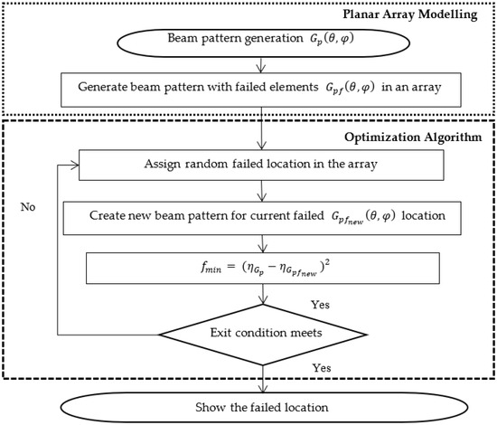
Figure 1.
Flowchart of faulty location detection methodology.
3. Problem Formulation
3.1. Planar Array Radiation Pattern Generation
The radiation pattern is generated by spatial signal processing, which uses phase shift and time delay to broadcast and receive sound waves according to the intended direction. The advantages of the phase shift, also known as the beam forming method, are less interference, high gain, improved device capability over omnidirectional signals, and focused directivity, resulting in improved signal quality.
This work adopted a phased array beamforming method from [25] for beam pattern generation with elements, an ultrasonic frequency of and a speed of sound in air at of the inter-element distance d avoiding grating is calculated from and .
With identical amplitudes of , the array factor beam pattern was normalized. The superposition of two-beam patterns, in the x-axis and in the y-axis, results in the planar array beam pattern . The planar array pattern’s beamforming output is given in (1).
where
and
where θ and φ = −90:1:90 are the scanning angle in x and y dimensions; γ is the directed angle; are the weights on each element; d is the distance between array elements; are array elements; and is the index.
Figure 2a represents a planar array with elements and a uniform distance between the elements; Figure 2b shows the corresponding element position or location in an planar array. Figure 3 shows the radiation pattern of an 8 × 8 planar array without any faulty elements.
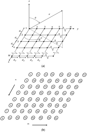
Figure 2.
(a) Planar array with M × N elements and uniform distance between the elements. (b) 8 × 8 planar array with corresponding positions of the elements.
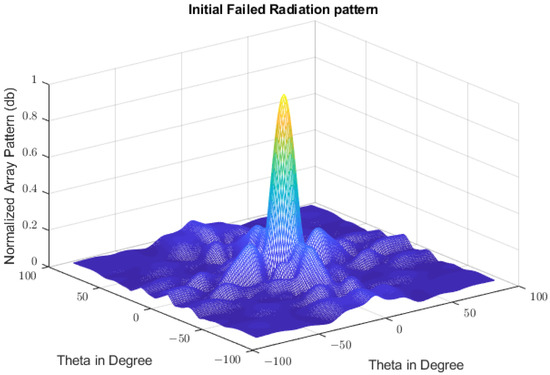
Figure 3.
Initial Radiation Pattern for 8 × 8 planar array without any faulty elements.
3.2. Failed Radiation Pattern Generation
To model failed beam patterns, failure array weights, and were utilised. In and , failed element weights were set to zero instead of one in and . The failed radiation pattern formulation is specified in (6) [26].
3.3. Types of Failure
The failed radiation pattern formula (6) is used for different types of failures, such as random type failure, row type failure, column type failure and group type failure, for 8 × 8 and 6 × 6 array configurations in the planar array. For the 8 × 8 planar array, 16 elements are failed, and for 6 × 6, 12 elements are failed. The number of failed elements for both array sizes is kept between 20% and 33.33% of the total number of elements, as correcting a huge number of elements will make the antenna system weak
For the random type of failure in an 8 × 8 array, 16 locations, i.e., [1, 3, 12, 17, 20, 26, 27, 35, 41, 46, 48, 50, 52, 53, 55, 60] are failed (non-functional), as shown in Figure 4; the faulty elements in the figure are unshaded, and the functional elements are shaded in black.
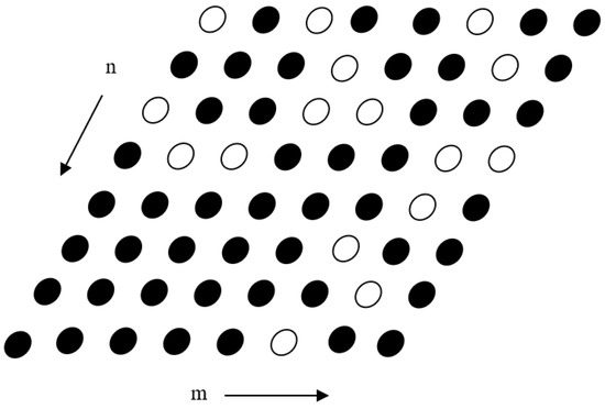
Figure 4.
Random type failure for 8 × 8 planar array.
Next, for the row type of failures, 2 rows of an 8 × 8 planar array are failed. For this purpose, all the elements in row 2 and row 5 are failed, which adds up to 16 elements. In Figure 5 below, the row type of failure for the 8 × 8 planar array is shown.
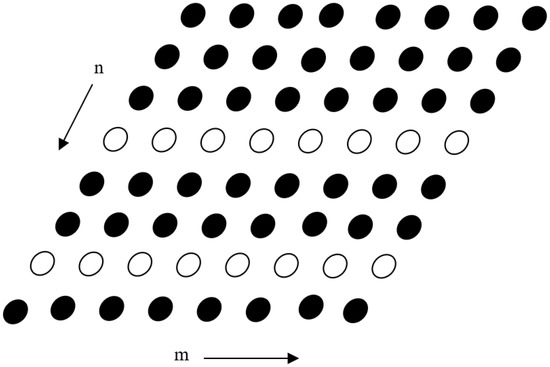
Figure 5.
Row type failure for 8 × 8 planar array.
For the column type of failures, 2 columns and 16 elements in an 8 × 8 planar array are failed. Here, all the elements in columns 2 and column 5 are failed. Figure 6 shows the column type of failure for the 8 × 8 planar array.
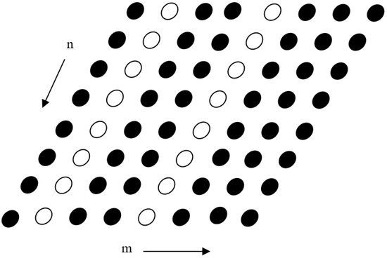
Figure 6.
Column type of failure for 8 × 8 planar array.
For the group type of failures, 16 elements in a form of 4 groups with 4 elements (2 × 2) are failed. Figure 7 represents the group type of failure in the 8 × 8 planar array.
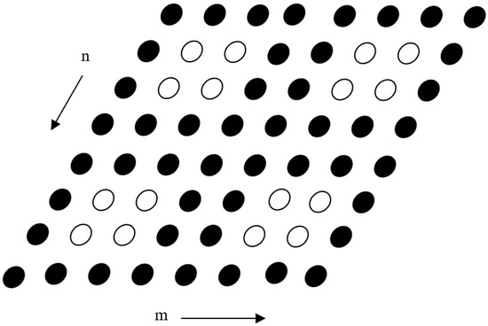
Figure 7.
Group type of failure for 8 × 8 planar array.
For the 6 × 6 planar array, similar types of failure were used but with 12 failed elements in total for each type of failure. The types of failure are listed in Table 1.

Table 1.
The 8 × 8 and 6 × 6 planar array failure types.
3.4. Performance Measure of the Radiation Patterns
SNR, is used to assess the gain performance of the failed radiation patterns. The SNR is the ratio of the main beam above −3 db, , and to the sidelobes of each radiation pattern, as specified in (7).
4. Optimization Algorithms
Currently, metaheuristic algorithms are applied in various fields, such as engineering, economics, politics, and management [26]. A balance between growth and divergence is essential to tackle day-to-day hitches in the fields efficiently [27]. Many nonlinear optimization issues can be solved by selected optimization techniques for a specific type of problem [28]. In this study, an optimization algorithm was developed to identify failure location(s) in a planar array.
After obtaining failed radiation patterns and SNR values for initial random failed locations, the optimization algorithm was developed. The optimization algorithm was programmed in such a way that the optimization starts by failing a new set of random failed locations. Then, the failed radiation pattern for the newly failed random location, , is calculated by Equation (8), and SNR for , is calculated with Equation (9).
The objective function is minimized by the optimization methods with SNR of both the initial failed radiation pattern, and newly failed radiation pattern,, with random failed locations. The optimization will reduce at each iteration with new sets of random locations until the lowest is found. When there is no difference between and the correct failed location is identified. is defined in Equation (8).
The search method and minimization criteria vary for each type of optimization method and are explained in the next section.
4.1. Pattern Search Optimization
The pattern search optimization method uses a set of pattern vectors to choose points to search at each iteration [29]. At each step, the algorithm looks for a set of points, known as a mesh, that enhances the objective function. At each step, the algorithm polls the points in the current mesh to determine the values of their objective functions. The algorithm will terminate polling when it discovers a point with an objective function lower than the current point. This is referred to as a successful poll, and the next iteration will use it as the current point. A poll is considered unsuccessful if the algorithm is unable to identify a point that enhances the objective function. For the unsuccessful poll, the current point remains unchanged in the following poll. After a successful poll, the mesh size, is multiplied by 2, and if the poll is unsuccessful the is reduced by 0.5.
Then, the vector is added to the point with the best objective function value obtained previously. The optimization stops and returns the optimal failed location once it meets the termination conditions.
An advantage of PS is it has a characteristic of global convergence, where it searches throughout the search range, which means it does not remain at a local minimum. PS can be easily implemented in mathematics and optimizations because it is developed with simple mathematic operations. PS consists of an array defined as a matrix to perform a restricted search [30]. The matrix is defined as mesh, and the current mesh is reduced by a set of survey constraints, which reduces the objective function [31]. The set of survey constraints ensures algorithm convergence. Figure 8 shows the pattern search optimization algorithm in a flowchart representation [32].
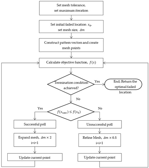
Figure 8.
Flowchart of the pattern search optimization algorithm.
4.2. Simulated Annealing Optimization
Simulated annealing is often used to solve unconstrained and bound-constrained optimization problems. The SA method uses the process of heating a solid and then gradually reducing the temperature to reduce defects. This consequently minimizes the system energy.
In SA, a new set of points is produced randomly at each iteration. The new point is defined by the probability distribution of the current temperature scale. If the new point lowers the objective function, the algorithm accepts a new point as the current point. The algorithm also accepts some worse points, which raises the objective function with an acceptance function described in Equation (9) [33]. This is to avoid the optimization being trapped in local minima instead of moving to global minima.
where Δ = new objective − old objective; T = temperature.
As the iteration goes on, this method uses an annealing schedule that systematically reduces the temperature [34]. The search of the algorithm converges to a minimum as the temperature reduces. In the end, the optimal solution is found. Figure 9 describes the simulated annealing optimization algorithm in a flowchart representation [35].
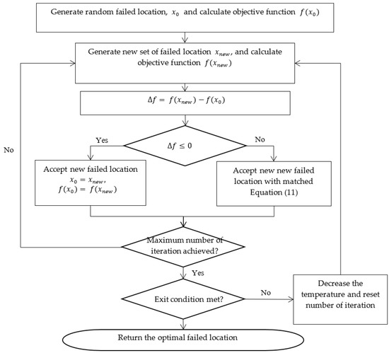
Figure 9.
Flowchart of the simulated annealing optimization algorithm.
4.3. Particle Swarm Optimization
PSO is a population-based algorithm developed using description by Kennedy and Eberhart [29], with some modifications suggested by Montes and Coello Coello [36] and Pedersen [37]. This method is inspired by bird flock swarming [29]. Particles in the algorithm attack the best solution found or found by any member of the swarm. The population then can merge around one location, determine a few locations, or continue to move.
The PSO algorithm starts with generating initial particles with initial velocities that move in steps at a specified area. The algorithm assesses each particle’s objective function at each step. The algorithm defines each of the particle’s new velocities following this assessment. The algorithm re-evaluates after the particles move. The lowest value is identified as the best function site after the objective function is assessed at each particle position. The best location for the particle, its best locations of the particle neighbours, and current velocity are taken into account when choosing new particle velocities. The method iteratively updates the best location, neighbouring particles, positions, and velocities. The algorithm iterates until it reaches the stopping condition. The steps of the algorithm are listed in the flowchart in Figure 10 [38].
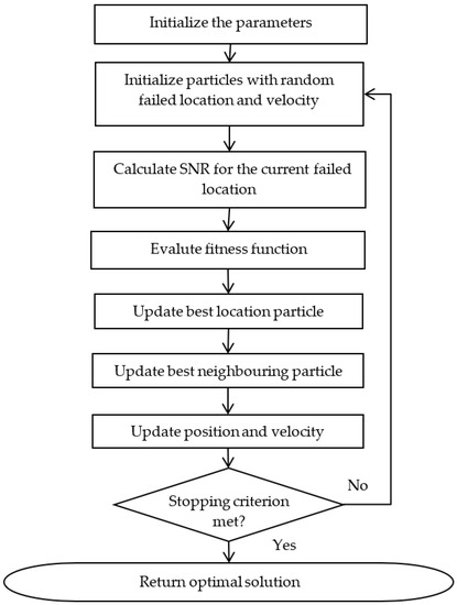
Figure 10.
Flowchart of Particle Swarm Optimization algorithm.
The results of each optimization method are discussed in the next section. At the end of the paper, an optimization method that detects the correct failure location for a planar array is proposed.
5. Results and Discussion
5.1. Modelling Results
Planar arrays with 8 × 8 and 6 × 6 array sizes were chosen to be modelled, with an interelement distance of λ/2. Failed radiation patterns were generated using Equation (6). It is assumed that all active elements are weighted as ones and all failed elements as zeros. For the 8 × 8 array, 16 elements were failed, and for the 6 × 6 array, 12 elements were failed.
A failed radiation pattern of an 8 × 8 planar array with a set of random locations, i.e., [1, 3, 12, 17, 20, 26, 27, 35, 41, 46, 48, 50, 52, 53, 55, 60] was assigned with zero weights. All the other active elements were weighted as ones. Figure 11a shows the Initial Failed Radiation Pattern of the 8 × 8 planar array with random failed locations, and Figure 11b shows the respective weight distribution.
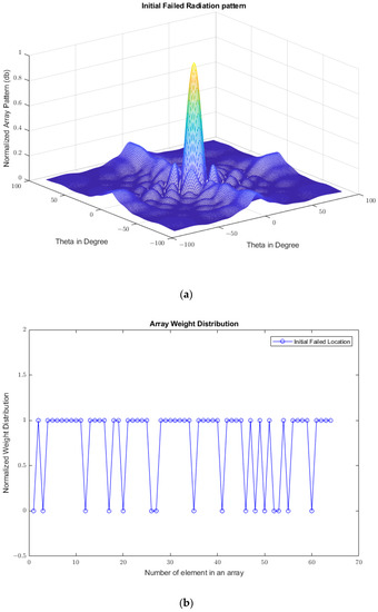
Figure 11.
(a) Initial Failed Radiation Pattern. (b) The weight distribution of Initial Failed Radiation Pattern.
5.2. Optimization Results
The initial Failed Radiation Pattern is then compared with the new failed radiation pattern, with the failed location optimized by optimization methods elaborated earlier. The optimization flow shown in Figure 1 is followed to obtain the results. The results show that the optimization algorithm developed managed to identify the failed locations in a planar array.
The pattern search method is successful in detecting all 16 failed locations in the 8 × 8 array for all types of failure. Figure 12, Figure 13, Figure 14 and Figure 15 show the results of failed location detection via the pattern search method for the random type, row type, column type and group type of failures, respectively, with 100% accuracy.
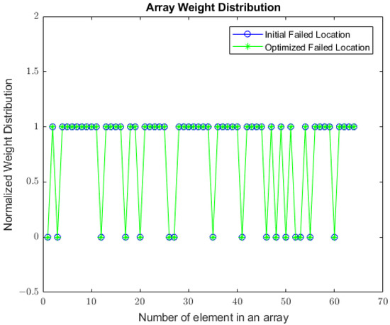
Figure 12.
Random failed locations found by pattern search method for 8 × 8 planar array.
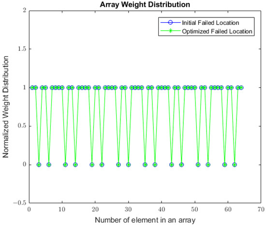
Figure 13.
Row type of failed location found by pattern search method for 8 × 8 planar array.
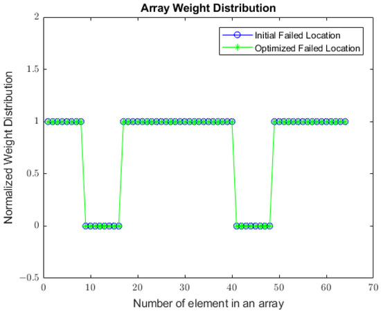
Figure 14.
Colum type of failed location found by pattern search method for 8 × 8 planar array.
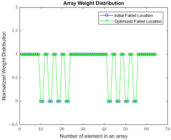
Figure 15.
Group type of failed location found by pattern search method for 8 × 8 planar array.
Next, the simulated annealing algorithm in 8 × 8 planar array detected 6 locations correctly out of 16 failed elements, giving 37.50% accuracy for random and row type failures; 5 correct detections in column type of failure with 12.50% accuracy; and only 2 correct location detections with 25% accuracy in the group type of failure.
Similarly, the PSO algorithm for the 8 × 8 planar array detected seven failed locations correctly in the random type of failure, which represents 43.75% accuracy. For the row type of failure, this algorithm failed to give any correct detection. For the column type of failure, this algorithm detected four locations correctly, which gives 25% accuracy. Lastly, for the group type of failure, this algorithm detected three locations correctly, which results in 18.75% accuracy.
The same optimization algorithms and the type of failure described above were developed for the 6 × 6 planar array. The results from using pattern search, simulated annealing, and particle swarm optimization methods for the 8 × 8 array size and 6 × 6 array size in planar arrays are listed in Table 2. The time taken for each of the optimization methods to identify the failed location is recorded for all types of failure in Table 2 below.
Table 2.
Results of Optimization Algorithm.
It is observed that the pattern search method provides better accuracy percentages for all types of failure in both 8 × 8 and 6 × 6 planar arrays. It managed to provide 100% accuracy for all types of failure for both array sizes. This method provides the best accuracy percentages compared to other methods for all types of failure. The success of this method of finding failure locations is due to the restricted search method, which operates in a mesh form, representing a matrix to find the global convergence. The current mesh is reduced by a set of survey conditions, which will lead to convergence to find a global minimum in long run.
The SA method in general provides 12.5% to 37.5% accuracy for all types of failure in an 8 × 8 array size in a planar array. For the 6 × 6 array size, the accuracy ranges from 8.33% to 62.5% for all types of failure.
On the other hand, the PSO method showed an accuracy range of between 6.25% and 31.25% for all types of failure in an 8 × 8 array-sized planar array. While in the 6 × 6 array, the range is from 12.5% to 58.33%.
The algorithms were written for the optimization methods to minimize the SNR as the objective function by varying the failed locations. SNR is calculated by the failed radiation pattern, because in real-time the only available data will be the failed radiation pattern. In addition, this work considered failed locations as completely failed elements. In the literature, for linear arrays, some methods are successful in finding 50% or 75% failure of faulty elements [19,39]. Moving forward, we can work on including detection failure elements that are not completely failed.
PSO and SA methods have tried to minimize the SNR, but the optimized failed locations given by the methods are not accurate. The percentage accuracy is given by the optimized location versus the initial failed location comparison. For each type of failure, optimization algorithms were run five times. Table 2 below summarizes the results.
6. Conclusions
An investigation was carried out for several types of failure, such as random, row, column, and group. Array sizes varied between 6 × 6 and 8 × 8 arrays. A suitable method to identify faulty element location was analyzed for PS, SA, and PSO methods. The pattern search method was successful in giving 100% accuracy in finding all types of failures compared to other optimization methods in both array sizes.
It is recommended that the PS method is used for all types of failure because the method detects the faulty elements in both 6 × 6 and 8 × 8 planar arrays accurately. Even though this method takes a relatively longer duration to converge compared to other methods, it detects failed elements in a planar array accurately. For the occurrence of faulty elements in far-field radiation patterns, the PS method can be applied in DSP to identify the failed locations in the planar array.
Since the PS method gives good results, this method can be incorporated with other optimization methods to form a hybrid optimization method to investigate failed element detection in a planar array and correction of the failed radiation pattern in a planar array. This work can also be extended to include parameters of MIMO or 5G communication applications. The external interference and internal noise effects can also be studied in simulation for robust analysis. However, in real-time applications, digital filters can be used to remove the noise. In the future, we can work on detecting elements that are not completely failed.
Author Contributions
Conceptualization, N.B., A.K.R., and F.N.; methodology, N.B., A.K.R., and F.N.; software, N.B. and F.N.; validation, N.B., F.N., and A.K.R.; formal analysis, N.B.; investigation, N.B.; resources, A.K.R.; data curation, N.B.; writing—original draft preparation, N.B.; writing—review and editing, N.B., A.K.R., and F.N.; visualization, N.B.,and A.K.R.; supervision, A.K.R., and F.N.; project administration, A.K.R.; funding acquisition, A.K.R. All authors have read and agreed to the published version of the manuscript.
Funding
This research was funded by UNITEN BOLD, grant number J510050002/2021064. The APC was funded by Universiti Tenaga Nasional (UNITEN) BOLD Publication Fund.
Institutional Review Board Statement
Not applicable.
Informed Consent Statement
Not applicable.
Data Availability Statement
Not applicable.
Conflicts of Interest
The authors declare no conflict of interest. The funders had no role in the design of the study; in the collection, analyses, or interpretation of data; in the writing of the manuscript, or in the decision to publish the results.
References
- Rao, S.; Acharya, O.P.; Patnaik, A. Antenna Array Failure Correction [Antenna Applications Corner]. IEEE Antennas Propag. Mag. 2017, 59, 106–115. [Google Scholar]
- Xiong, C.; Xiao, G.; Hou, Y.; Hameed, M. A Compressed Sensing-Based Element Failure Diagnosis Method for Phased Array Antenna During Beam Steering. IEEE Antennas Wirel. Propag. Lett. 2019, 18, 1756–1760. [Google Scholar] [CrossRef]
- Migliore, M.D.; Panariello, G. A comparison of interferometric methods applied to array diagnosis fromnear-fielddata. IEE Proc. Microw. Antennas Propag. 2001, 148, 261–267. [Google Scholar] [CrossRef]
- Lee, J.; Ferren, E.; Woollen, D.; Lee, K. Near-field probe used as a diagnostic tool to locate defective elements in an array antenna. IEEE Trans. Antennas Propag. 1988, 36, 884–889. [Google Scholar] [CrossRef]
- Bregains, J.C.; Ares, F.; Moreno, E. Matrix pseudo-inversion technique for diagnostics of planar arrays. Electron. Lett. 2005, 41, 19–20. [Google Scholar] [CrossRef]
- Lord, J.; Cook, G.; Anderson, A. Reconstruction of the Excitation of Array Antennas from the Measured Near-Field Intensity using Phase Retrieval. In Proceedings of the 1992 22nd European Microwave Conference, Helsinki, Finland, 5–9 September 1992; Volume 1, pp. 525–530. [Google Scholar] [CrossRef]
- Bucci, O.; Capozzoli, A.; D’Elia, G. Diagnosis of array faults from far-field amplitude-only data. IEEE Trans. Antennas Propag. 2000, 48, 647–652. [Google Scholar] [CrossRef]
- Choudhury, B.; Jha, R.M. Fault Detectionin Antenna Arrays. In Soft Computing in Electromagnetics Methods and Applications; Cambridge University Press: Cambridge, UK, 2016; pp. 124–154. [Google Scholar] [CrossRef]
- Patidar, H.; Mahanti, G.K. Failure correction of linear antenna array by changing length and spacing of failed elements. Prog. Electromagn. Res. M 2017, 61, 75–84. [Google Scholar] [CrossRef]
- Khan, S.U.; Rahim, M.K.A.; Aminu-Baba, M.; Murad, N.A. Correction of failure in linear antenna arrays with greedy sparseness constrained optimization technique. PLoS ONE 2017, 12, e0189240. [Google Scholar] [CrossRef] [PubMed]
- Yeo, B.-K.; Lu, Y. Array failure correction with a genetic algorithm. IEEE Trans. Antennas Propag. 1999, 47, 823–828. [Google Scholar] [CrossRef]
- Keizer, W.P.M.N. Element Failure Correction for a Large Monopulse Phased Array Antenna With Active Amplitude Weighting. IEEE Trans. Antennas Propag. 2007, 55, 2211–2218. [Google Scholar] [CrossRef]
- Acharya, O.P.; Patnaik, A.; Choudhury, B. Fault finding in antenna arrays using bacteria foraging optimization technique. In Proceedings of the 2011 National Conference on Communications (NCC), Bangalore, India, 28–30 January 2011; pp. 1–5. [Google Scholar] [CrossRef]
- Patnaik, A.; Christodoulou, C. Finding failed element positions in linear antenna arrays using neural networks. In Proceedings of the 2006 IEEE Antennas and Propagation Society International Symposium, Albuquerque, NM, USA, 9–14 July 2006; pp. 1675–1678. [Google Scholar] [CrossRef]
- Patnaik, A.; Choudhury, B.; Pradhan, P.; Mishra, R.K.; Christodoulou, C. An ANN Application for Fault Finding in Antenna Arrays. IEEE Trans. Antennas Propag. 2007, 55, 775–777. [Google Scholar] [CrossRef]
- Yadav, K.; Singh, H. Application of iterative fast Fourier transform for fault finding in linear array antenna with various fault percentage. In Proceedings of the 2014 Innovative Applications of Computational Intelligence on Power, Energy and Controls with their impact on Humanity (CIPECH), Ghaziabad, India, 28–29 November 2014; pp. 117–120. [Google Scholar] [CrossRef]
- Khan, S.U.; Qureshi, I.M.; Zaman, F.; Basit, A.; Khan, W. Application of firefly algorithm to fault finding in linear array santenna. World Appl. Sci. J. 2013, 26, 232–238. [Google Scholar] [CrossRef]
- Prajosh, K.P.; Khankhoje, U.K.; Ferranti, F. Fault diagnosis by a novel compressed sensing technique in a phased array with cosine squared element patterns. In Proceedings of the 2021 15th European Conference on Antennas and Propagation (EuCAP), Dusseldorf, Germany, 22–26 March 2021. [Google Scholar] [CrossRef]
- Khan, S.U.; Qureshi, I.M.; Naveed, A.; Shoaib, B.; Basit, A. Detection of Defective Sensors in Phased Array Using Compressed Sensing and Hybrid Genetic Algorithm. J. Sens. 2016, 2016, 6139802. [Google Scholar] [CrossRef]
- Khan, S.U.; Qureshi, I.M.; Zaman, F.; Khan, W. Detecting faulty sensors in an array using symmetrical structure and cultural algorithm hybridized with differential evolution. Front. Inf. Technol. Electron. Eng. 2017, 18, 235–245. [Google Scholar] [CrossRef]
- Chen, Y.-S.; Tsai, I.-L. Detection and Correction of Element Failures Using a Cumulative Sum Scheme for Active Phased Arrays. IEEE Access 2018, 6, 8797–8809. [Google Scholar] [CrossRef]
- Puri, V.; Puri, S. Detection of Defective Element in a Space Borne Planar Array with Far-Field Power Pattern Using Particle Swarm Optimization. J. Electron. Commun. Eng. 2015, 10, 17–22. [Google Scholar] [CrossRef]
- Kusunose, K.; Arai, H. Detection of Defective Element by Cross Scanning Near Field Examination for Symmetrical Planar Array. In Proceedings of the 2019 International Symposium on Antennas and Propagation (ISAP), Xi’an, China, 27–30 October 2019; pp. 5–6. [Google Scholar]
- Mallahza-deh, A.R.; Taherzadeh, M. Element Failure Diagnosis in a Planar Microstrip Array by the Use of Neural Networks. In Proceedings of the 2010 International Conference on Applications of Electromagnetism and Student Innovation Competition Awards (AEM2C), Taipei, Taiwan, 11–13 August 2010; pp. 294–298. [Google Scholar]
- Balanis, C.A. Antenna Theory, 4th ed.; John Wiley & Sons, Inc.: Hoboken, NJ, USA, 2016. [Google Scholar]
- Kumar, V.; Chhabra, J.K.; Kumar, D. Parameter adaptive harmony search algorithm for unimodal and multimodal optimization problems. J. Comput. Sci. 2014, 5, 144–155. [Google Scholar] [CrossRef]
- Katoch, S.; Chauhan, S.S.; Kumar, V. A review on genetic algorithm: Past, present, and future. Multimed. Tools Appl. 2021, 80, 8091–8126. [Google Scholar] [CrossRef]
- Lewis, R.M.; Torczon, V.; Trosset, M.W.; William, C. Direct Search Methods: Thenand Now Operated by Universities Space Research Association. J. Comput. Appl. Math. 2000, 124, 191–207. [Google Scholar] [CrossRef]
- Kenne-dy, J.; Eberhart, R. Particle Swarm Optimisation. In Proceedings of the ICNN’95-International Conference on Neural Networks, Perth, WA, Australia, 27 November–1 December 1995; Volume 4, pp. 1942–1948. [Google Scholar]
- Findler, N.V.; Lo, C.; Lo, R. Pattern search for optimization. Math. Comput. Simul. 1987, 29, 41–50. [Google Scholar] [CrossRef]
- Palacio-Morales, J.; Tobón, A.; Herrera, J. Optimization Based on Pattern Search Algorithm Applied to pH Non-Linear Control: Application to Alkalinization Process of Sugar Juice. Processes 2021, 9, 2283. [Google Scholar] [CrossRef]
- Zewail, I.; Saad, W.; Shokair, M.; El-dolil, S.A. Maximization of Total Throughput Using Pattern Search Algorithm in Underlay Cognitive Radio Network. Menoufia J. Electron. Eng. Res. 2017, 26, 307–319. [Google Scholar] [CrossRef]
- Ingber, L. Adaptive simulated annealing(ASA):Lessons learned. J. Control Cybern. 1996, 25, 33–54. [Google Scholar]
- Eglese, R. Simulated annealing: A tool for operational research. Eur. J. Oper. Res. 1990, 46, 271–281. [Google Scholar] [CrossRef]
- Zhou, A.-H.; Zhu, L.-P.; Hu, B.; Deng, S.; Song, Y.; Qiu, H.; Pan, S. Traveling-Salesman-Problem Algorithm Based on Simulated Annealing and Gene-Expression Programming. Information 2018, 10, 7. [Google Scholar] [CrossRef]
- Mezura-Montes, E.; Coello, C.A.C. Constraint-handling in nature-inspired numerical optimization: Past, present and future. Swarm Evol. Comput. 2011, 1, 173–194. [Google Scholar] [CrossRef]
- Pedersen, M.E. Good Parameters for Particle Swarm Optimization; Hvass Laboratories: Luxembourg, 2010. [Google Scholar]
- Youse-fi, M.; Omid, M.; Rafiee, S.; Ghaderi, S.F. Strategic planning for minimizing CO2 emission susing LP model based on forecasted energy demand by PSO Algorithm and ANN. Int. J. Energy Environ. 2013, 4, 1041–1052. [Google Scholar]
- Boopalan, N.; Ramasamy, A.K.; Nagi, F.H. Faulty antenna detection in a linear array using Simulated Annealing Optimization. Indones. J. Electr. Eng. Comput. Sci. 2020, 19, 1340–1347. [Google Scholar] [CrossRef]


Disclaimer/Publisher’s Note: The statements, opinions and data contained in all publications are solely those of the individual author(s) and contributor(s) and not of MDPI and/or the editor(s). MDPI and/or the editor(s) disclaim responsibility for any injury to people or property resulting from any ideas, methods, instructions or products referred to in the content. |
© 2023 by the authors. Licensee MDPI, Basel, Switzerland. This article is an open access article distributed under the terms and conditions of the Creative Commons Attribution (CC BY) license (https://creativecommons.org/licenses/by/4.0/).