Abstract
Frame analysis (FA) is known for its efficiency and low computer resource requirements. However, compared to finite element analysis (FEA), the applicability of FA for the seismic performance assessment of pile-supported wharves (PSWs) is limited, particularly in the ability to account for the kinematic force caused by ground displacement during an earthquake. This study aimed to develop a two-dimensional FA method for PSW seismic response analysis that considers a combination of inertial and kinematic forces. We performed FA and FEA and compared the results. First, we targeted the PSW model without considering the soil slope and discussed the spectral acceleration (SA) evaluation method for calculating inertial force. As a result, an equation for estimating a damping coefficient to evaluate the SA in accordance with the PSW width and natural period was proposed. Next, we targeted the PSW model by considering the soil slope and proposed a method to evaluate the kinematic force based on the amount of ground displacement and the soil spring characteristics. The results revealed that using the proposed method, FA, by considering kinematic and inertial forces, could reproduce the bending moments of the piles comparable to those calculated using FEA. Therefore, solely considering the inertial force for a PSW on a soil slope may cause the bending moment to be underestimated.
1. Introduction
Pile-supported wharf (PSW) is one of the main port facilities for transferring shiploads and ship berthing. PSWs installed in seismically active regions are prone to damage and loss of functionality due to earthquakes. The 1964 Niigata earthquake caused damage to PSWs due to lateral spreading [1] and the 1989 Loma Prieta earthquake caused the significant destruction of PSWs in the Port of Oakland, including pile head failure, settlement, and lateral spreading [2]. The 2010 Haiti earthquake affected the Port de Port-au-Prince when a PSW shifted toward the sea, sinking the gantry crane [3]. Such losses of PSW serviceability immediately affect the functions of entire ports, resulting in considerable economic losses. To mitigate the threat of seismic damage to a PSW, its seismic performance must be evaluated.
During earthquakes, the piles of PSWs are subjected not only to the inertial force transmitted from the wharf’s deck but also to the kinematic force caused by the ground displacement of the soil slope. The latter is usually more destructive because the lateral resistance of the pile is reduced during massive earthquakes [4]. In the case of piles embedded in a soil slope, a significant bending moment is generated by kinematic force [5]. Comparing the natural periods of PSWs with and without soil slopes, the former is shorter than the latter. Moreover, because the amplitude of the spectral acceleration (SA) is generally significant in the short period range, neglecting the soil slope in seismic design may result in dangerous outcomes, even if the kinematic force is negligible.
The seismic performance of PSWs can be precisely analyzed using soil-structure finite element analysis (FEA). Previous studies, such as by Boyke and Nagao [6], Nagao and Lu [7], and Lei Su et al. [8], have discussed the seismic responses of PSWs using this method.
In FEA, the structure and soil layer are modeled, and the complex problem is solved, such as the interaction between the structure and soil in the case of lateral spreading occurring by earthquakes. In design practice, however, FEA is not usually applied because it is time-consuming and requires advanced simulation programs.
On the contrary, frame analysis (FA) is a simpler method for analyzing the seismic response of the frame structure, such as PSW; therefore, SA is the standard method applied in design practice. However, SA has shortcomings including, e.g., the ground deformation due to earthquakes cannot be considered. The inertial force estimated from SA is applied to the PSW deck as a static load. The magnitude of SA is dependent on the damping coefficient and the value commonly employed by PSW engineering design is 0.03–0.05, with a typical PSW width of 20–60 m [9,10]. As for PSWs that exceed 100 m in width, the commonly estimated damping coefficient may not be appropriate. Consequently, establishing a method for predicting the damping coefficient of wide PSWs is necessary.
Several studies, such as by Tamura [11] and Smith et al. [12], have identified potential factors that may affect the damping of a structure, including material damping, structural connections, foundations, building height, and the hysteresis of yielding components. Iwashita and Hakuno [13] found that the larger the foundation depth, the greater the damping coefficient. Tamura [11] proposed methods to predict the damping coefficient as in Equations (1) and (2).
where H is the building height (m) and x is the deformation at the peak of the building (m). However, these equations were developed specifically for buildings. A simplified method for evaluating the optimum damping coefficient for the design practice of PSWs has not yet been proposed.
Several studies have addressed the impact of kinematic forces on pile design. The Japan Road Association (JRA) developed a widely used equation for predicting kinematic force [14]. The equation assumes a triangular-shaped distribution of soil pressure that depends on soil density, pile length, and diameter. The JRA code recommends that designers check for bending failure due to kinematic force and inertial force separately. Dobry et al. [15] conducted further research on kinematic force by undertaking six centrifuge model tests on single-pile foundations and suggested a soil pressure of 10.3 kPa on piles. He et al. [5] suggested that the soil pressure on piles was equivalent to the gross overburden pressure based on shaking table test results. Haigh and Madabhushi [16] measured a homogeneous soil pressure of 16 kPa on piles in a liquefiable stratum. Tang et al. [17] proposed a uniform pressure of 19.5 kPa based on data from a single-pile shaking table test.
Although existing lateral spreading soil pressure models have been proposed based on test results, significant differences have been observed among the soil pressures proposed by the studies described above. Therefore, selecting the correct kinematic force for pile design practice is challenging [18,19,20]. In addition, the suggested soil pressure models were obtained primarily from the results of single-pile tests. According to the FEA results of PSW pile groups on a gentle soil slope, the soil pressure decreases with increasing distance from the top of the slope [6]. Therefore, existing soil pressure models based on single-pile testing do not apply to pile group scenarios—a method of predicting the kinematic forces acting against pile groups on a soil slope needs to be developed.
In light of the lack of research on the effects of kinematic force and the damping coefficient on the seismic performance of a wide PSW on a gentle slope, this study aimed to develop a method to predict these variables. PSW seismic design using FA often neglects the effect of kinematic force on a gentle soil slope; generally, only inertial force has been considered. Furthermore, the change in the damping coefficient due to a change in PSW width has often been neglected in design practice, which could lead to overdesign.
The damping coefficient that should be used to calculate SA is assumed to vary depending on the PSW width. For this reason, we propose a method for setting the optimum damping coefficient for calculating SA according to the width of the PSW by creating cross sections of the PSW with various widths and by performing FEA. Furthermore, we propose a method for evaluating the kinematic force to be considered in FA using the FEA results.
2. Methods
2.1. Target PSW
The target PSW has a steel pipe pile foundation and a reinforced concrete deck. Fourteen PSW models with different widths were developed. To investigate the impact of soil slope displacement, we considered two scenarios for the FEA: one with a soil slope and one without a soil slope. The target PSW and ground configurations for Scenario 1 (without a soil slope) are depicted in Figure 1 and the configurations for Scenario 2 (with a soil slope) are depicted in Figure 2. The deck elevation is +4.00 m low water spring (LWS). The deck is supported by a group of steel pipe piles with diameters (Ø) of 1100 and 1200 mm that sit on seabed at −13 m LWS. The trestle bridge comprises a reinforced concrete deck and Ø1000 mm steel pipe piles. The wharf and trestle are connected and respond integrally to earthquakes.
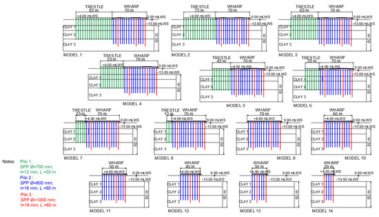
Figure 1.
Scenario 1 (without a soil slope) pile-supported wharf configurations.
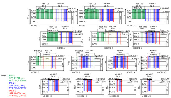
Figure 2.
Scenario 2 (with a soil slope) pile-supported wharf configurations.
The soil properties used in this study, which were obtained from previous research [6], are shown in Table 1. The soil consists of four silty clay layers, where Clay 0 at the ground surface is soft clay, and Clay 3 at the pile end is stiff clay. The shear wave velocity (Vs) for each soil layer was computed using the correlation equation given by Imai and Tonouchi [21] with the N-values from standard penetration tests (N-SPTs). The average shear wave velocity in the top 30 m (Vs30) at this site is 174.5 m/s, placing it in class E (soft ground), according to the Indonesian seismic code SNI 1726 2019 site classification [22].

Table 1.
Soil properties.
2.2. Finite Element and Frame Analysis Modeling
The PLAXIS 2D [23] program was used to create a 2D FEA model (Figure 3). PSW models were created with 15 node point triangular elements as plane strain models. This analysis used two consecutive loading phases: static loading (i.e., accounting solely for the PSW and soil self-weights) and seismic loading phases. In the static phase, the side boundary conditions were set as normally fixed, while the bottom boundary conditions were set as fully fixed. For the seismic loading phase, the side and bottom boundaries were set as free field and compliant base boundaries, respectively [24]. The seismic load was applied as a ground motion waveform at the base of the soil layer and in-plane seismic excitation was applied. To transmit ground motions in the frequency range of up to 10 Hz, the fine mesh option was chosen for mesh coarseness with a maximum mesh height of 2 m.
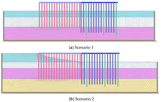
Figure 3.
Typical FEA model of the PSW.
In the FEA, the wharf deck was modeled using plate elements and the piles were represented using an embedded beam row element. The embedded beam row element enables the 2D modeling of piles with out-of-plane spacing, which has been validated by comparisons with a three-dimensional (3D) FEA simulation and data from actual testing. In the embedded beam row element, the pile is separated from the 2D soil model, which makes the soil mesh continuous. Special interface elements between the soil mesh and embedded pile are employed to consider the soil–pile interaction. Sluis et al. [25] compared the 2D embedded beam row model with the 3D embedded pile model for axial and lateral loading, and it was found that the displacement of an embedded beam row model was comparable to the 3D pile displacements. Dao [26] also demonstrated the applicability of the embedded beam row model by comparing the response of the embedded beam row model and experimental results.
The hardening soil small strain (HSS) model was implemented to account for the nonlinearity of soil. The HSS model is a variation of the hardening soil model that considers the increased stiffness of soils at small strains [24], which is described by two additional material parameters: the small strain shear modulus (G0 ref) and the shear strain level at which the small strain shear modulus decreases to 70% of its initial value (γ0.7).
To discuss the structural seismic response, various ground motions should be considered [27,28,29,30,31] together with site-specific ground motions [32,33]. The simulations used two waveforms with different characteristics: the 1968 Tokachi-Oki earthquake (TE) and the 2020 Mentawai earthquake (ME). The ME waveform was modified to match the target Indonesian site class SA [34]. These waveforms were deconvoluted at the bedrock, and the peak acceleration and duration were 0.210 g and 19 s for the TE and 0.215 g and 130 s for the ME, as illustrated in Figure 4. The structure’s inelastic behavior may have catastrophic consequences [35,36]; thus, many vital structures (e.g., PSW) were designed to remain in an elastic state during earthquakes. We focused on the elastic response of the PSW; therefore, we multiplied the waveforms by 0.8 to reduce their amplitude so that the structural members in the analysis remained in an elastic state during the earthquake.
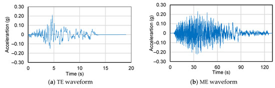
Figure 4.
Input waveforms.
The SAP 2000 [37] software was used to create a 2D FA model (Figure 5). Piles and beams were modeled as rigidly connected frame elements. To describe the relationship between the soil reaction (P) and the lateral displacement (Y) around the piles for each soil layer with depth, we used soil spring elastic-plastic P-Y curves. The P-Y curve for the spring properties was calculated using the L-PILE [38] computer program based on a study by Matlock [39]. Figure 6, Figure 7 and Figure 8 show the P-Y curves at different depths below the seabed. Figure 6 depicts the ultimate soil resistance for the Ø1000 mm pile at a depth of 1 m as 26.5 kN for Scenario 1 and 11.1 kN for Scenario 2. This difference is due to differences in the properties of the soil layers at the ground surface in Scenarios 1 and 2, where the undrained cohesion of the Scenario 1 surface layer (Clay 1) is greater than that of the Scenario 2 surface layer (Clay 0). The undrained cohesion was based on a correlation with N-SPT, according to Terzaghi et al. [40]. Figure 7 and Figure 8 describe the ultimate soil resistance for the Ø1100 and Ø1200 mm piles at a 1 m depth, which were 29 kN and 31 kN, respectively, for Scenarios 1 and 2. In general, the P-Y curve demonstrates that the larger the diameter of the pile, the greater the soil resistance.
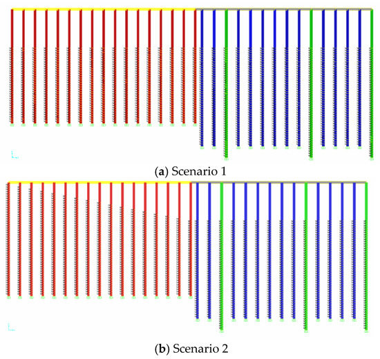
Figure 5.
Typical FA model of the PSW.
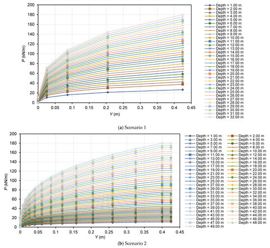
Figure 6.
P-Y curves for Pile 1 (Ø1000 mm).
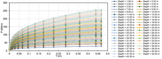
Figure 7.
P-Y curves for Pile 2 (Ø1100 mm).
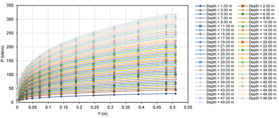
Figure 8.
P-Y curves for Pile 3 (Ø1200 mm).
2.3. Method for Calculating Inertial Force
Using the static equivalent approach, the inertial force of the PSW can be expressed as a multiplication of the total mass of the PSW above the seabed and the SA at the natural period of the PSW. For the FA, the inertial force was applied as a lateral force toward the seaward side at the top end of the PSW’s landward side.
To calculate the inertial force, the mass of the PSW was first calculated according to the various PSW widths. The elastic deflection was obtained by applying a small lateral load to the PSW and the PSW spring constant was determined by dividing the lateral load by the deflection. The natural period of the PSW was calculated by Equation (3).
where Tn is the PSW’s natural period, K is the PSW’s spring constant, and M is the PSW’s mass.
Next, we conducted a one-dimensional (1D) soil–column seismic response analysis to determine the ground surface waveform. A frequency domain analysis considering nonlinear soil characteristics was performed using DEEPSOIL software [41]. For the shear modulus and damping coefficient dependencies on the shear strain, we referred to Vucetic and Dobry [42] for cohesive soil. We then generated several SAs at the ground surface with varying damping coefficients to calculate the inertial forces. Using these inertial forces, we found the damping coefficient that offers the best fit between the FEA and FA acceleration.
2.4. Method for Calculating Kinematic Force
For the FA to account for slope displacement, the kinematic force was derived using the soil residual displacement distribution in front of the pile, taken from the FEA results. The kinematic force was determined based on the P-Y curves shown in Figure 6, Figure 7 and Figure 8. In conjunction with the residual displacement from the FEA, the soil reaction value in the P-Y curve was used as the kinematic force.
Our research also examined kinematic loading using the JRA method [14] for comparison. Regarding the single pile, the proposed JRA method shown in Equation (4) was used to measure the triangular-shaped distribution of soil pressure against the pile.
where Cs is the modification factor, which is set as 1 when the pile length is shorter than 50 m, 0.5 when the pile length is between 50 and 100 m, and 0 when the pile length is greater than 100 m. CL is the lateral pressure factor and is frequently set as 0.3, γL is the soft soil layer averaged unit weight (kN/m3), z is the pile depth below the ground surface (m), and D is the pile diameter (m).
3. Results and Discussion
3.1. Inertial Force
The PSW masses and natural periods calculated using Equation (3) are shown in Table 2. The largest PSW mass occurs in Model 1 due to its greatest width. Scenario 2 yields a smaller PSW mass and natural period than Scenario 1 because the pile length above the seabed is shorter in Scenario 2 due to the soil slope.
Table 2.
PSW masses and natural periods.
The SAs generated by the 1D soil–column seismic response analysis using TE and ME waveforms based on the damping coefficient (ξ) = 0.01–0.07 are illustrated in Figure 9 and Figure 10, respectively. Figure 9 shows that the TE waveform has a large SA in the period shorter than 1.0 s, with the largest SA being 1.0 g at 0.6 s. Figure 10 shows that the ME waveform has a large SA in a period longer than 1.0 s, with the largest SA being 1.9 g at 1.75 s.
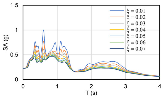
Figure 9.
Ground surface SA of the TE waveform.
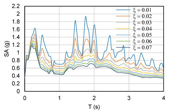
Figure 10.
Ground surface SA of the ME waveform.
The values of the inertial forces in Scenario 1 based on the TE and ME waveforms are shown in Table 3. The ME waveform produced a more significant inertial force than the TE waveform due to its larger SA for the PSW’s natural period.
Table 3.
Inertial forces for Scenario 1.
3.2. Kinematic Force
The FEA residual displacements of the TE and ME waveforms are described in Figure 11 and Figure 12, respectively. The displacement decreased with increasing distance from the top of the slope. The most significant displacement occurred at the top of the slope at 0.13 m and 0.25 m due to the TE and ME waveforms, respectively.
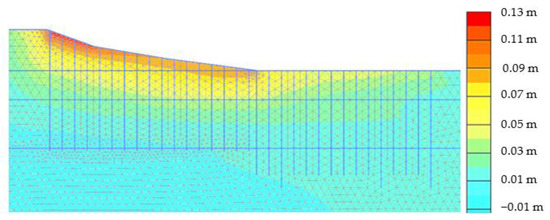
Figure 11.
FEA of the TE waveform: Residual displacement.
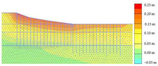
Figure 12.
FEA of the ME waveform: Residual displacement.
Figure 13 and Figure 14 depict examples of the kinematic force distribution calculated using the proposed method and the JRA method, respectively. The JRA method produces a more conservative smallest kinematic force (21 kN) than the proposed method (6.2 kN). The JRA method generates the same kinematic force at all distances from the top of the slope. In contrast, the proposed method demonstrates that the kinematic force is smaller at the toe of the slope than at the top of the slope because ground displacement is reduced with distance from the top of the slope. The kinematic force produced by the TE and ME waveforms differs. The ME waveform creates a larger kinematic force than the TE waveform due to its greater ground displacement (Figure 12). The JRA method does not account for waveform characteristics; it focuses only on soil unit weight and depth. Figure 14 depicts the triangular shape of the JRA kinematic force distribution and Figure 13 depicts the trapezoidal form of the proposed kinematic force distribution. The JRA method was computed based on the hypothesis that ground displacement occurs in the soft soil layer. Therefore, the kinematic force distribution is computed at the base of the Clay 2 soil layer. In comparison, the kinematic force distribution in the proposed method is based on the ground displacement determined by the FEA. Consequently, kinematic force is not estimated when there is no displacement in the soil layer.
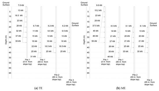
Figure 13.
Examples of kinematic forces using the proposed method.
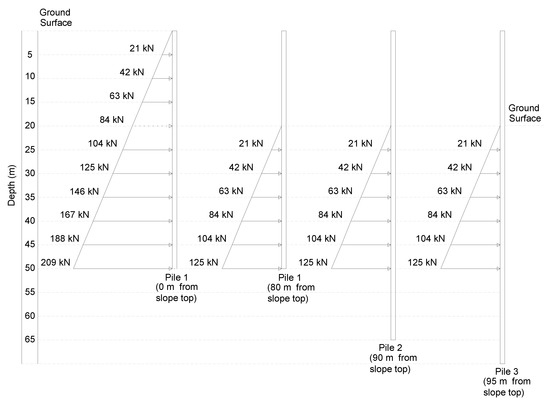
Figure 14.
Examples of kinematic forces using the JRA method.
3.3. Application of the Proposed Method
The SAs at the top left of the soil model for Scenario 1 for the various damping coefficients generated by the FEA are shown in Figure 15. The TE waveform has a large SA in the period shorter than 1.0 s and the ME waveform has a large SA in the period longer than 1.0 s.
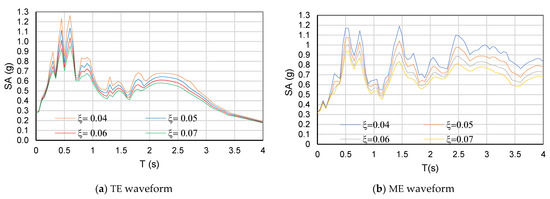
Figure 15.
FEA: Ground surface SAs with various damping coefficients.
The FEA results for Scenario 1 using the TE and ME waveforms are described in Table 4. The maximum PSW acceleration was obtained directly from the FEA results. The PSW’s natural period was derived from the predominant frequency of the Fourier spectra. The PSW maximum acceleration and Fourier spectra were generated for the top right (seaward side) end of the PSW deck. The PSW damping coefficients shown in Table 4 were determined so that the deck’s FEA maximum accelerations matched the SAs generated by the FEA ground surface motions, as shown in Figure 15.
Table 4.
FEA results for Scenario 1.
The PSW’s natural period in Scenario 1 was approximately 1.20 s. The deck’s maximum acceleration from the FEA results became larger as the width of the PSW became smaller. This is because structural rigidity decreases when the PSW becomes narrower, which increases PSW deformation and acceleration. The damping coefficient becomes smaller as the PSW width decreases. The largest value of the damping coefficient was 0.07 and the smallest value was 0.04.
Table 5 shows the FA results using the TE and ME waveforms. The largest deck’s maximum acceleration occurred in Model 14: 5.38 and 6.53 m/s2 for the TE and ME waveforms, respectively. In contrast, the smallest values occurred in Model 1: 3.61 and 5.29 m/s2 for the TE and ME, respectively.
Table 5.
FA results for Scenario 1.
The maximum acceleration for the PSW from the FA results at different damping coefficients was calculated using Equations (5) and (6):
where Dd is the PSW’s displacement, obtained from the FA; Td is the damped natural period; ξ is the PSW’s damping coefficient; and fn is the PSW’s natural frequency.
The following step was taken to determine the damping coefficients that produce the best fit between the deck’s maximum acceleration from the results of the FEA and FA. Table 5 describes the deck’s maximum accelerations from the FA that are closest to the FEA results; the damping coefficients that produce the closest values were set as the damping coefficients of the PSW.
A comparison of the FEA results (Table 4) with the FA results (Table 5) reveals good agreement between the two findings. Both analyses showed that the PSW’s natural period is around 1.20 s. The damping coefficient values in models 1–4, 5–9, 10–12, and 13–14 were 0.07, 0.06, 0.05, and 0.04, respectively. This result shows that even if the waveforms used in the analysis have different characteristics, the PSW still shows consistent damping coefficients. This is because the damping coefficients were mainly affected by the structural characteristics, such as the shape, construction material, and foundation.
We then conducted a parametric analysis to determine the variables influencing the PSW’s damping coefficient. The width, mass, natural period, and spring constant of the PSW were set as independent variables, and we employed a statistical analysis using multiple linear regression. To prevent the occurrence of highly correlated independent variables in the regression model, we conducted a multicollinearity test using the variance inflation factor (VIF) method.
The multicollinearity test demonstrated that the PSW width, mass, and spring constant have high VIF values of 1396, 6249, and 10,589, respectively. This result is understandable because as the PSW increases in width, the number of structural elements in the model also increases, causing the mass and spring constant to increase. Next, we removed the highly correlated variables (i.e., the mass and spring constants) to eliminate multicollinearity issues. Using multilinear regression analysis, we developed a damping coefficient prediction equation as follows:
where w is the PSW’s width (m) and Tn is the PSW’s natural period (s).
Equation (7) has a determination coefficient (R2) equal to 94% and a minimal standard error of 0.002, which indicates that the damping coefficient can be accurately predicted by Equation (7). The probability, or P-value, of the independent variable was less than the standard significance level of 0.05, indicating that the variable was statistically significant. Our study shows that the width of the PSW significantly affects the damping coefficient. Increasing the width of the PSW results in the incorporation of more structural elements (i.e., piles and beams) in the model, which could result in a more significant contribution of material damping to the structural damping, thereby increasing it.
To apply the proposed method to FA Scenario 2, we determined the damping coefficient using Equation (7). Then, using Figure 9 and Figure 10, we obtained the SA based on the PSW’s natural period from Table 2 and the damping coefficient from Equation (7). The SA obtained was multiplied by the PSW mass from Table 2 to produce the inertial force. The inertial forces in Scenario 2, based on the TE and ME waveforms, are shown in Table 6. The ME waveform generated a greater inertial force than the TE waveform due to its larger SA at the PSW’s natural period.
Table 6.
Inertial force for Scenario 2.
Figure 16 and Figure 17, respectively, depict the bending moment distributions due to the TE and ME waveforms for Scenario 2. The red line represents the result of the FEA, while the black and blue lines represent the results of the FA employing kinematic force determined by the proposed method (Figure 13) and the JRA method (Figure 14), respectively. The bending moment obtained from the FA using the proposed method agrees with the FEA results. In comparison, the FA bending moment produced by the kinematic force using the JRA equation yields more conservative results. For example, in Figure 16b, the FEA produced a maximum bending moment of 1222 kN·m, while the FA using the proposed method and the JRA method produced 1154 kN·m and 1559 kN·m, respectively.
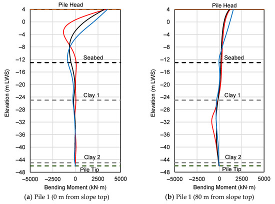
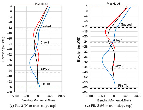
Figure 16.
Bending moment distribution of the PSW considering the inertial and kinematic forces due to the TE waveform (Scenario 2).
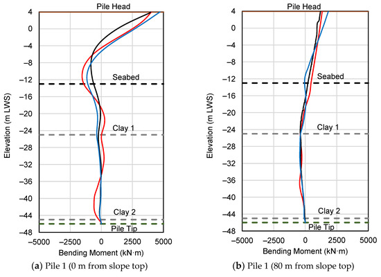
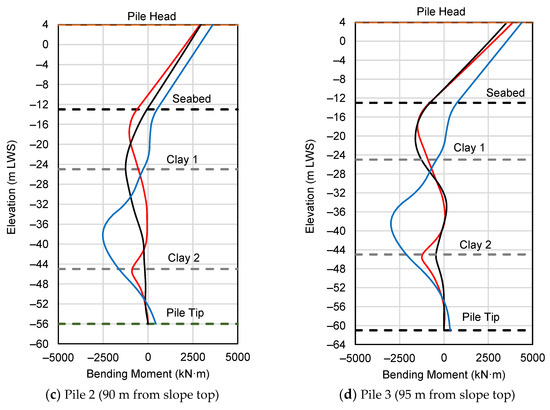
Figure 17.
Bending moment distribution of the PSW considering the inertial and kinematic forces due to the ME waveform (Scenario 2).
Figure 16c,d and Figure 17c,d show the differences in the bending moments observed at piles located outside the slope area. This indicates that at a depth of 36–40 m, the JRA method’s bending moment becomes excessive because of the triangular distribution of the kinematic force. By contrast, the bending moment calculated using the proposed method produced reasonable results compared to the FEA. For example, as shown in Figure 16c, at 40 m depth, the JRA method produced a bending moment of 1723 kN·m while the proposed method and the FEA produced bending moments of 166 kN·m and 115 kN·m, respectively.
It should be noted that the analyses shown in Figure 16 and Figure 17 were calculated considering both inertial and kinematic forces. Thus, although the JRA’s kinematic forces (Figure 14) used to produce Figure 16 and Figure 17 were identical, the outcome was not. This is because the inertial force was calculated using different ground surface waveforms (Table 6).
The FA’s bending moment distributions for Scenario 2 considered using only the inertial force (black line) and the FEA results (red line) due to the TE and ME waveforms, respectively, are compared in Figure 18 and Figure 19. The FA bending moment produced by the inertial force is only about half of the FEA bending moment. This indicates that the incorporation of kinematic force in the analysis is crucial for obtaining an appropriate bending moment in the case of a PSW on a soil slope.
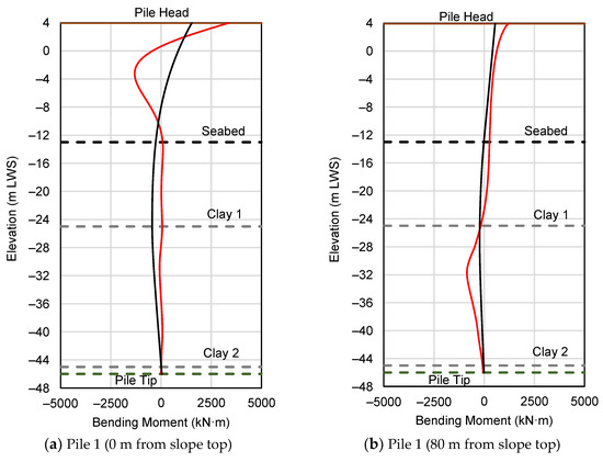
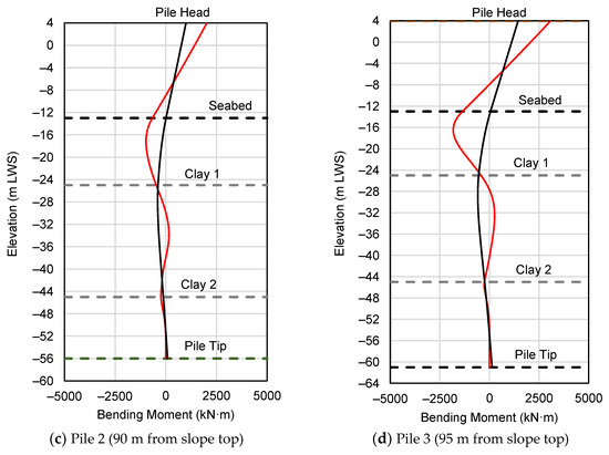
Figure 18.
Bending moment distribution of the PSW considering the inertial forces due to the TE waveform (Scenario 2).
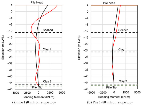
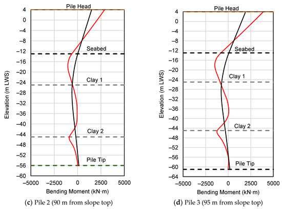
Figure 19.
Bending moment distribution of the PSW considering the inertial forces due to the ME waveform (Scenario 2).
The response of the piles subjected only to inertial force was comparable to that produced by either the response of the beam on the Winkler foundation or the response of the cantilever considering the free length of the pile (Figure 18 and Figure 19), where the primary factors are the flexural stiffness of the cantilever and pile’s free length (i.e., the sum of the characteristic length and protruding length of the pile). The bending moment caused by the kinematic force is mainly affected by the soil/pile stiffness ratio, the impedance contrast of the two soil layers, and the natural frequency of the soil stratum in relation to the input waveform [43,44]. At the boundary between soil layers, the bending moment considering the combination of the kinematic and inertial loads exhibits a relatively significant value (Figure 16 and Figure 17), showing that adding the kinematic load to the analysis could demonstrate the impact of the impedance contrast between the two soil layers.
4. Conclusions
To study the seismic performance of a wide PSW with a gentle soil slope, our research suggested an FA method that considers both inertial and kinematic forces based on the PSW damping coefficient. The main conclusions of this study are as follows:
- FA provides the fastest and most reliable calculation tools for assessing the seismic performance of PSWs and it is effective for considering the effect of kinematic forces. It is also able to produce bending moments that are comparable to those calculated using FEA.
- The typical damping coefficient employed in PSW seismic design is 0.05. Our research indicates that a wide PSW has a more significant damping coefficient than a typical smaller-width PSW. We provide an equation for calculating the PSW damping coefficient based on its width and natural periods.
- The bending moment of a PSW pile is generated by a combination of inertial and kinematic forces. The bending moment produced by the inertial force is only about half of the FEA bending moment. Adding kinematic force into the analysis could demonstrate the impact of soil displacement and the impedance contrast between the soil layers, thus producing a comparable result with FEA, considering only inertial forces for PSWs on a slope could lead to the underestimation of the bending moment. Even in the case of a PSW on a gentle slope, the effect of kinematic force is still significant.
- Seismic evaluations that consider only the inertial force or the kinematic force using the JRA equation are inappropriate, while seismic evaluations using the proposed method are highly applicable. The inability of the JRA method to estimate kinematic force was found in the bending moment distribution of the piles. At some depth, the bending moment became too large because of the triangular distribution of the kinematic force. The JRA method is unsuitable for calculating kinematic force caused by ground deformation because it produces a constant kinematic force regardless of the amount of ground deformation.
- The kinematic force in FA can be computed using ground displacement and soil spring characteristics. In conjunction with ground displacement (as determined by the FEA), soil reaction value can be used as a kinematic force with satisfactory results. A technique to estimate ground displacement without referring to FEA results will be developed in a future study.
Author Contributions
Conceptualization, C.B. and T.N.; methodology, C.B. and T.N.; software, C.B.; validation, C.B. and T.N.; formal analysis, C.B. and T.N.; investigation, C.B. and T.N.; resources, C.B. and T.N.; data curation, C.B.; writing—original draft preparation, C.B.; writing—review and editing, T.N.; visualization, C.B.; supervision, T.N.; project administration, C.B.; funding acquisition, C.B. All authors have read and agreed to the published version of the manuscript.
Funding
This research was funded by the PT. ITSC, grant number: 036/ADM.ITSC/VIII/2019 and the APC were funded by the PT. ITSC.
Institutional Review Board Statement
Not applicable.
Informed Consent Statement
Not applicable.
Data Availability Statement
The datasets generated and/or analyzed during the current study are available from the corresponding author upon reasonable request.
Acknowledgments
The authors would like to express their gratitude to the PT. Inti Teknik Solusi Cemerlang (PT. ITSC) for providing the PLAXIS 2D software and SAP 2000.
Conflicts of Interest
The authors declare no conflict of interest.
References
- Hamada, M. Large ground deformations and their effects on lifelines: 1964 Niigata earthquake, Case Studies of Liquefaction and Lifeline Performance during Past Earthquakes. Jpn. Case Stud. 1992, 1, 3.1–3.123. [Google Scholar]
- Kayen, R.E.; Mitchell, J.K.; Seed, R.B.; Nishio, S. Soil Liquefaction in the East Bay during the Earthquake; U.S. Geological Survey Professional Paper; USGS: Washington, DC, USA, 1998. [Google Scholar]
- Werner, S.; McCullough, N.; Bruin, W.; Augustine, A.; Rix, G.; Crowder, B.; Tomblin, J. Seismic Performance of Port de Port-Au-Prince during the Haiti Earthquake and Post-Earthquake Restoration of Cargo Throughput. Earthq. Spectra 2011, 27, 387–410. [Google Scholar] [CrossRef]
- Ko, Y.Y.; Lin, Y.Y. A Comparison of Simplified Modelling Approaches for Performance Assessment of Piles Subjected to Lateral Spreading of Liquefied Ground. Geofluids 2020, 2020, 8812564. [Google Scholar] [CrossRef]
- Li, X.; Tang, L.; Man, X.; Qiu, M.; Ling, X.; Cong, S.; Elgamal, A. Liquefaction-Induced Lateral Load on Pile Group of Wharf System in a Sloping Stratum: A Centrifuge Shake-Table Investigation. Ocean Eng. 2021, 242, 110119. [Google Scholar] [CrossRef]
- Boyke, C.; Nagao, T. Seismic Performance Assessment of Wide Pile-Supported Wharf Considering Soil Slope and Waveform Duration. Appl. Sci. 2022, 12, 7266. [Google Scholar] [CrossRef]
- Nagao, T.; Lu, P. A Simplified Reliability Estimation Method for Pile-Supported Wharf on the Residual Displacement by Earthquake. Soil Dyn. Earthq. Eng. 2020, 129, 105904. [Google Scholar] [CrossRef]
- Su, L.; Lu, J.; Elgamal, A.; Arulmoli, A.K. Seismic Performance of a Pile-Supported Wharf: Three-Dimensional Finite Element Simulation. Soil Dyn. Earthq. Eng. 2017, 95, 167–179. [Google Scholar] [CrossRef]
- Gao, S.; Gong, J.; Feng, Y. Equivalent Damping Ratio Equations in Support of Displacement-Based Seismic Design for Pile-Supported Wharves. J. Earthq. Eng. 2017, 21, 493–530. [Google Scholar] [CrossRef]
- Boroschek, R.L.; Baesler, H.; Vega, C. Experimental Evaluation of the Dynamic Properties of a Wharf Structure. Eng. Struct. 2011, 33, 344–356. [Google Scholar] [CrossRef]
- Tamura, Y. Amplitude Dependency of Damping in Buildings and Critical Tip Drift Ratio. Int. J. High-Rise Build. 2012, 1, 1–13. [Google Scholar]
- Smith, R.; Merello, R.; Willford, M. Intrinsic and Supplementary Damping in Tall Buildings. Proc. Inst. Civ. Eng. Struct. Build. 2010, 163, 111–118. [Google Scholar] [CrossRef]
- Iwashita, K.; Hakuno, M. Damping Coefficient of Structural Foundation Analyzed By 3-D Fem with Non-Reflecting Boundary. Struct. Eng./Earthq. Eng. 1987, 4, 233–236. [Google Scholar] [CrossRef]
- Japan Road Association. Specifications for Highway Bridges, Part V Seismic Design; Japan Road Association: Tokyo, Japan, 2019; Volume 228. [Google Scholar]
- Dobry, R.; Abdoun, T.; O’Rourke, T.D.; Goh, S.H. Single Piles in Lateral Spreads: Field Bending Moment Evaluation. J. Geotech. Geoenviron. Eng. 2003, 129, 879–889. [Google Scholar] [CrossRef]
- Haigh, S.K.; Madabhushi, S.P.G. Centrifuge Modelling of Lateral Spreading Past Pile Foundations. In Proceedings of the International Conference on Physical Modelling in Geotechnics, St John’s, NL, Canada, 10–12 July 2002. [Google Scholar]
- Tang, L.; Ling, X.; Zhang, X.; Su, L.; Liu, C.; Li, H. Response of a RC Pile behind Quay Wall to Liquefaction-Induced Lateral Spreading: A Shake-Table Investigation. Soil Dyn. Earthq. Eng. 2015, 76, 69–79. [Google Scholar] [CrossRef]
- Su, L.; Tang, L.; Ling, X.; Liu, C.; Zhang, X. Pile Response to Liquefaction-Induced Lateral Spreading: A Shake-Table Investigation. Soil Dyn. Earthq. Eng. 2016, 82, 196–204. [Google Scholar] [CrossRef]
- Haeri, S.M.; Kavand, A.; Rahmani, I.; Torabi, H. Response of a Group of Piles to Liquefaction-Induced Lateral Spreading by Large Scale Shake Table Testing. Soil Dyn. Earthq. Eng. 2012, 38, 25–45. [Google Scholar] [CrossRef]
- Brandenberg, S.J.; Boulanger, R.W.; Kutter, B.L.; Chang, D. Behavior of Pile Foundations in Laterally Spreading Ground during Centrifuge Tests. J. Geotech. Geoenviron. Eng. 2005, 131, 1378–1391. [Google Scholar] [CrossRef]
- Imai, T.; Tonouchi, K. Correlation of N Value with S-Wave Velocity and Shear Modulus. In Penetration Testing, Proceedings of the Second European Symposium on Penetration Testing, Amsterdam, The Netherlands, 24–27 May 1982; Routledge: Amsterdam, The Netherlands, 1982; pp. 67–72. [Google Scholar]
- BSN SNI 1726:2019; Tata Cara Perencanaan Ketahanan Gempa Untuk Struktur Bangunan Gedung Dan Non Gedung. Badan Standardisasi Nasional: Jakarta Pusat, Indonesia, 2019.
- PLAXIS Company. PLAXIS CONNECT Edition V21.00 General Information Manual; Plaxis BV: Delft, The Netherlands, 2021; ISBN 9789076016276. [Google Scholar]
- Toma, M.A. Earthquake Response Analysis of Pile Supported Structures Correspondence of PLAXIS 2D with Eurocode 8; Norwegian University of Science and Technology: Trondheim, Norway, 2017. [Google Scholar]
- Sluis, J.; Besseling, F.; Stuurwold, P.; Lengkeek, A. Validation and Application of the Embedded Pile Row Feature in PLAXIS 2D. Plaxis Bull. Issue 34/Autumn 2013 2013, 24, 10–13. [Google Scholar]
- Dao, T.P.T. Validation of PLAXIS Embedded Piles for Lateral Loading; Delft University of Technology: Delft, The Netherlands, 2011. [Google Scholar]
- Padgett, J.E.; Nielson, B.G.; DesRoches, R. Selection of Optimal Intensity Measures in Probabilistic Seismic Demand Models of Highway Bridge Portfolios. Earthq. Eng. Struct. Dyn. 2008, 37, 711–725. [Google Scholar] [CrossRef]
- Zhong, J.; Shi, L.; Yang, T.; Liu, X.; Wang, Y. Probabilistic Seismic Demand Model of UBPRC Columns Conditioned on Pulse-Structure Parameters. Eng. Struct. 2022, 270, 114829. [Google Scholar] [CrossRef]
- Zhong, J.; Zhu, Y.; Han, Q. Impact of Vertical Ground Motion on the Statistical Analysis of Seismic Demand for Frictional Isolated Bridge in Near-Fault Regions. Eng. Struct. 2023, 278, 115512. [Google Scholar] [CrossRef]
- Ke, K.; Yam, M.C.H.; Zhang, P.; Shi, Y.; Li, Y.; Liu, S. Self-Centring Damper with Multi-Energy-Dissipation Mechanisms: Insights and Structural Seismic Demand Perspective. J. Constr. Steel Res. 2023, 204, 107837. [Google Scholar] [CrossRef]
- Zhang, H.; Zhou, X.; Ke, K.; Yam, M.C.H.; He, X.; Li, H. Self-Centring Hybrid-Steel-Frames Employing Energy Dissipation Sequences: Insights and Inelastic Seismic Demand Model. J. Build. Eng. 2023, 63, 105451. [Google Scholar] [CrossRef]
- Nagao, T. Maximum Credible Earthquake Ground Motions with Focus on Site Amplification Due to Deep Subsurface. Eng. Technol. Appl. Sci. Res. 2021, 11, 6873–6881. [Google Scholar] [CrossRef]
- Nagao, T.; Fukushima, Y. Source- and Site-Specific Earthquake Ground Motions. Eng. Technol. Appl. Sci. Res. 2020, 10, 5882–5888. [Google Scholar] [CrossRef]
- Boyke, C.; Refani, A.N.; Nagao, T. Site-Specific Earthquake Ground Motions for Seismic Design of Port Facilities in Indonesia. Appl. Sci. 2022, 12, 1963. [Google Scholar] [CrossRef]
- Zhou, X.; Tan, Y.; Ke, K.; Yam, M.C.H.; Zhang, H.; Xu, J. An Experimental and Numerical Study of Brace-Type Long Double C-Section Steel Slit Dampers. J. Build. Eng. 2023, 64, 105555. [Google Scholar] [CrossRef]
- Ke, K.; Chen, Y.; Zhou, X.; Yam, M.C.H.; Hu, S. Experimental and Numerical Study of a Brace-Type Hybrid Damper with Steel Slit Plates Enhanced by Friction Mechanism. Thin-Walled Struct. 2023, 182, 110249. [Google Scholar] [CrossRef]
- CSI SAP2000; Integrated Solution for Structural Analysis and Design. Computers and Structures: Walnut Creek, CA, USA, 2016.
- Isenhower, W.M.; Wang, S. User’s Manual for LPile 2018; Studocu: Amsterdam, The Netherlands, 2018. [Google Scholar]
- Matlock, H. Correlations for Design of Laterally Loaded Piles in Soft Clay. In Proceedings of the Annual Offshore Technology Conference, Houston, TX, USA, 22–24 April 1970; pp. 577–594. [Google Scholar]
- Terzaghi, K.; Peck, R.; Mesri, G. Soil Mechanics in Engineering Practice; John Wiley and Sons Inc.: New York, NY, USA, 1996; ISBN 978-0-471-08658-1. [Google Scholar]
- Hashash, Y.M.A.; Musgrove, M.I.; Harmon, J.; Ilhan, O.; Xing, G.; Groholski, D.R.; Phillips, C.A.; Park, D. DEEPSOIL 7.0, User Manual; Board of Trustees of University of Illinois at Urbana-Champaign: Urbana, IL, USA, 2020. [Google Scholar]
- Vucetic, M.; Dobry, R. Effect of Soil Plasticity on Cyclic Response. J. Geotecth Eng. 1991, 117, 89–107. [Google Scholar] [CrossRef]
- Nikolaou, S.; Mylonakis, G.; Gazetas, G.; Tazoh, T. Kinematic Pile Bending during Earthquakes: Analysis and Field Measurements. Géotechnique 2001, 51, 425–440. [Google Scholar] [CrossRef]
- Di Laora, R.; Mandolini, A.; Mylonakis, G. Insight on Kinematic Bending of Flexible Piles in Layered Soil. Soil Dyn. Earthq. Eng. 2012, 43, 309–322. [Google Scholar] [CrossRef]
Disclaimer/Publisher’s Note: The statements, opinions and data contained in all publications are solely those of the individual author(s) and contributor(s) and not of MDPI and/or the editor(s). MDPI and/or the editor(s) disclaim responsibility for any injury to people or property resulting from any ideas, methods, instructions or products referred to in the content. |
© 2023 by the authors. Licensee MDPI, Basel, Switzerland. This article is an open access article distributed under the terms and conditions of the Creative Commons Attribution (CC BY) license (https://creativecommons.org/licenses/by/4.0/).