
A Quantitative Approach of Generating Challenging Testing Scenarios Based on Functional Safety Standard


Abstract
1. Introduction
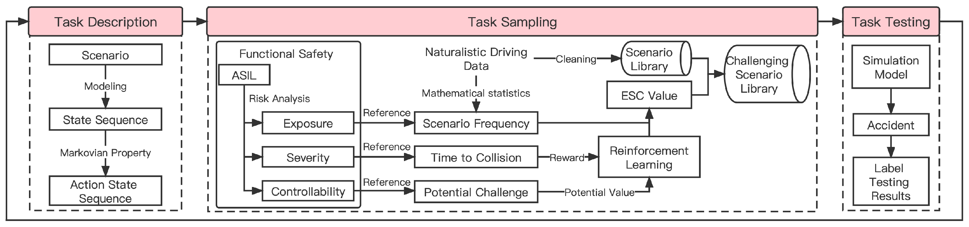
2. The Elementary Principle and Design of the Method
2.1. Functional Safety: Theoretical Basis
2.2. Quantification Method
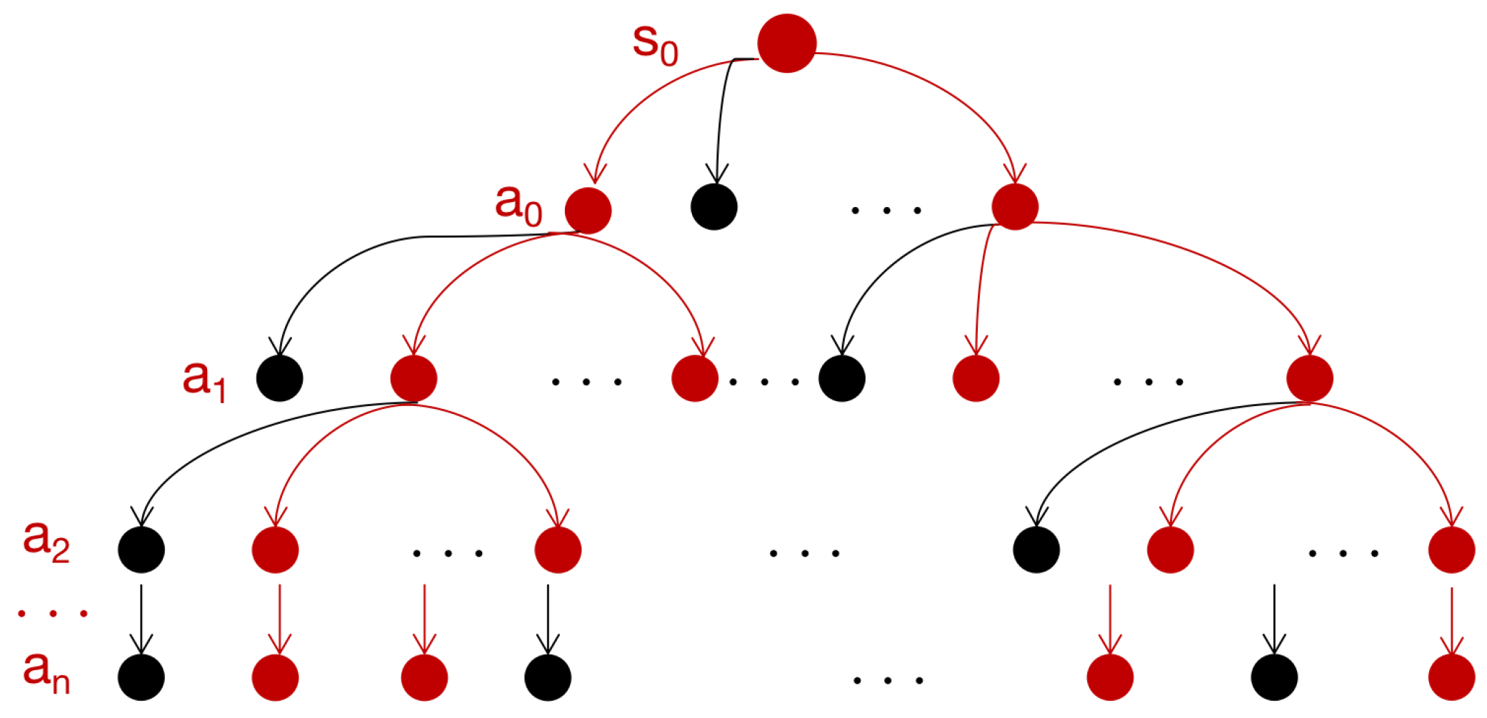
2.2.1. Scenario Modeling
- S is a set of states s of every agent.
- A is a discrete set of available agent actions that can be selected at a certain state.
- is the reward function that represents the reward gained from taking a certain action at a specific state.
- is the state transition probability matrix, which specifies the probability of taking action for a state. This is consistent with Markov Property, where the state transfer effect of taking action is only related to the current state, irrespective of the historical state.
- is the policy: SA, where the goal of RL is to learn the optimal policy to obtain the optimal expected reward.
2.2.2. Challenging Scenarios
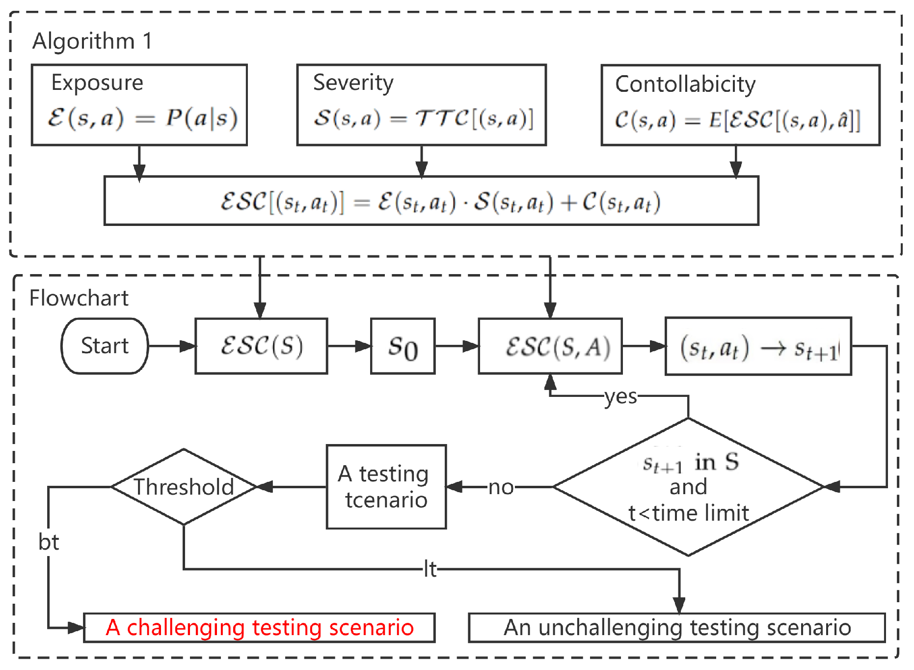
2.2.3. Quantification Analysis
- The value of is determined by naturalistic driving data (NDD) to reflect the probability of exposure. NDD describes the natural driving environment and can provide exposure information. By analyzing the samples in NDD, we can obtain the frequency of state as and the frequency of completing an action in the current state as . Therefore, can be defined as:
- The value of should reflect the level of severity of completing an action a in a current state s. As the direct consequence of completing an action in the current state leads to the next state, can be quantified by analyzing the next state caused by the action. As the definition is similar to reward function , the can be seen as the reward in exploration. Time to collision (TTC) is regarded as a useful metric to obtain the driver perception of collision risk [47] and was selected to evaluate the forward collision warning (FCW) warning threshold time. TTC is defined as Equation (6) [48] where is the related distance and is the related velocity. We quantified the severity according to TTC, as shown in Equation (7).
- The definition of differs from that of ISO26262, because controllability aimed at hazardous events focuses on external measures after traffic accidents, whereas testing aimed at scenarios does not. However, the primary goal considers the potential consequences and long-term challenge effects of the current state. Based on this, we defined as the expected from actions in the next state to reflect the long-term value of actions in the current state, as shown in Equation (8).
2.2.4. Algorithm
| Algorithm 1 . |
Initialize , , ; , ; ; while
do Initialize ; -; ; ; end while return
|
3. Experiments
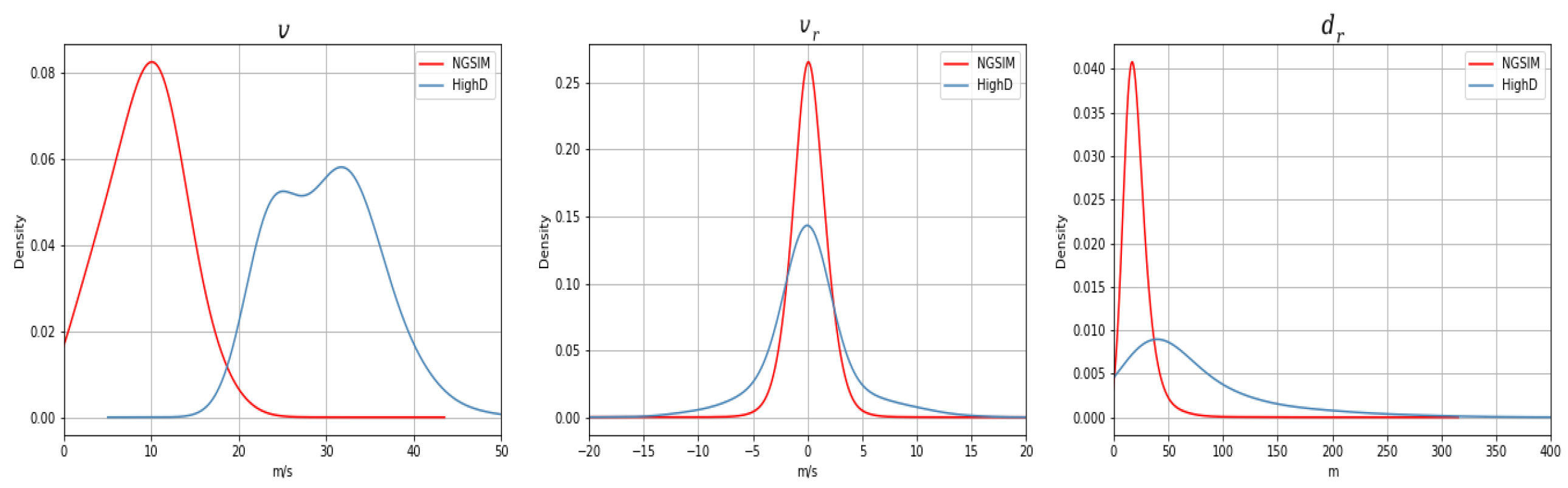
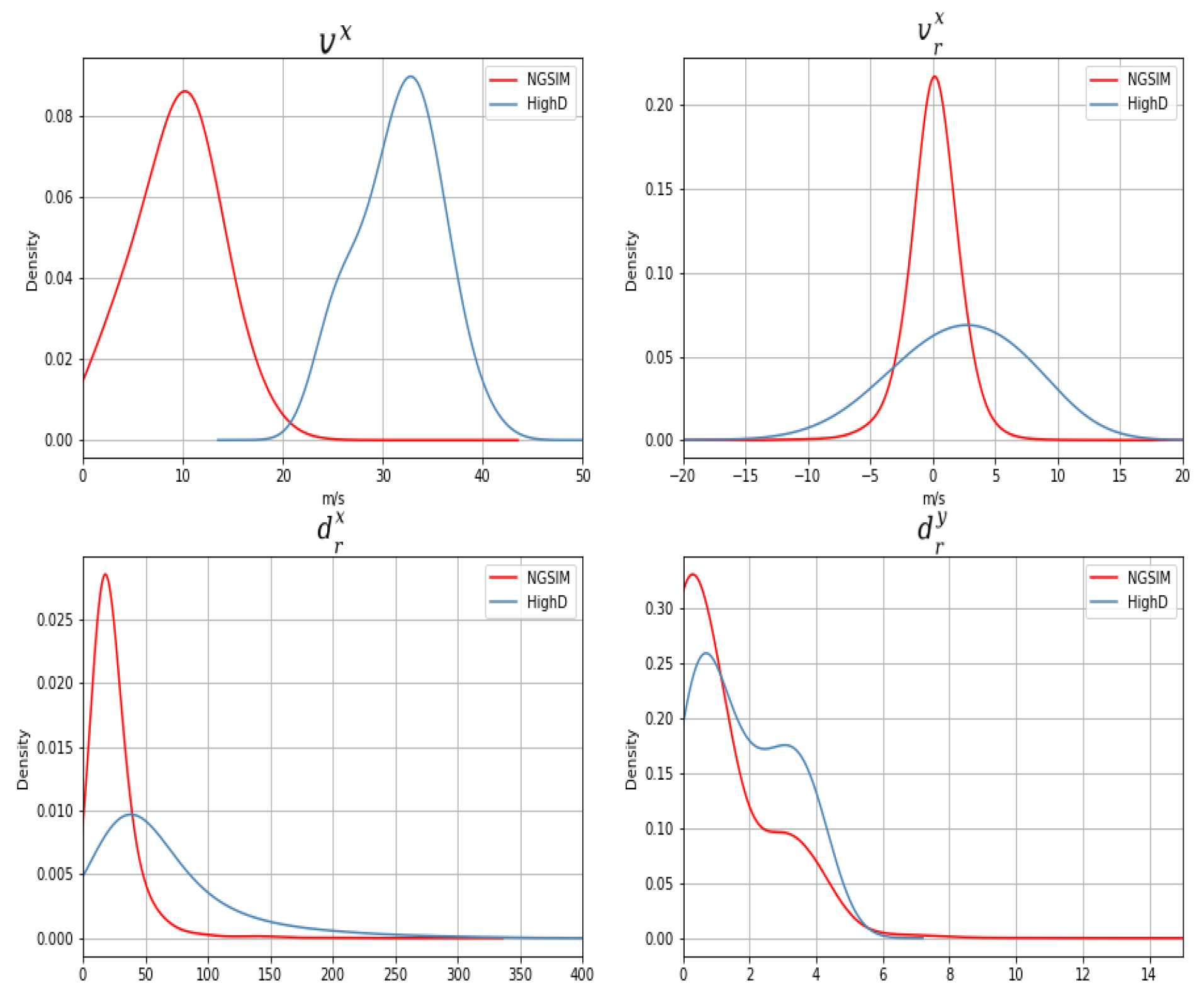
3.1. Dataset
3.2. Simulation Model
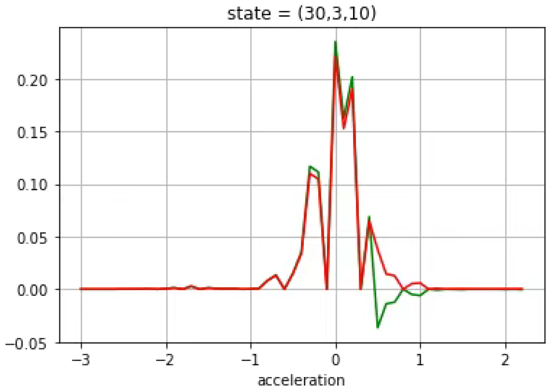
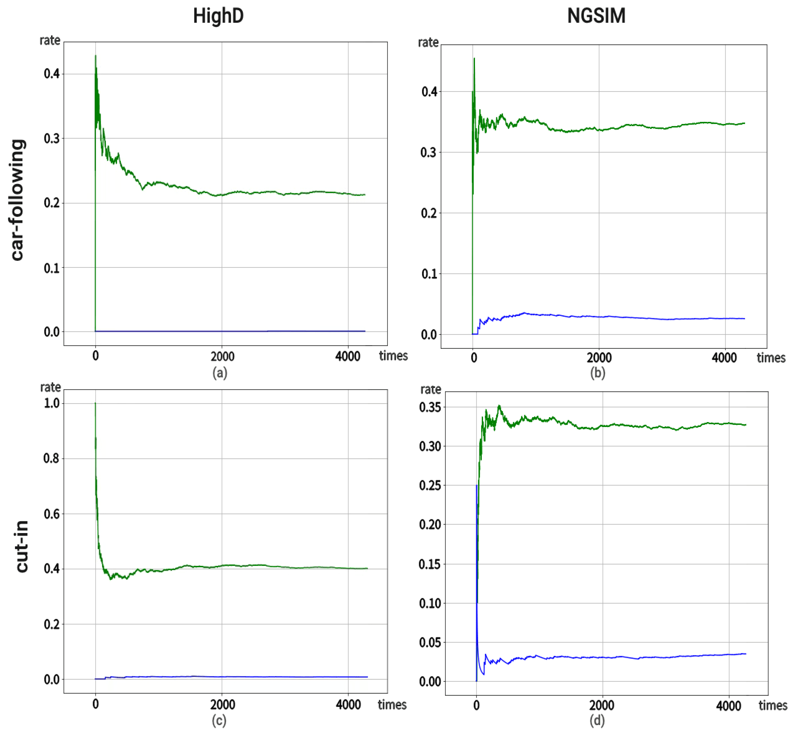
3.3. Car-Following Case
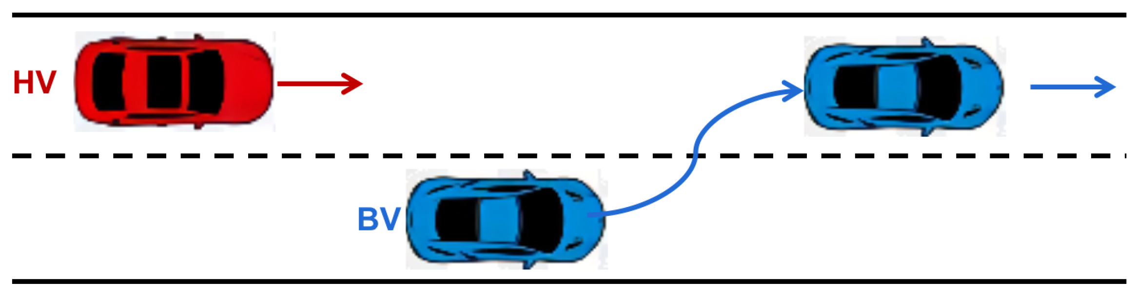
3.4. Cut-In Case
4. Analysis and Discussion
5. Conclusions
Author Contributions
Funding
Institutional Review Board Statement
Informed Consent Statement
Data Availability Statement
Acknowledgments
Conflicts of Interest
References
- Li, L.; Lin, Y.L.; Zheng, N.N.; Wang, F.Y.; Liu, Y.H.; Cao, D.P.; Wang, K.F.; Huang, W.L. Artificial intelligence test: A case study of intelligent vehicles. Artif. Intell. Rev. 2018, 50, 441–465. [Google Scholar] [CrossRef]
- Kalra, N.; Paddock, S.M. Driving to safety: How many miles of driving would it take to demonstrate autonomous vehicle reliability? Transp. Res. Part A Policy Pract. 2016, 94, 182–193. [Google Scholar] [CrossRef]
- Wang, F.Y.; Wang, X.J.; Li, L.; Mirchandani, P. Creating a Digital-Vehicle Proving Ground. IEEE Intell. Syst. 2003, 18, 12–15. [Google Scholar] [CrossRef]
- O’Kelly, M.; Sinha, A.; Namkoong, H.; Tedrake, R.; Duchi, J.C. Scalable End-to-End Autonomous Vehicle Testing via Rare-event Simulation. In Proceedings of the 32nd Conference on Neural Information Processing Systems (NeurIPS), Montréal, QC, Canada, 3–8 December 2018. [Google Scholar]
- Huang, W.L.; Wang, K.F.; Lv, Y.S.; Zhu, F.H. Autonomous vehicles testing methods review. In Proceedings of the IEEE 19th International Conference on Intelligent Transportation Systems (ITSC), Rio de Janeiro, Brazil, 1–4 November 2016. [Google Scholar]
- Chen, Y.; Chen, S.T.; Zhang, T.; Zhang, S.Y.; Zheng, N.N. Autonomous Vehicle Testing and Validation Platform: Integrated Simulation System with Hardware in the Loop. In Proceedings of the 29th IEEE Intelligent Vehicles Symposium (IV), Changshu, China, 26–30 June 2018. [Google Scholar]
- Kang, H.; Chen, Y.; Zhao, H. Construction of typical vehicle use environment based on virtual simulation test. J. Phys. Conf. Ser. 2018, 1576, 12054. [Google Scholar] [CrossRef]
- Koopman, P. Challenges in autonomous vehicle validation: Keynote presentation abstract. In Proceedings of the 1st International Workshop on Safe Control of Connected and Autonomous Vehicles, Pittsburgh, PA, USA, 18–21 April 2017; p. 3. [Google Scholar]
- Riedmaier, S.; Ponn, T.; Ludwig, D.; Schick, B.; Diermeyer, F. Survey on scenario-based safety assessment of automated vehicles. IEEE Access 2020, 8, 87456–87477. [Google Scholar] [CrossRef]
- Ulbrich, A.; Menzel, T.; Reschka, A.; Schuldt, F.; Maurer, M. Defining and Substantiating the Terms Scene, Situation, and Scenario for Automated Driving. In Proceedings of the 18th IEEE International Conference on Intelligent Transportation Systems (ITSC), Gran Canaria, Spain, 15–18 September 2015. [Google Scholar]
- Xia, Q.; Duan, J.; Gao, F.; Hu, Q.; He, Y. Test scenario design for intelligent driving system ensuring coverage and effectiveness. Int. J. Automot. Technol. 2018, 19, 751–758. [Google Scholar] [CrossRef]
- Duan, J.L.; Gao, F.; He, Y.D. Test scenario generation and optimization technology for intelligent driving systems. IEEE Intell. Transp. Syst. Mag. 2022, 14, 115–127. [Google Scholar] [CrossRef]
- Huang, L.; Xia, Q.; Xie, F.; Xiu, H.L.; Shu, H. Study on the test scenarios of level 2 automated vehicles. In Proceedings of the 29th IEEE Intelligent Vehicles Symposium (IV), Changshu, China, 26–30 June 2018. [Google Scholar]
- Xie, F.; Chen, T.; Xia, Q.; Huang, L.; Shu, H. Study on the controlled field test scenarios of automated vehicles. In Proceedings of the 2nd SAE Intelligent and Connected Vehicles Symposium (ICVS), Kunshan, China, 14–15 August 2018. [Google Scholar]
- Hu, X.; Zhu, B.; Tan, D.; Zhang, N.; Wang, Z. Test scenario generation method for autonomous vehicles based on combinatorial testing and bayesian network. Proc. Inst. Mech. Eng. Part J. Automob. Eng. 2022. [Google Scholar] [CrossRef]
- Zhao, D.; Peng, H.; Lam, H.; Bao, S.; Nobukawa, K.; LeBlanc, D.J.; Pan, C.S. Accelerated evaluation of automated vehicles in lane change scenarios. In Proceedings of the ASME 8th Annual Dynamic Systems and Control Conference, Columbus, OH, USA, 20–30 October 2015; Volume 57243, p. V001T17A002. [Google Scholar]
- Zhao, D.; Huang, X.; Peng, H.; Lam, H.; Leblanc, D.J. Accelerated evaluation of automated vehicles in car-following maneuvers. IEEE Trans. Intell. Transp. Syst. 2017, 19, 733–744. [Google Scholar] [CrossRef]
- Zhao, D.; Lam, H.; Peng, H.; Bao, S.; Leblanc, D.J.; Nobukawa, K.; Pan, C.S. Accelerated evaluation of automated vehicles safety in lane-change scenarios based on importance sampling technique. In Proceedings of the 20th IEEE International Conference on Intelligent Transportation Systems, Yokohama, Japan, 16–19 October 2017. [Google Scholar]
- Guo, H.; Zhang, J.; Liu, J.; Hu, Y.; Shi, W. Generation of a Scenario Library for Testing driver-automation Cooperation Safety under Cut-in Working Conditions. Green Energy Intell. Transp. 2022, 1, 100004. [Google Scholar] [CrossRef]
- Wang, Y.; Gong, J.; Wang, B.; Jia, P.; Kyo, T. Off-road testing scenario design and library generation for intelligent vehicles. Green Energy Intell. Transp. 2022, 1, 100013. [Google Scholar] [CrossRef]
- Li, N.; Kolmanovsky, I.; Girard, A. Model-free optimal control based automotive control system falsification. In Proceedings of the American Control Conference(ACC), Seattle, WA, USA, 24–26 May 2017. [Google Scholar]
- Chou, G.; Sahin, Y.E.; Yang, L.; Rutledge, K.J.; Nilsson, P.; Ozay, N. Using control synthesis to generate corner cases: A case study on autonomous driving. IEEE Trans. -Comput.-Aided Des. Integr. Circuits Syst. 2018, 37, 2906–2917. [Google Scholar] [CrossRef]
- Tian, H.; Jiang, Y.; Wu, G.; Yan, J.; Wei, J.; Chen, W.; Li, S.; Ye, D. Mosat: Finding safety violations of autonomous driving systems using multi-objective genetic algorithm. In Proceedings of the 30th ACM Joint European Software Engineering Conference and Symposium on the Foundations of Software Engineering, Singapore, 14–18 November 2022; pp. 94–106. [Google Scholar]
- Zhang, Y.; Sun, B.; Zhai, Y.; Li, Y.; Liang, H.; Liu, Q. Machine learning based testing scenario space and its safety boundary evaluation for automated vehicles. J. Phys. Conf. Ser. 2022, 2337, 012017. [Google Scholar] [CrossRef]
- Abeysirigoonawardena, Y.; Shkurti, F.; Dudek, G. Generating adversarial driving scenarios in high-fidelity simulators. In Proceedings of the 2019 IEEE International Conference on Robotics and Automation (ICRA), Montreal, BC, Canada, 20–24 May 2019. [Google Scholar]
- Zhou, R.; Lin, Z.; Huang, X.; Peng, J.; Huang, H. Testing scenarios construction for connected and automated vehicles based on dynamic trajectory clustering method. In Proceedings of the IEEE 25th International Conference on Intelligent Transportation Systems (ITSC), Macao, China, 8–12 October 2022. [Google Scholar]
- Xu, Z.; Bai, Y.; Wang, G.; Gan, C.; Sun, Y. Research on scenarios construction for automated driving functions field test. J. Phys. Conf. Ser. 2022, 2283, 012010. [Google Scholar] [CrossRef]
- Tuncali, C.E.; Fainekos, G. Rapidly-exploring random trees for testing automated vehicles. In Proceedings of the IEEE 22nd International Conference on Intelligent Transportation Systems (ITSC), Auckland, New Zealand, 27–30 October 2019. [Google Scholar]
- Koschi, M.; Pek, C.; Maierhofer, S.; Althoff, M. Computationally efficient safety falsification of adaptive cruise control systems. In Proceedings of the IEEE 22nd International Conference on Intelligent Transportation Systems (ITSC), Auckland, New Zealand, 27–30 October 2019. [Google Scholar]
- Lee, R.; Kochenderfer, M.J.; Mengshoel, O.J.; Brat, G.P.; Owen, M.P. Adaptive stress testing of airborne collision avoidance systems. In Proceedings of the IEEE/AIAA 34th Digital Avionics Systems Conference (DASC), Liverpool, UK, 13–18 September 2015. [Google Scholar]
- Koren, M.; Alsaif, S.; Lee, R.; Kochenderfer, M.J. Adaptive stress testing for autonomous vehicles. In Proceedings of the29th IEEE Intelligent Vehicles Symposium (IV), Changshu, China, 26–30 June 2018. [Google Scholar]
- Corso, A.; Du, P.; Driggs-Campbell, K.; Kochenderfer, M.J. Adaptive stress testing with reward augmentation for autonomous vehicle Validatio. In Proceedings of the IEEE 22nd International Conference on Intelligent Transportation Systems (ITSC), Auckland, New Zealand, 27–30 October 2019. [Google Scholar]
- Koren, M.; Kochenderfer, M.J. Efficient autonomy validation in simulation with adaptive stress testing. In Proceedings of the IEEE 22nd International Conference on Intelligent Transportation Systems (ITSC), Auckland, New Zealand, 27–30 October 2019. [Google Scholar]
- Feng, S.; Feng, Y.; Sun, H.; Bao, S.; Zhang, Y.; Liu, H.X. Testing scenario library generation for connected and automated vehicles, part II: Case studies. IEEE Trans. Intell. Transp. Syst. 2020, 22, 5635–5647. [Google Scholar] [CrossRef]
- Feng, S.; Feng, Y.; Yu, C.; Zhang, Y.; Liu, H.X. Testing scenario library generation for connected and automated vehicles, part I: Methodology. IEEE Trans. Intell. Transp. Syst. 2020, 22, 1573–1582. [Google Scholar] [CrossRef]
- Qin, X.; Arechiga, N.; Best, A.; Deshmukh, J. Automatic testing and falsification with dynamically constrained reinforcement learning. arXiv 2019, arXiv:1910.13645. [Google Scholar]
- Versaci, M.; Angiulli, G.; Crucitti, P.; Carlo, D.D.; Laganà, F.; Pellicanò, D.; Palumbo, A. A Fuzzy Similarity-Based Approach to Classify Numerically Simulated and Experimentally Detected Carbon Fiber-Reinforced Polymer Plate Defects. Sensors 2022, 22, 4232. [Google Scholar] [CrossRef]
- Alaei, A.; Pal, S.; Pal, U.; Blumenstein, M. An Efficient Signature Verification Method Based on an Interval Symbolic Representation and a Fuzzy Similarity Measure. IEEE Trans. Inf. Forensics Secur. 2017, 12, 2360–2372. [Google Scholar] [CrossRef]
- Tang, X.; Jiao, L.C.; Emery, W.J. SAR Image Content Retrieval Based on Fuzzy Similarity and Relevance Feedback. IEEE J. Sel. Top. Appl. Earth Obs. Remote Sens. 2017, 10, 1824–1842. [Google Scholar] [CrossRef]
- Kramer, B.; Neurohr, C.; Büker, M.; Böde, E.; Fränzle, M.; Damm, W. Identification and quantification of hazardous scenarios for automated driving. In Proceedings of the 7th International Symposium on Model-Based Safety and Assessment (IMBSA), Lisbon, Portugal, 14–16 September 2020. [Google Scholar]
- Sutton, R.; Barto, A. Reinforcement Learning: An introduction; MIT Press: Cambridge, MA, USA, 2018. [Google Scholar]
- ISO 26262; Road Vehicles—Functional Safety. I. O. for Standardization: London, UK, 2009.
- Ross, H.L. Functional Safety for Road Vehicles: New Challenges and Solutions for E-Mobility and Automated Driving; Springer: Berlin/Heidelberg, Germany, 2018. [Google Scholar]
- Gheraibia, Y.; Kabir, S.; Djafri, K.; Krimou, H. An Overview of the Approaches for Automotive Safety Integrity Levels Allocation. J. Fail. Anal. Prev. 2018, 18, 707–720. [Google Scholar] [CrossRef]
- Nardi, A.; Armato, A. Functional safety methodologies for automotive applications. In Proceedings of the 36th International Conference on Computer Aided Design (ICCAD), Irvine, CA, USA, 13–16 November 2017. [Google Scholar]
- Andersson, S.A.; Madigan, D.; Perlman, M.D. An alternative Markov property for chain graphs. Uncertain. Artif. Intell. 2013, 28, 33–85. [Google Scholar] [CrossRef]
- Lee, D.N. A theory of visual control of braking based on information about time-to-collision. Perception 1976, 5, 437–459. [Google Scholar] [CrossRef]
- Hydén, C. Traffic conflicts technique: State-of-the-art. In Traffic Safety Work with Video Processing; Topp, H.H., Ed.; Univ. of Kaiserslautern: Kaiserslautern, Germany, 1996; pp. 3–14. [Google Scholar]
- You, C.; Lu, J.; Filev, D.P.; Tsiotras, P. AHighway traffic modeling and decision making for autonomous vehicle using reinforcement learning. In Proceedings of the 29th IEEE Intelligent Vehicles Symposium (IV), Changshu, China, 26–30 June 2018. [Google Scholar]
- Hasselt, H.V.; Guez, A.; Silver, D. Deep Reinforcement Learning with Double Q-learning. In Proceedings of the 30th National Conference on Artificial Intelligence (AAAI), Phoenix, CA, USA, 12–17 February 2016. [Google Scholar]
- Geramifard, A.; Walsh, T.J.; Tellex, S.; Chowdhary, G.; Roy, N. A Tutorial on Linear Function Approximators for Dynamic Programming and Reinforcement Learning. Found. Trends Mach. Learn. 2013, 6, 375–451. [Google Scholar] [CrossRef]
- Krajewski, R.; Bock, J.; Kloeker, L.; Eckstein, L. The highD Dataset: A Drone Dataset of Naturalistic Vehicle Trajectories on German Highways for Validation of Highly Automated Driving Systems. In Proceedings of the IEEE 21st International Conference on Intelligent Transportation Systems (ITSC), Maui, HI, USA, 4–7 November 2018. [Google Scholar]
- Punzo, D.V.; Borzacchiello, M.T.; Ciuffo, B. On the assessment of vehicle trajectory data accuracy and application to the Next Generation SIMulation (NGSIM) program data. Transp. Res. Part Emerg. Technol. 2011, 19, 1243–1262. [Google Scholar] [CrossRef]
- Prabhakaran, N.; Sudhakar, M.S. Fuzzy curvilinear path optimization using fuzzy regression analysis for mid vehicle collision detection and avoidance system analyzed on NGSIM I-80 dataset (real-road scenarios). Neural Comput. Appl. 2019, 31, 1405–1423. [Google Scholar] [CrossRef]
- Treiber, M.; Hennecke, A.; Helbing, D. Congested Traffic States In Empirical Observations And Microscopic Simulations. Phys. Rev. E Stat. Phys. Plasmas Fluids, Relat. Interdiscip. Top. 2000, 2, 62. [Google Scholar] [CrossRef]
- Ahmed, H.U.; Huang, Y.; Lu, P. A review of car-following models and modeling tools for human and autonomous-ready driving behaviors in micro-simulation. Smart Cities 2021, 4, 314–335. [Google Scholar] [CrossRef]
- Feng, S.; Yan, X.; Sun, H.; Feng, Y.; Liu, H.X. Intelligent driving intelligence test for autonomous vehicles with naturalistic and adversarial environment. Nat. Commun. 2021, 12, 748. [Google Scholar] [CrossRef]


| Severity Class | Exposure Class | Controllability Class | ||
|---|---|---|---|---|
| C1 | C2 | C3 | ||
| S1 | E1 | QM | QM | QM |
| E2 | QM | QM | QM | |
| E3 | QM | QM | A | |
| E4 | QM | A | B | |
| S2 | E1 | QM | QM | QM |
| E2 | QM | QM | A | |
| E3 | QM | A | B | |
| E4 | A | B | C | |
| S3 | E1 | QM | QM | A |
| E2 | QM | A | B | |
| E3 | A | B | C | |
| E4 | B | C | D | |
| Parameter (HighD) | v (m/s) | (m/s) | (m) | a (m/) |
|---|---|---|---|---|
| maximum | 50 | 17 | 391 | 2.2 |
| minimum | 20 | −18 | 4 | −3.0 |
| Parameter (NGSIM) | v (m/s) | (m/s) | (m) | a (m/) |
| maximum | 29 | 20 | 210 | 3.4 |
| minimum | 0 | −19 | 2 | −3.4 |
| Parameter | Weight_HighD | Weight_NGSIM | Interpretation |
|---|---|---|---|
| a | 2.2 | 3.4 | maximum acceleration |
| b | −3 | −3.4 | minimum acceleration |
| 33 | 33 | desired velocity | |
| 4 | 4 | acceleration velocity | |
| L | 4 | 2 | vehicle length |
| 2 | 2 | gap at jam conditions | |
| 0 | 0 | gap factor | |
| T | 1 | 1 | the reaction time of driver |
| Parameter (HighD) | ||||||
|---|---|---|---|---|---|---|
| unit | (m/s) | (m/s) | (m) | (m) | (m/) | (m/s) |
| maximum | 42 | 16 | 345 | 5 | 1.9 | 1.8 |
| minimum | 23 | −19 | 0 | 0 | −1.1 | 0.1 |
| Parameter (NGSIM) | ||||||
| unit | (m/s) | (m/s) | (m) | (m) | (m/) | (m/s) |
| maximum | 29 | 17 | 224 | 13 | 3.4 | 2.0 |
| minimum | 0 | −15 | 2 | 0 | −3.4 | 0.0 |
Disclaimer/Publisher’s Note: The statements, opinions and data contained in all publications are solely those of the individual author(s) and contributor(s) and not of MDPI and/or the editor(s). MDPI and/or the editor(s) disclaim responsibility for any injury to people or property resulting from any ideas, methods, instructions or products referred to in the content. |
© 2023 by the authors. Licensee MDPI, Basel, Switzerland. This article is an open access article distributed under the terms and conditions of the Creative Commons Attribution (CC BY) license (https://creativecommons.org/licenses/by/4.0/).
Share and Cite
Meng, K.; Zhou, R.; Li, Z.; Zhang, K. A Quantitative Approach of Generating Challenging Testing Scenarios Based on Functional Safety Standard. Appl. Sci. 2023, 13, 3494. https://doi.org/10.3390/app13063494
Meng K, Zhou R, Li Z, Zhang K. A Quantitative Approach of Generating Challenging Testing Scenarios Based on Functional Safety Standard. Applied Sciences. 2023; 13(6):3494. https://doi.org/10.3390/app13063494
Chicago/Turabian StyleMeng, Kang, Rui Zhou, Zhiheng Li, and Kai Zhang. 2023. "A Quantitative Approach of Generating Challenging Testing Scenarios Based on Functional Safety Standard" Applied Sciences 13, no. 6: 3494. https://doi.org/10.3390/app13063494
APA StyleMeng, K., Zhou, R., Li, Z., & Zhang, K. (2023). A Quantitative Approach of Generating Challenging Testing Scenarios Based on Functional Safety Standard. Applied Sciences, 13(6), 3494. https://doi.org/10.3390/app13063494