Abstract
Recently, various metaheuristic (MH) optimization algorithms have been presented and applied to solve complex engineering and optimization problems. One main category of MH algorithms is the naturally inspired swarm intelligence (SI) algorithms. SI methods have shown great performance on different problems. However, individual MH and SI methods face some shortcomings, such as trapping at local optima. To solve this issue, hybrid SI methods can perform better than individual ones. In this study, we developed a boosted version of the reptile search algorithm (RSA) to be employed for different complex problems, such as intrusion detection systems (IDSs) in cloud–IoT environments, as well as different optimization and engineering problems. This modification was performed by employing the operators of the red fox algorithm (RFO) and triangular mutation operator (TMO). The aim of using the RFO was to boost the exploration of the RSA, whereas the TMO was used for enhancing the exploitation stage of the RSA. To assess the developed approach, called RSRFT, a set of six constrained engineering benchmarks was used. The experimental results illustrated the ability of RSRFT to find the solution to those tested engineering problems. In addition, it outperformed the other well-known optimization techniques that have been used to handle these problems.
1. Introduction
In daily life, optimization is everywhere. Optimization is used widely in many fields, including system management, technical design, economics, and various engineering problems [1,2]. To optimize something means to make sure one or more goals of a particular situation are as ideal as possible. The goal of the optimization process is to investigate potential solutions and find the optimal one. Occasionally, many constraints are applied to solutions, making optimization more difficult [3].
In recent decades, the effectiveness of metaheuristic (MH) techniques in solving complicated problems with high dimensionality, multimodality, and non-differentiability has been proven by different studies in different applications [4,5,6]. As a result, the use of these algorithms has increased significantly, and there is a growing trend to suggest efficient upgrades and new metaheuristic algorithms. These algorithms primarily gain their inspiration from natural phenomena, physics laws, animals’ and birds’ behaviors, and so on. Earlier, some efficient optimization algorithms were developed, such as the genetic algorithm (GA) [7], artificial bee colony (ABC) [8], particle swarm optimization (PSO) [9], and the firefly algorithm [10]. Recently, there have been many newly developed metaheuristic optimization algorithms based on different inspirations, for example the sine–cosine algorithm (SCA) [11], the multi-verse optimizer (MVO) [12], Harris hawks optimization (HHO) [13], the marine predator algorithm [14], the Aquila optimizer [15], the arithmetic optimization algorithm [16], the Reptile search algorithm (RSA) [17], and many other optimization techniques.
Although those algorithms have shown good performance in different optimization and engineering algorithms, in some cases, they face critical limitations and shortcomings. According to the well-known no free lunch theorem, no one method has the ability of solving all problems. To this end, in recent years, researchers have used the hybridization concept to develop hybrid metaheuristic optimization algorithms to address different engineering and optimization issues.
For example, Houssein et al. [3] applied an improved equilibrium optimizer (EO) using a technique called the self-adaptive EO algorithm. They used four search techniques to enhance the search process of the EO optimization method. This method was employed to address different optimization engineering problems, and it showed better results compared to the original EO. Bo et al. [18] applied several search techniques, namely opposition-based learning and greedy search, to boost the chimp optimization algorithm (ChOA) search mechanism. The developed ChOA was employed to solve different constrained engineering problems and recorded significant outcomes. Shen et al. [19] introduced an enhanced whale optimization algorithm (WOA) to handle engineering design problems and global optimization issues. They used a technique called multi-population evolution to improve the original WOA. A modified SCA was developed by Yang et al. [20]. They suggested a multi-mechanism acting SCA method to overcome the drawbacks of the original SCA. This modified version of the SCA was utilized to address constrained engineering optimization problems. An improved SSA optimization technique was developed by Hong et al. [21] to solve engineering problems, using a new strategy called producer centralization. Furthermore, in [22], a modified improved moth–flame optimizer was suggested using two search mechanisms, namely Gaussian mutation and chaotic grouping. This modified method was evaluated with complex engineering and optimization problems. An enhanced FA was suggested by Peng et al. [23] to solve complex engineering optimization problems. They applied three search techniques to enhance the traditional FA. Zhang et al. [24] presented a modified AOA to be employed in various numerical and engineering optimization applications based on two techniques, called random high-speed jumping and multi-leader wandering around search strategy. Hybrid optimization algorithms have also been adopted in other research areas, such as a hybrid of AO and the seagull optimization algorithm for wind power forecasting [25] and a hybrid of AO with the SMA and SSO to predict CO2 trapping in deep saline [26,27]. Another hybrid optimization method was developed by [28] using DE and the Cuckoo Search algorithm to optimize the ship pipe route. Moreover, a hybrid method of HHO and DE was suggested by Zhong et al. to solve the flight trajectory prediction problem [29].
In recent years, MH optimization techniques also have been investigated to address the problems of intrusion detection systems. Many optimization algorithms have been suggested as feature selection methods to improve the quality solutions of the IDS, such as PSO [30], the GA [31], AO [32], HHO [33], and many other approaches [1,2].
Paper Contribution
Inspired by the successful applications of the hybrid concept to overcome the drawbacks of the individual optimization algorithms, in this study, we present a new version of the reptile search algorithm using two techniques, namely the red fox optimization algorithm and the mutation operators. The RSA [17] is a recently developed optimization method emulating crocodiles’ hunting behaviors in nature. It has been adopted in various applications since it has high performance, such as in [34,35,36]. The red fox optimization algorithm [37] is also a nature-inspired technique based on the hunting behavior of the red fox. It has also been adopted in solving some optimization problems [38,39,40].
The main modification was performed using RFO to enhance the ability of the RSA to explore the search domain. Additionally, the triangular mutation operator (TMO) was applied to improve the exploitation of the RSA. This competition between the operators of the RSA, TMO, and RFO led to enhancing the rate of convergence toward the optimal solution.
In short, we can represent the contributions of this study as the following points:
- We propose a boosted version of the reptile search algorithm (RSA), called RSRFT, to address IDS problems in IoT and cloud environments, as well as complex and multidimensional engineering problems
- We employed the operators of the red fox optimization and triangular mutation operator to boost the performance of the RSA.
- We applied the RSRFT technique to solve different and complex engineering problems. We conducted a set of comparisons with other efficient techniques to verify the quality of RSRFT.
The rest of this study is organizes as follows: In Section 2, detailed background descriptions of the applied algorithms are presented. Section 3 introduces the descriptions of the RSRFT approach. In Section 4, we assess the quality of the modified RSA method using different datasets and with extensive comparisons to other methods, and in Section 5, we present the conclusion of this paper.
2. Background
2.1. The Reptile Search Algorithm
The conventional RSA, which simulates actual crocodile behavior, is presented in this section. This was accomplished using two steps: the local and global search stages.
2.1.1. Exploration Search
Following [17], the process of splitting the maximum number of generations into four parts will trigger the RSA to switch from the exploration to the exploitation stage. Moreover, the RSA exploration phase investigates the search domains using two primary search techniques in pursuit of a more reliable agent. There are two requirements for this search component. If the long walking plan is not adjusted by t ≤ , the agents are modified by t ≤ 2 and t > . Equation (1) can be utilized to update the positions for the exploration stage:
where stands for the best solution at dimension j. denotes the value of a randomly selected solution at dimension j. represents a random value, and as in [17]. T represents the total number of generations. N and are the number of solutions and the hunting operator. The definition of is given as
In Equation (4), refers to a small value. is a random integer value, while is defined as
In Equation (5), and represent the boundaries of the search domain, and [17]. M() denotes the mean value of X, and it is given as
2.1.2. Exploitation Search
Using the hunting coordination plan, t ≤ 3 and t > adopt the agents in this stage. In contrast, if t ≤ T and t > 3, the hunting cooperation plan is carried out. Equation (7) provides the updated value using the exploitation process.
2.2. Red Fox Algorithm
This optimizer begins by figuring out the parameters’ values and then creating the population of N foxes according to Equation (8):
where and indicate the boundaries of the search space, while D represents the dimension of foxes. Thereafter, the objective value of is evaluated then allocating the best solution . The next process is to update using the following formula:
In Equation (9), stands for a scaling hyperparameter chosen randomly, whereas is defined as
In case has a fitness value better than its previous value, then we replace with . Otherwise, we preserved the value. The observation radius r is then adjusted by applying the formula Equation (11) in the case of the fox not being seen:
In Equation (11), is a random value that is applied to control adverse weather conditions such as fog, rain, etc. After that, X is updated based on the following formula:
where and each angular value represents a randomized one for each point.
This set of equations simulates a fox’s actions after it spots a target and tries to attack it. Then, the fitness value of is assessed and then sorted based on the values. Hunters may kill the worst solution, while Equation (13) is employed to update the X solution.
where in the first branch of Equation (13); the new solutions wander outside the environment in search of a new space to repopulate their herd as nomadic agents. Outside of the habitat and within the search zone, the solution is chosen randomly. The center of the habitat () is calculated as
In Equation (14), and denote the first- and second-best solutions, respectively.
2.3. Triangular Mutation Operator
The mutation technique utilizes a integration vector, which is constructed using three randomly selected vectors along with three distinct vectors that have been selected during the competition (the best, worst, and better). This combination vector is then utilized to create the new mutant vector.
In Equation (16), and refer to the mutation factors that are related to and they are produced according to the uniform distribution. In addition, three tournaments are given as , , . In addition, is the combination vector triangle at iteration t and formulated as:
where is a real weight and is formulated as .
Moreover, the mutation is used to balance the exploitation propensity with the exploration capacity, with the primary mutation favoring the exploration phase. As a result, utilizing the presented mutation is twice as likely to succeed as using the fundamental principles. The differential evolution (DE) method is the foundation of the advanced mutation technique. Thus, using the fundamental mutation approach DE/rand/1/bin, the following new combination is created:
If, then
Else:
In Equation (18), F is a random value at and a random value.
3. Proposed RSRFT Method
Within this section, we introduce the stages of the developed technique, which depends on modifying the performance of the RSA using TMO and RFO as given in Figure 1. The main objective of RFO is to facilitate the identification of a feasible solution within the feasible area, while TMO is applied to promote harmony between the exploitation and exploration. The initial population of RSRFT is constructed inside the search space’s confines. The best solution is then selected from the current population after the fitness function for each solution has been evaluated. The solutions are updated using the RSA, RFO, and TMO operators. The RFO technique will then be used to update a collection of individuals that have reached a local standstill. Until the terminal condition is satisfied, the updating of the population is conducted again. The next subsections offer a detailed explanation of the developed RSRFT approach.
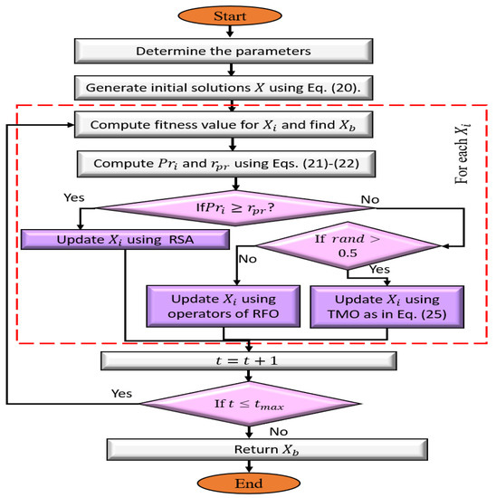
Figure 1.
Developed RSRFT approach.
3.1. Initial Phase
The RSRFT creates the N agent starting populations as
3.2. Updating Phase
The current X is updated by using either the operators of the RSA, RFO, or TMO. This can be conducted through a set of steps. The first step is to calculate the fitness value for . The smallest fitness value and its related solution are then identified. Then, according to the probability of the fitness value, either the operators of the RSA or RFO and TMO are used to update X. This probability is computed as
Then, the updating is performed using the following formula:
where is computed as
In addition, the value of is computed as
while the values of and refer to the updated value of using the operators of RFO and the RSA, respectively.
3.3. Terminal Phase
The stopping conditionsare examined during this phase, and in case they are satisfied, the steps of updating are halted and is returned. Otherwise, a new updating step is carried out.
The main steps of the proposed RSRFT are given in Algorithm 1.
| Algorithm 1 The RSRFT method. |
|
4. Experimental Results and Discussion
In this study, the performance of RSRFT was evaluated through two experimental series, which included engineering problems and improve the security in the IoT environment. The experiments illustrated in this section were conducted using MATLAB R2020b installed on machine configured with a 2.40 GHz Intel Core i5 CPU, 4.00 GB RAM, and a Windows 10 operating system.
4.1. Series of Analysis 1: Engineering Problems
The evaluation of the developed RSRFT to solve the constraint optimization engineering problem is presented in this section. Six engineering optimization problems—the design of welded beams, the design of tension/compression springs, and the design optimization challenge for pressure vessels—were the focus of this experiment. The next subsections address the problem definition and results.
4.1.1. Welded Beam Design Problem
Determining the welding beam’s settings that lower the fabrication costs are the major goal of solving welded beam design (WBD) problem (Figure 2). These parameters are the bar’s height (t), the length of an attached portion (l), the weld’s thickness (h), and the bar’s thickness (b).
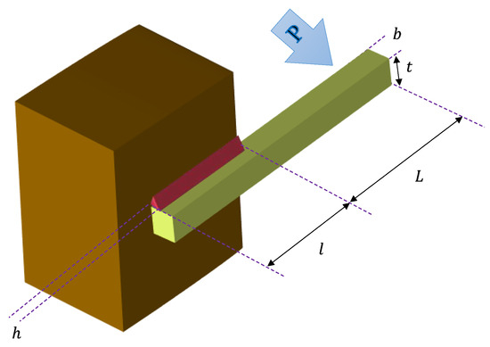
Figure 2.
Structure of the WBD problem.
The definition of WBD is formulated as
RSRFT was compared to several optimization techniques, such as the whale optimization algorithm (WOA) [41], MVO [12], evolutionary particle swarm optimization (CPSO) [42], LSHcEpS [43], co-evolutionary differential evolution (CSCA) [44], the simplex method (SIMPLEX) [45], Davidon–Fletcher–Powell (DAVID) [45], the gravitational search algorithm (GSA) [46], the GA [47], harmony search (HS) [48], and LSHADE_SPACMA (we renamed it as LSHSPCM) [49]. The developed RSRFT was conducted for 25 independent runs with and .
Table 1 contains the results of RSRFT and the compared optimization techniques. The RSRFT technique had the lowest cost (as given in the column Optimal Objective), followed by LSHSPCM, while SIMPLEX had the highest cost. As a result, the design parameters obtained by RSRFT were more suitable for WBD.

Table 1.
The value of the estimated parameters using RSRFT and other methods for solving the WBD problem.
4.1.2. Tension/Compression Spring Design Problem
Within this section, we evaluated the performance of RSRFT to allocate the parameters that are used to minimize spring weight during tension/compression spring design (TCSD), which is defined in Figure 3. Those parameters include the wire diameter (d), the mean coil diameter (D), and the number of active coils (N) of a spring. The formulation of TCSD is illustrated as
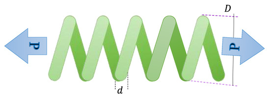
Figure 3.
Design of the TCSD problem.
In this experiment, RSRFT was compared with other approaches that have been used to solve the TCSD problem, for example CPSO [42], MVO [12], the GA [52], the GSA [41], the evolution strategy (ES) [53], the Ray–Saini method [54], the WOA [41], the CSCA [44], the method proposed by Belegundu and Arora [55], LSHSPCM, and LSHcEpS. The results of the comparison between RSRFT and the others are given in Table 2. The RSRFT offered superior outcomes over the other methods.
Table 2.
The value of the estimated parameters using RSRFT and others to solve the TCSD problem.
4.1.3. Pressure Vessel Design Problem
This section presents the performance of developed RSRFT to solve another engineering problem, named the pressure vessel design (PVD) problem (see Figure 4), by determining the parameters that lead to minimizing the cost of the pressure cylinder. Those parameters are the thickness of the head , the length of the cylindrical section of the vessel L, the thickness , and the inner radius R. The mathematical representation of PVD is given as
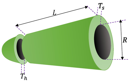
Figure 4.
Schematic of the PVD problem.
The outcomes of the comparisons are listed in Table 3. Those approaches are HPSO [56], ACO [57], the ES [53], the GA [52], PSO-DE [58], the GSA [41], CDE [44], and LSHSPCM [49]. From these results, we noticed that RSRFT was able to reach the minimum objective value (as given in the column Optimal Objective), which outperformed the other compared techniques.
Table 3.
The value of the estimated parameters using RSRFT and other approaches to solve the PVD problem.
4.1.4. Three-Bar Truss Design Problem Design
The major aim of Three-Bar Truss Design (TBTD) is to minimize the weight of the structure [59,60]. Figure 5 illustrates the geometry structure of TBTD, in which cross-sectional areas stand in for the design variables. The cross-section with and must be found according to [59] because of the system’s symmetry. Below is a diagram that represents the TBTD problem mathematically.

Figure 5.
The three-bar truss design problem.
RSRFT was used to allocate the design variables. Furthermore, we compared RSRFT to other methods used to address the TBTD problem, which are shown in Table 4. Since RSRFT obtained the smallest weight (as given under Optimal Weight), it is clear from the findings in this table that it offered the best solution. However, the outcomes of the traditional RSA were better than the competitive algorithms, including RSRFT.
Table 4.
The value of the estimated parameters using RSRFT to solve the 3-bar truss design problem.
4.1.5. Speed Reducer Problem
In order for an airplane’s propeller and engine to rotate at an efficient speed, a gearbox between them is needed (see Figure 6 [67]). The optimization strategy employed to address the speed reducer problem is intended for minimizing the design’s weight while still meeting the requirements for the bending stress of the gear teeth, surface stress, transverse shaft deflections, and stresses in the shafts. The best value for each of the seven design factors must be established to solve this problem.

Figure 6.
The speed reducer problem.
These variables are the face width (), the module of the teeth (), the number of teeth on the pinion (), the lengths of the first and second shafts between the bearings ( and , respectively), the first shaft’s diameter ( and , respectively), and the module of the teeth (). Given that it contains more limitations than other issues, the speed reducer problem is defined as having a high degree of complexity. Below is a diagram that represents this issue mathematically.
Table 5 provides the comparative findings between RSRFT and the other MH approaches that have been given in the literature. It is clear that RSRFT surpassed the majority of the techniques that were examined (as given under Optimal Weight), and it was generally assigned the third rank. CS and SBSM were assigned the first and second ranks, respectively [64,68]. Since all three algorithms almost had the same ideal weight, there was little difference between them.
Table 5.
The value of the estimated parameters using RSRFT to solve the speed reducer design problem.
4.1.6. Multiple Disc Clutch Brake Problem
Finding the values of five design factors to reduce the mass of an MDCB is the primary goal of research into the multiple disc clutch brake (MDCB) problem, which was cited in [63]. The design parameters are shown in Figure 7 as the inner radius , outer radius , disc thickness , actuation force , and number of friction surfaces . Below is a diagram that represents this issue mathematically.
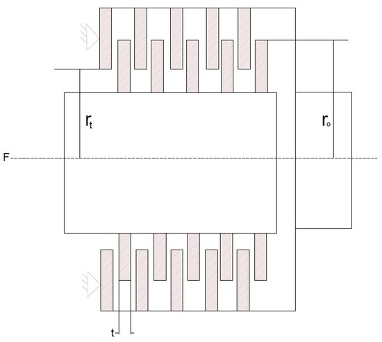
Figure 7.
The multiple disc clutch brake problem.
Table 6 lists the outcomes of RSRFT and other MH approaches collected from the literature. From this table, it is clear that RSRFT obtained the ideal cost (0.31176) (as given under Optimal Weight), which was then followed by CMVO, MFO, MVO, and the WCA, which had the same efficiency.
Table 6.
The value of the estimated parameters using RSRFT to solve the multiple disc clutch brake problem.
4.2. Series of Analysis 2: RSRFT for Security in the IoT
Within this section, we evaluated the applicability of RSRFT to improve the detection of IDSs in the IoT environment [81]. In general, the problem definition of IDSs in the Internet of Things (IoT) is the need to detect and prevent unauthorized access, data breaches, and malicious activities in IoT devices and networks. With the rapid growth of the IoT, there has been an increase in the number and complexity of connected devices, which has also led to an increase in the number of potential attack vectors and vulnerabilities. As a result, there is a growing need for effective IDSs that can identify and respond to these threats in real-time [82].
The challenge of developing IDSs for the IoT is the complexity of the networks and the diversity of the devices. The systems need to be designed to detect and respond to a wide range of attack types, including malware, denial-of-service attacks, and insider threats. Furthermore, the systems need to be able to identify anomalous behaviors and patterns that may indicate an attack, while also avoiding false positives [83].
To address this problem, we present an alternative technique to detect the intrusions in the IoT. In this experiment, RSRFT was used as a feature selection technique to enhance the process of selecting the important features of the collected data in the IoT environment. This can be achieved through by the Boolean version of RSRFT by converting the real value of each solution into a binary value.
The proposed RSRFT starts by generating the value of the initial population. This can be defined as
where and are the upper and lower boundaries, respectively. In this experiment, the values of and , while . This step is followed by obtaining the binary of using the following formula:
The next process is to assess the quality of the selected features, which correspond to the ones in , using the following formula.
where denotes the classification error of the KNN classifier, whereas the term refers to the ratio of features selected using . The value of is applied as the weight of the two terms of Equation (34).
Thereafter, according to the fitness values, we determined the best of them and their corresponding solution . Then, we used this solution and the operators of RSRFT that are discussed in Section 3.2 and Section 3.3 to update X. The next step after reaching the stop conditions is to compute the efficiency of using the testing set of IoT data.
In the following sections, we introduce the datasets used in this experiment to assess RSRFT as an FS method. The comparison was conducted with moth–flame optimization (MFO) [60], the bat (BAT) algorithm [84], transient search optimization (TSO) [83], and the RSA. The parameter of each approach was assigned based on the original implementation.
4.2.1. Dataset Description
The proposed algorithm was assessed using the KDDCup-99, NSL-KDD, BoT-IoT, and CICIDS-2017 datasets. The KDD-99 dataset, created by the Defense Advanced Research Project Agency (DARPA) in 1988, contains network traffic data. Another kind of dataset, called NSL-KDD, was also used, which is a derived dataset with no duplicate network traffic records and grouped into four types: Probe, U2R, R2L, and DoS, in addition to normal data. The CICIDS-2017 dataset [85] was obtained from 25 clients at the Canadian Institute for Cybersecurity (CIC) using the CICFlowMeter tool to simulate realistic network traffic obtained using protocols such as HTTP, SSH, HTTPS, FTP, and email. Additionally, the Bot-IoT dataset [86] includes 3.5 million records produced from different IoT devices and features botnet attacks.The description of all of these datasets is given in Table 7.
Table 7.
Description of the datasets.
4.2.2. Evaluation Criteria and Experimental Setup
In this study, various performance and evaluation criteria were applied to evaluate the effectiveness of RSRFT, including the average accuracy , the average recall , and the average precision :
- : This stands for the rate of the correct detection of intrusions in the IoT environment. can be formulated aswhere is the total number of runs. FN, TN, TP, and FP refer to false negative, true negative, true positive, and false positive, respectively.
- : This can also be referred to as the true positive rate, and it describes the percentage of correctly predicted positive intrusions. is computed as
- : This describes the ratio of true detections among all correct detection samples, and it is formulated as
4.2.3. Results and Discussion
The performance of the enhanced RSA based on TMO and RFO as the feature selection technique to improve the detection of IDSs in the IoT environment is discussed in this section. Table 8 shows the average results of the developed RSRFT to improve the detection of IDSs in the IoT environment using the training and testing sets. From these results, it can be noticed that RSRFT had a high ability to improve the detection of the IDSs in terms of accuracy. In addition, it can be observed that the behavior of RFO alone was the worst one among the tested algorithms using the training and testing sets. According to the results of the precision, recall, and F1-measure, it can be noticed that the developed algorithm was the first-ranked algorithm. This indicated that the ability of the developed RSRFT was better than exploring and exploiting the search space.
Table 8.
Results of RSRFT for improving the detection of IDSs in the IoT environment.
Figure 8 and Figure 9 show the average accuracy, precision, F1-measure, and recall using the training and testing sets, respectively. From these figures, we can see that the average of each measure (i.e., accuracy, precision, F1-measure, and recall) of RSRFT was better than that of the other methods using the training and testing sets. This was followed by the RSA, which provided better results than the other methods.
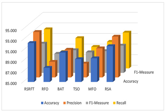
Figure 8.
Performance measures of RSRFT using the training set.

Figure 9.
Performance measures of RSRFT using the testing set.
Moreover, we used the Friedman test as a non-parametric test to assess if there was a significant difference between the developed RSRFT and the others. Table 9 shows the mean rank obtained using each approach over the training and testing sets and among the performance measures. From these results, it can be noticed that the developed RSRFT had the highest mean rank, and the difference between it and the others was significant since the p-value was less than 0.05, except for the precision value using the training set.
Table 9.
The mean rank using the Friedman test.
From the previous results of the two experimental series, it can be observed that the developed RSRFT had high efficiency to determine the solution of different engineering problems, whereas we noticed the high ability of RSRFT to enhance the process of improving the detection of IDSs in the IoT environment by reducing the number of selected features. This resulted from boosting the operators of the RSA, RFO, and TMO to improve the rate of convergence towards the optimal solution. However, there are some limitations in RSRFT, for example the initial population can influence the performance of the developed method. In addition, the diversity of the solutions needs more improvement.
5. Conclusions
In this paper, the use of an enhanced version of the reptile search algorithm (RSA) to solve engineering problems was shown to be a highly effective approach. By combining the strengths of the RSA with those of the red fox algorithm (RFO) and triangular mutation operator (TMO), this modification was able to effectively explore a wider range of possible solutions and find improved solutions more quickly. The results of this study demonstrated the effectiveness of the developed approach, named RSRFT, in solving a variety of engineering problems and showed that this algorithm can provide reliable and accurate solutions in a variety of contexts. Overall, the use of RSRFT represents a promising advancement in the field of engineering and has the potential to greatly improve the design and optimization of various systems and technologies. In the second experiment series, we evaluated RSRFT as a feature selection method to improve the classification of intrusion detection systems (IDSs) in the IoT and cloud environments. Four IDS datasets were utilized to test the performance of RSRFT, namely, KDD99, NSL-KDD, BIoT, and CIC2017. The results also confirmed the superiority of RSRFT.
In future works, the presented RSRFT can be extended to other areas, including task scheduling in cloud and fog environments, medical applications, agriculture, and others. Additionally, it may be tested on multi-objective optimization problems and solar cell parameter estimation.
Author Contributions
All authors contributed equally to this work. All authors have read and agreed to the published version of the manuscript.
Funding
This research project was funded by the Deanship of Scientific Research, Princess Nourah bint Abdulrahman University, through the Program of Research Project Funding After Publication, grant No. (43- PRFA-P-24).
Data Availability Statement
All of the datasets are public, as we described in the main texts.
Acknowledgments
This research project was funded by the Deanship of Scientific Research, Princess Nourah bint Abdulrahman University, through the Program of Research Project Funding After Publication, grant No (43- PRFA-P-24).
Conflicts of Interest
The authors declare no conflict of interest.
Nomenclature
| Acronyms | |
| IDS | Intrusion detection system |
| IoT | Internet of Things |
| MH | Metaheuristic |
| RFO | Red fox algorithm |
| RSA | Reptile search algorithm |
| TMO | Triangular mutation operator |
| Variables | |
| Combination vector triangle | |
| Hunting operator | |
| Best solution | |
| M() | Mean value of X |
| N | Number of solutions |
| t | Iteration |
| X | Population |
| Value of randomly selected solution | |
References
- Sarkar, A.; Guchhait, R.; Sarkar, B. Application of the artificial neural network with multithreading within an inventory model under uncertainty and inflation. Int. J. Fuzzy Syst. 2022, 24, 2318–2332. [Google Scholar]
- Sarkar, B.; Takeyeva, D.; Guchhait, R.; Sarkar, M. Optimized radio-frequency identification system for different warehouse shapes. Knowl.-Based Syst. 2022, 258, 109811. [Google Scholar]
- Houssein, E.H.; Çelik, E.; Mahdy, M.A.; Ghoniem, R.M. Self-adaptive Equilibrium Optimizer for solving global, combinatorial, engineering, and Multi-Objective problems. Expert Syst. Appl. 2022, 195, 116552. [Google Scholar]
- Abualigah, L.; Ewees, A.A.; Al-qaness, M.A.; Elaziz, M.A.; Yousri, D.; Ibrahim, R.A.; Altalhi, M. Boosting arithmetic optimization algorithm by sine cosine algorithm and levy flight distribution for solving engineering optimization problems. Neural Comput. Appl. 2022, 34, 8823–8852. [Google Scholar]
- Al-Qaness, M.A.; Helmi, A.M.; Dahou, A.; Elaziz, M.A. The applications of metaheuristics for human activity recognition and fall detection using wearable sensors: A comprehensive analysis. Biosensors 2022, 12, 821. [Google Scholar] [PubMed]
- Al-Qaness, M.A.; Ewees, A.A.; Abualigah, L.; AlRassas, A.M.; Thanh, H.V.; Abd Elaziz, M. Evaluating the Applications of Dendritic Neuron Model with Metaheuristic Optimization Algorithms for Crude-Oil-Production Forecasting. Entropy 2022, 24, 1674. [Google Scholar] [PubMed]
- Whitley, D. A genetic algorithm tutorial. Stat. Comput. 1994, 4, 65–85. [Google Scholar]
- Dorigo, M.; Di Caro, G. Ant colony optimization: A new meta-heuristic. In Proceedings of the 1999 Congress on Evolutionary Computation-CEC99 (Cat. No. 99TH8406), Washington, DC, USA, 6–9 July 1999; Volume 2, pp. 1470–1477. [Google Scholar]
- Kennedy, J.; Eberhart, R. Particle swarm optimization. In Proceedings of the ICNN’95-International Conference on Neural Networks, Perth, WA, Australia, 27 November–1 December 1995; Volume 4, pp. 1942–1948. [Google Scholar]
- Yang, X.S.; Slowik, A. Firefly algorithm. In Swarm Intelligence Algorithms; CRC Press: Boca Raton, FL, USA, 2020; pp. 163–174. [Google Scholar]
- Mirjalili, S. SCA: A sine cosine algorithm for solving optimization problems. Knowl.-Based Syst. 2016, 96, 120–133. [Google Scholar]
- Mirjalili, S.; Mirjalili, S.M.; Hatamlou, A. Multi-verse optimizer: A nature-inspired algorithm for global optimization. Neural Comput. Appl. 2016, 27, 495–513. [Google Scholar]
- Heidari, A.A.; Mirjalili, S.; Faris, H.; Aljarah, I.; Mafarja, M.; Chen, H. Harris hawks optimization: Algorithm and applications. Future Gener. Comput. Syst. 2019, 97, 849–872. [Google Scholar]
- Faramarzi, A.; Heidarinejad, M.; Mirjalili, S.; Gandomi, A.H. Marine Predators Algorithm: A nature-inspired metaheuristic. Expert Syst. Appl. 2020, 152, 113377. [Google Scholar]
- Abualigah, L.; Yousri, D.; Abd Elaziz, M.; Ewees, A.A.; Al-Qaness, M.A.; Gandomi, A.H. Aquila optimizer: A novel meta-heuristic optimization algorithm. Comput. Ind. Eng. 2021, 157, 107250. [Google Scholar]
- Abualigah, L.; Diabat, A.; Mirjalili, S.; Abd Elaziz, M.; Gandomi, A.H. The arithmetic optimization algorithm. Comput. Methods Appl. Mech. Eng. 2021, 376, 113609. [Google Scholar]
- Abualigah, L.; Abd Elaziz, M.; Sumari, P.; Geem, Z.W.; Gandomi, A.H. Reptile Search Algorithm (RSA): A nature-inspired meta-heuristic optimizer. Expert Syst. Appl. 2022, 191, 116158. [Google Scholar]
- Bo, Q.; Cheng, W.; Khishe, M. Evolving chimp optimization algorithm by weighted opposition-based technique and greedy search for multimodal engineering problems. Appl. Soft Comput. 2023, 132, 109869. [Google Scholar]
- Shen, Y.; Zhang, C.; Gharehchopogh, F.S.; Mirjalili, S. An Improved Whale Optimization Algorithm based on Multi-Population Evolution for Global Optimization and Engineering Design problems. Expert Syst. Appl. 2023, 215, 119269. [Google Scholar]
- Yang, X.; Wang, R.; Zhao, D.; Yu, F.; Huang, C.; Heidari, A.A.; Cai, Z.; Bourouis, S.; Algarni, A.D.; Chen, H. An adaptive quadratic interpolation and rounding mechanism sine cosine algorithm with application to constrained engineering optimization problems. Expert Syst. Appl. 2023, 213, 119041. [Google Scholar]
- Hong, J.; Shen, B.; Xue, J.; Pan, A. A vector-encirclement-model-based sparrow search algorithm for engineering optimization and numerical optimization problems. Appl. Soft Comput. 2022, 131, 109777. [Google Scholar]
- Zhao, X.; Fang, Y.; Ma, S.; Liu, Z. Multi-swarm improved moth–flame optimization algorithm with chaotic grouping and Gaussian mutation for solving engineering optimization problems. Expert Syst. Appl. 2022, 204, 117562. [Google Scholar]
- Peng, H.; Xiao, W.; Han, Y.; Jiang, A.; Xu, Z.; Li, M.; Wu, Z. Multi-strategy firefly algorithm with selective ensemble for complex engineering optimization problems. Appl. Soft Comput. 2022, 120, 108634. [Google Scholar]
- Zhang, Y.J.; Wang, Y.F.; Yan, Y.X.; Zhao, J.; Gao, Z.M. LMRAOA: An improved arithmetic optimization algorithm with multi-leader and high-speed jumping based on opposition-based learning solving engineering and numerical problems. Alex. Eng. J. 2022, 61, 12367–12403. [Google Scholar]
- Al-qaness, M.A.; Ewees, A.A.; Elaziz, M.A.; Samak, A.H. Wind Power Forecasting Using Optimized Dendritic Neural Model Based on Seagull Optimization Algorithm and Aquila Optimizer. Energies 2022, 15, 9261. [Google Scholar]
- Al-qaness, M.A.; Ewees, A.A.; Thanh, H.V.; AlRassas, A.M.; Dahou, A.; Elaziz, M.A. Predicting CO2 trapping in deep saline aquifers using optimized long short-term memory. Environ. Sci. Pollut. Res. 2022, 1–15. [Google Scholar] [CrossRef]
- Al-qaness, M.A.; Ewees, A.A.; Thanh, H.V.; AlRassas, A.M.; Abd Elaziz, M. An optimized neuro-fuzzy system using advance nature-inspired Aquila and Salp swarm algorithms for smart predictive residual and solubility carbon trapping efficiency in underground storage formations. J. Energy Storage 2022, 56, 106150. [Google Scholar]
- Lin, Y.; Bian, X.Y.; Dong, Z.R. A discrete hybrid algorithm based on Differential Evolution and Cuckoo Search for optimizing the layout of ship pipe route. Ocean. Eng. 2022, 261, 112164. [Google Scholar]
- Zhong, X.; You, Z.; Cheng, P. A hybrid optimization algorithm and its application in flight trajectory prediction. Expert Syst. Appl. 2023, 213, 119082. [Google Scholar]
- Balyan, A.K.; Ahuja, S.; Lilhore, U.K.; Sharma, S.K.; Manoharan, P.; Algarni, A.D.; Elmannai, H.; Raahemifar, K. A hybrid intrusion detection model using ega-pso and improved random forest method. Sensors 2022, 22, 5986. [Google Scholar] [PubMed]
- Bu, S.J.; Kang, H.B.; Cho, S.B. Ensemble of Deep Convolutional Learning Classifier System Based on Genetic Algorithm for Database Intrusion Detection. Electronics 2022, 11, 745. [Google Scholar]
- Fatani, A.; Dahou, A.; Al-Qaness, M.A.; Lu, S.; Abd Elaziz, M. Advanced feature extraction and selection approach using deep learning and Aquila optimizer for IoT intrusion detection system. Sensors 2022, 22, 140. [Google Scholar]
- Mansour, R.F. Blockchain assisted clustering with Intrusion Detection System for Industrial Internet of Things environment. Expert Syst. Appl. 2022, 207, 117995. [Google Scholar]
- Dahou, A.; Abd Elaziz, M.; Chelloug, S.A.; Awadallah, M.A.; Al-Betar, M.A.; Al-qaness, M.A.; Forestiero, A. Intrusion Detection System for IoT Based on Deep Learning and Modified Reptile Search Algorithm. Comput. Intell. Neurosci. 2022, 2022, 6473507. [Google Scholar]
- Elgamal, Z.; Sabri, A.Q.M.; Tubishat, M.; Tbaishat, D.; Makhadmeh, S.N.; Alomari, O.A. Improved Reptile Search Optimization Algorithm using Chaotic map and Simulated Annealing for Feature Selection in Medical Filed. IEEE Access 2022, 10, 51428–51446. [Google Scholar] [CrossRef]
- Chauhan, S.; Vashishtha, G.; Kumar, A. Approximating parameters of photovoltaic models using an amended reptile search algorithm. J. Ambient. Intell. Humaniz. Comput. 2022, 1–16. [Google Scholar] [CrossRef]
- Połap, D.; Woźniak, M. Red fox optimization algorithm. Expert Syst. Appl. 2021, 166, 114107. [Google Scholar]
- Khorami, E.; Mahdi Babaei, F.; Azadeh, A. Optimal diagnosis of COVID-19 based on convolutional neural network and red Fox optimization algorithm. Comput. Intell. Neurosci. 2021, 2021, 4454507. [Google Scholar] [PubMed]
- Natarajan, R.; Megharaj, G.; Marchewka, A.; Divakarachari, P.B.; Hans, M.R. Energy and Distance Based Multi-Objective Red Fox Optimization Algorithm in Wireless Sensor Network. Sensors 2022, 22, 3761. [Google Scholar]
- Zaborski, M.; Woźniak, M.; Mańdziuk, J. Multidimensional Red Fox meta-heuristic for complex optimization. Appl. Soft Comput. 2022, 131, 109774. [Google Scholar]
- Mirjalili, S.; Lewis, A. The whale optimization algorithm. Adv. Eng. Softw. 2016, 95, 51–67. [Google Scholar]
- Krohling, R.A.; dos Santos Coelho, L. Coevolutionary particle swarm optimization using Gaussian distribution for solving constrained optimization problems. IEEE Trans. Syst. Man Cybern. Part B (Cybern.) 2006, 36, 1407–1416. [Google Scholar]
- Awad, N.H.; Ali, M.Z.; Suganthan, P.N. Ensemble sinusoidal differential covariance matrix adaptation with Euclidean neighborhood for solving CEC2017 benchmark problems. In Proceedings of the 2017 IEEE Congress on Evolutionary Computation (CEC), San Sebastián, Spain, 5–8 June 2017; pp. 372–379. [Google Scholar]
- Huang, F.z.; Wang, L.; He, Q. An effective co-evolutionary differential evolution for constrained optimization. Appl. Math. Comput. 2007, 186, 340–356. [Google Scholar]
- Ragsdell, K.; Phillips, D. Optimal design of a class of welded structures using geometric programming. J. Manuf. Sci. Eng. 1976, 38, 1021–1025. [Google Scholar]
- Rashedi, E.; Nezamabadi-Pour, H.; Saryazdi, S. GSA: A gravitational search algorithm. Inf. Sci. 2009, 179, 2232–2248. [Google Scholar]
- Deb, K. Optimal design of a welded beam via genetic algorithms. AIAA J. 1991, 29, 2013–2015. [Google Scholar]
- Lee, K.S.; Geem, Z.W. A new meta-heuristic algorithm for continuous engineering optimization: Harmony search theory and practice. Comput. Methods Appl. Mech. Eng. 2005, 194, 3902–3933. [Google Scholar]
- Mohamed, A.W.; Hadi, A.A.; Fattouh, A.M.; Jambi, K.M. LSHADE with semi-parameter adaptation hybrid with CMA-ES for solving CEC 2017 benchmark problems. In Proceedings of the 2017 IEEE Congress on Evolutionary Computation (CEC), San Sebastián, Spain, 5–8 June 2017; pp. 145–152. [Google Scholar]
- Ewees, A.A.; Abd Elaziz, M.; Houssein, E.H. Improved grasshopper optimization algorithm using opposition-based learning. Expert Syst. Appl. 2018, 112, 156–172. [Google Scholar]
- Kaveh, A.; Khayatazad, M. A new meta-heuristic method: Ray optimization. Comput. Struct. 2012, 112, 283–294. [Google Scholar]
- Coello, C.A.C. Use of a self-adaptive penalty approach for engineering optimization problems. Comput. Ind. 2000, 41, 113–127. [Google Scholar]
- Mezura-Montes, E.; Coello, C.A.C. An empirical study about the usefulness of evolution strategies to solve constrained optimization problems. Int. J. Gen. Syst. 2008, 37, 443–473. [Google Scholar]
- Ray, T.; Saini, P. Engineering design optimization using a swarm with an intelligent information sharing among individuals. Eng. Optim. 2001, 33, 735–748. [Google Scholar]
- Belegundu, A.D.; Arora, J.S. A study of mathematical programmingmethods for structural optimization. Part II: Numerical results. Int. J. Numer. Methods Eng. 1985, 21, 1601–1623. [Google Scholar]
- He, Q.; Wang, L. A hybrid particle swarm optimization with a feasibility-based rule for constrained optimization. Appl. Math. Comput. 2007, 186, 1407–1422. [Google Scholar] [CrossRef]
- Kaveh, A.; Talatahari, S. An improved ant colony optimization for constrained engineering design problems. Eng. Comput. 2010, 27, 155–182. [Google Scholar] [CrossRef]
- Liu, H.; Cai, Z.; Wang, Y. Hybridizing particle swarm optimization with differential evolution for constrained numerical and engineering optimization. Appl. Soft Comput. 2010, 10, 629–640. [Google Scholar] [CrossRef]
- Ray, T.; Liew, K.M. Society and civilization: An optimization algorithm based on the simulation of social behavior. IEEE Trans. Evol. Comput. 2003, 7, 386–396. [Google Scholar] [CrossRef]
- Mirjalili, S. Moth-flame optimization algorithm: A novel nature-inspired heuristic paradigm. Knowl.-Based Syst. 2015, 89, 228–249. [Google Scholar] [CrossRef]
- Zhang, M.; Luo, W.; Wang, X. Differential evolution with dynamic stochastic selection for constrained optimization. Inf. Sci. 2008, 178, 3043–3074. [Google Scholar] [CrossRef]
- Mirjalili, S.; Gandomi, A.H.; Mirjalili, S.Z.; Saremi, S.; Faris, H.; Mirjalili, S.M. Salp Swarm Algorithm: A bio-inspired optimizer for engineering design problems. Adv. Eng. Softw. 2017, 114, 163–191. [Google Scholar] [CrossRef]
- Sadollah, A.; Bahreininejad, A.; Eskandar, H.; Hamdi, M. Mine blast algorithm: A new population based algorithm for solving constrained engineering optimization problems. Appl. Soft Comput. 2013, 13, 2592–2612. [Google Scholar] [CrossRef]
- Gandomi, A.H.; Yang, X.S.; Alavi, A.H. Cuckoo search algorithm: A metaheuristic approach to solve structural optimization problems. Eng. Comput. 2013, 29, 17–35. [Google Scholar] [CrossRef]
- YILDIRIM, A.E.; KARCI, A. Application of Three Bar Truss Problem among Engineering Design Optimization Problems using Artificial Atom Algorithm. In Proceedings of the 2018 International Conference on Artificial Intelligence and Data Processing (IDAP), Malatya, Turkey, 28–30 September 2018; pp. 1–5. [Google Scholar]
- Saremi, S.; Mirjalili, S.; Lewis, A. Grasshopper optimisation algorithm: Theory and application. Adv. Eng. Softw. 2017, 105, 30–47. [Google Scholar] [CrossRef]
- Siddall, J.N. Analytical Decision-Making in Engineering Design; Prentice Hall: Upper Saddle River, NJ, USA, 1972. [Google Scholar]
- Akhtar, S.; Tai, K.; Ray, T. A socio-behavioral simulation model for engineering design optimization. Eng. Optim. 2002, 34, 341–354. [Google Scholar] [CrossRef]
- SARUHAN, H.; UYGUR, İ. Design optimization of mechanical systems using genetic algorithms. Sak. Üniv. Fen Bilim. Enst. Derg. 2003, 7, 77–84. [Google Scholar]
- Geem, Z.W.; Kim, J.H.; Loganathan, G.V. A new heuristic optimization algorithm: Harmony search. Simulation 2001, 76, 60–68. [Google Scholar] [CrossRef]
- Mezura-Montes, E.; Coello, C.C.; Landa-Becerra, R. Engineering optimization using simple evolutionary algorithm. In Proceedings of the 15th IEEE International Conference on Tools with Artificial Intelligence, Sacramento, CA, USA, 5 November 2003; pp. 149–156. [Google Scholar]
- Lu, S.; Kim, H.M. A regularized inexact penalty decomposition algorithm for multidisciplinary design optimization problems with complementarity constraints. J. Mech. Des. 2010, 132, 410051–4100512. [Google Scholar] [CrossRef]
- Stephen, S.; Christu, D.; David, D.C.N. Design Optimization of Weight of Speed Reducer Problem Through Matlab and Simulation Using Ansys. Int. J. Mech. Eng. Technol. 2018, 9, 339–349. [Google Scholar]
- Baykasoğlu, A.; Ozsoydan, F.B. Adaptive firefly algorithm with chaos for mechanical design optimization problems. Appl. Soft Comput. 2015, 36, 152–164. [Google Scholar] [CrossRef]
- Kamboj, V.K.; Nandi, A.; Bhadoria, A.; Sehgal, S. An intensify Harris Hawks optimizer for numerical and engineering optimization problems. Appl. Soft Comput. 2020, 89, 106018. [Google Scholar] [CrossRef]
- Rao, R.V.; Savsani, V.J.; Vakharia, D. Teaching–learning-based optimization: A novel method for constrained mechanical design optimization problems. Comput.-Aided Des. 2011, 43, 303–315. [Google Scholar] [CrossRef]
- Deb, K.; Srinivasan, A. Innovization: Discovery of innovative design principles through multiobjective evolutionary optimization. In Multiobjective Problem Solving from Nature; Springer: Berlin/Heidelberg, Germany, 2008; pp. 243–262. [Google Scholar]
- Eskandar, H.; Sadollah, A.; Bahreininejad, A.; Hamdi, M. Water cycle algorithm—A novel metaheuristic optimization method for solving constrained engineering optimization problems. Comput. Struct. 2012, 110, 151–166. [Google Scholar] [CrossRef]
- Sayed, G.I.; Darwish, A.; Hassanien, A.E. A new chaotic multi-verse optimization algorithm for solving engineering optimization problems. J. Exp. Theor. Artif. Intell. 2018, 30, 293–317. [Google Scholar] [CrossRef]
- Bhesdadiya, R.; Trivedi, I.N.; Jangir, P.; Jangir, N. Moth-flame optimizer method for solving constrained engineering optimization problems. In Advances in Computer and Computational Sciences; Springer: Berlin/Heidelberg, Germany, 2018; pp. 61–68. [Google Scholar]
- Zarpelão, B.B.; Miani, R.S.; Kawakani, C.T.; de Alvarenga, S.C. A survey of intrusion detection in Internet of Things. J. Netw. Comput. Appl. 2017, 84, 25–37. [Google Scholar] [CrossRef]
- Abomhara, M.; Køien, G.M. Security and privacy in the Internet of Things: Current status and open issues. In Proceedings of the 2014 international conference on privacy and security in mobile systems (PRISMS), Aalborg, Denmark, 11–14 May 2014; pp. 1–8. [Google Scholar]
- Fatani, A.; Abd Elaziz, M.; Dahou, A.; Al-Qaness, M.A.; Lu, S. IoT intrusion detection system using deep learning and enhanced transient search optimization. IEEE Access 2021, 9, 123448–123464. [Google Scholar] [CrossRef]
- Yang, X.S. A new metaheuristic bat-inspired algorithm. In Nature Inspired Cooperative Strategies for Optimization (NICSO 2010); Springer: Berlin/Heidelberg, Germany, 2010; pp. 65–74. [Google Scholar]
- Koroniotis, N.; Moustafa, N.; Sitnikova, E.; Turnbull, B. Towards the development of realistic botnet dataset in the internet of things for network forensic analytics: Bot-iot dataset. Future Gener. Comput. Syst. 2019, 100, 779–796. [Google Scholar] [CrossRef]
- Sharafaldin, I.; Lashkari, A.H.; Ghorbani, A.A. Toward generating a new intrusion detection dataset and intrusion traffic characterization. ICISSp 2018, 1, 108–116. [Google Scholar]


Disclaimer/Publisher’s Note: The statements, opinions and data contained in all publications are solely those of the individual author(s) and contributor(s) and not of MDPI and/or the editor(s). MDPI and/or the editor(s) disclaim responsibility for any injury to people or property resulting from any ideas, methods, instructions or products referred to in the content. |
© 2023 by the authors. Licensee MDPI, Basel, Switzerland. This article is an open access article distributed under the terms and conditions of the Creative Commons Attribution (CC BY) license (https://creativecommons.org/licenses/by/4.0/).