Article

An Efficient Computational Approach for Inverse Kinematics Analysis of the UR10 Robot with SQP and BP-SQP Algorithms

1
School of Mechanical Engineering, Hubei University of Technology, Wuhan 430068, China
2
State Key Laboratory of Digital Manufacturing Equipment and Technology, Huazhong University of Science and Technology, Wuhan 430074, China
3
Dongfeng Liuzhou Motor Co., Ltd., Liuzhou 545005, China
*
Author to whom correspondence should be addressed.
Appl. Sci. 2023, 13(5), 3009; https://doi.org/10.3390/app13053009
Submission received: 11 February 2023 / Revised: 22 February 2023 / Accepted: 24 February 2023 / Published: 26 February 2023

Abstract

:
Two algorithms that are distinct from the closed algorithm are proposed to create the inverse kinematics model of the UR10 robot: the Sequential Quadratic Programming (SQP) algorithm and the Back Propagation-Sequential Quadratic Programming (BP-SQP) algorithm. The SQP algorithm is an iterative algorithm in which the fundamental tenet is that the joint’s total rotation radian should be at a minimum when the industrial robot reaches the target attitude. With this tenet, the SQP algorithm establishes the inverse kinematics model of the robot. Since the SQP algorithm is overly reliant on the initial values, deviations occur easily and the solution speed, and the accuracy of the algorithm is undermined. To assuage this disadvantage of the SQP algorithm, a BP-SQP algorithm incorporating a neural network is introduced to optimize the initial values. The results show that the SQP algorithm is an iterative algorithm that relies excessively on the initial values and has a narrow range of applications. The BP-SQP algorithm eliminates the limitations of the SQP algorithm, and the time complexity of the BP-SQP algorithm is greatly reduced. Subsequently, the effectiveness of the SQP algorithm and the BP-SQP algorithm is verified. The results show that the SQP and BP-SQP algorithms can significantly reduce the operation time compared with the closed algorithm, and the BP-SQP algorithm is faster but requires a certain number of samples as a prerequisite.

1. Introduction

In recent years, with the continuous development of science and technology, there have been more and more innovations in the traditional processing field, such as the use of industrial robots for processing, which can improve processing accuracy and efficiency [1,2,3,4,5]. However, the premise of using industrial robots for processing is to build the kinematics models of the robot [6,7]. The kinematics models of the robot are divided into two types, the forward kinematics model and the inverse kinematics model [8,9,10,11]. The traditional methods for solving the inverse kinematics of a robot are iterative, analytical, and geometric methods. Studies across the world have found that to utilize the closed algorithm to establish the inverse kinematics model of an industrial robot, the robot needs to meet either of the two criteria in Pieper [12] criteria, which are (1) three adjacent joint axes intersect at one point and (2) three adjacent joint axes are parallel to each other. However, many special industrial robots cannot meet the Pieper criteria, and therefore closed-form solutions based on the closed algorithm cannot be employed to resolve the inverse kinematics of the industrial robots [13,14,15,16,17]. The inverse kinematics algorithm based on matrix decomposition proposed by Liu, Songguo is an optimization algorithm that reduces the complexity of the existing inverse kinematics algorithms and solves the problem of root addition in the solution process [18]. Lü proposed a method to solve the inverse kinematics of a 6R robot with the spinor equation based on Wu’s method. The proposed algorithm by Lü, combined with the spinor method, successfully avoided the limitations of the sub-problem algorithm when the spinor method is utilized to solve the inverse kinematics of the 6R robot [19]. Liao proposed a method to solve inverse kinematics based on the iterative method, where the problem concerning how to solve inverse kinematics is converted into a problem of solving a nonlinear equation set. At the same time, in order to reduce the complexity, the converted problem is then transformed into an algorithm with traversal to resolve the kinematics [20]. Si et al. proposed a complete closed-form solution of inverse kinematics, discussed the existence of the offset and distance between the axis of the first joint and the axis of the second joint, and gave all possible solutions and singularity configurations [21]. Lin et al. proposed a combination of the geometric method and the analytical method to resolve inverse kinematics, which does not increase the calculation cost [22]. Zhang, Jintao et al. proposed a method that solves inverse kinematics based on angle parameterization of robotic arms to solve offset of links at the shoulders, elbows, and wrist joints of a class of redundant spatial robotic manipulators [23]. Yu et al. proposed that when the robot does not meet the Pieper criterion, a sequential transposition method based on adjacent joint axes can resolve the inverse kinematics model of the robot [24]. Li and Cui et al. proposed a closed vector loop method to solve the inverse kinematics model of a robotic mechanism [25,26]. Yang used the improved fruit fly optimization algorithm (IFOA) to reduce large amounts of calculation and increase precision in the process of solving inverse kinematics [27]. Xie et al. transformed the nonlinear equation for creating the inverse solution into an optimization problem that includes an objective function where a differential evolution algorithm is constructed by minimizing the deviations of the pose of the terminal end of a robot to resolve the robot’s inverse kinematic model [28]. Wang et al. proposed a painting algorithm that can generate a painting trajectory satisfying the painting of large objects by resolving the UR5 robot’s inverse kinematics [29]. Kucuk [30] proposed an effective iterative inverse kinematic algorithm NIKA and compared the simulation results with the Newton-Raphson algorithm to verify the good performance of the NIKA algorithm. Bingül et al. [31] used particle swarm optimization (PSO) and least squares (LS) methods to estimate the inertial parameters of the Staubli RX-60 robot, and experiments showed that the particle swarm algorithm outperformed the LS method for parameter estimation.
This paper, which mainly adopts the SQP (sequential quadratic programming) algorithm and BP-SQP (sequential quadratic programming based on back propagation neural network) algorithm, studies the inverse kinematics model of the UR10 robot. The SQP algorithm can solve nonlinear problems with constraints and reduce the complexity of the calculation. When establishing the inverse kinematics model of the UR10 robot, the SQP algorithm takes the minimum total rotation radians of the UR10 robot’s joints as the constraint condition. The SQP algorithm is highly dependent on the initial values and will cause deviations. The time the SQP algorithm needs to find a solution and the accuracy of the SQP algorithm are impacted. In order to eliminate the limitations of the SQP algorithm, we propose the BP-SQP algorithm. On the basis of the SQP algorithm, a neural network algorithm, which is called the BP-SQP algorithm, is introduced to optimize the initial values. The BP-SQP algorithm is based on the error backpropagation method. Through the training process, the weights and offsets are continuously adjusted to reduce errors. The judgment of the condition for terminating the propagation is that the current number of iterations is the predetermined maximum number of iterations or is lower than the allowable accuracy. The BP (backpropagation) neural network has great advantages in solving inverse kinematics. The operation speed is greatly improved. The SQP algorithm optimized by the BP neural network can find the best inverse solution faster. Finally, the effectiveness of the SQP and BP-SQP algorithms is verified by simulation experiments.

2. The Physical Model of the UR10 Robot

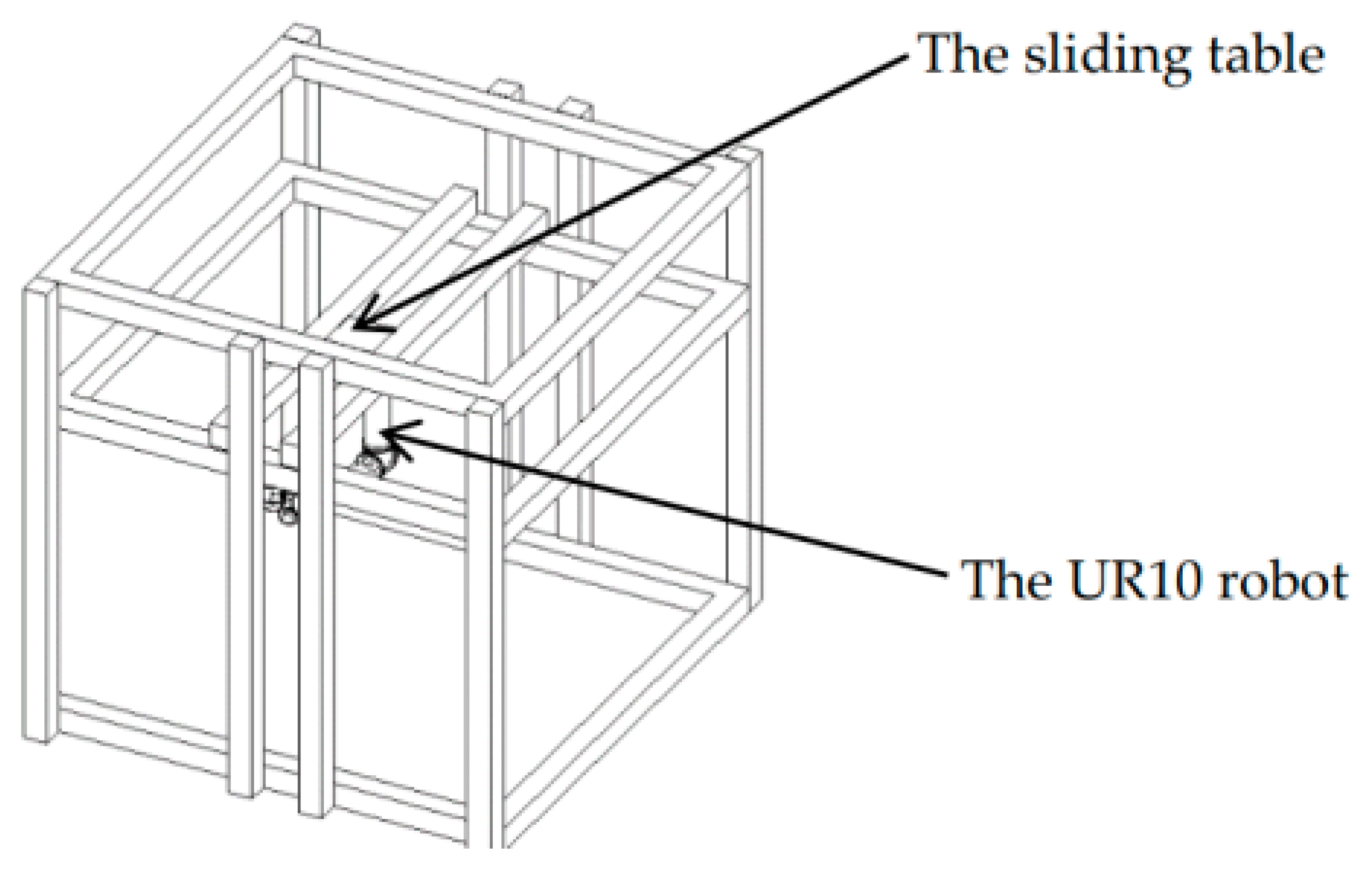
Since the standard 3-dimensional Cartesian coordinate system is chosen as the coordinate system for the base of the UR10 robot, which is shown in Figure 1. The UR10 robot can be installed in upright or upside-down modes on a sliding table. The difference between the two installation modes lies in whether the robot is upright or upside down relative to the sliding table. When a larger workpiece is to be processed by the UR10 robot, the UR10 robot is installed upside down and is not in the same direction as the z-axis of the standard 3-dimensional Cartesian coordinate system. When a small workpiece is to be processed by the UR10 robot, the UR10 robot is installed upright. This paper studies the upside-down installation as are shown in Figure 2.

3. The Kinematics Model of the UR10 Robot

If the origin in the standard 3-dimensional Cartesian coordinate system for the UR10 robot system is the same as the origin of the 3-dimensional coordinate system for the sliding table, the x-, y-, and z-axes of both are the same. Equation (1) describes the pose of the end robot. In Equation (1), Tdis, Ttool, and Trobot, which are all relative poses, represent the pose of the end of the laser focus relative to the origin of the laser, the pose of the origin of the laser relative to the origin of the UR10 robot, and the pose of the end actuator relative to its installation center. Equation (2) indicates the Trans moving operator and Equation (3) indicates Rot(x, θ) rotation operator.
T = T r a n s t x , t y , t z R o t x , θ T robot T tool T dis
T r a n s t x , t y , t z = 1 0 0 t x 0 1 0 t y 0 0 1 t z 0 0 0 1
R o t x , θ = 1 0 0 0 0 cos θ sin θ 0 0 sin θ cos θ 0 0 0 0 1
In Equation (1), only the sliding table and the UR10 robot can move in the entire UR10 robot system. Then, the two can be analyzed separately. As the structure and kinematic model of the sliding table are very easy to analyze, this paper only discusses the kinematic model of the robot.

4. The Forward Kinematics Analysis

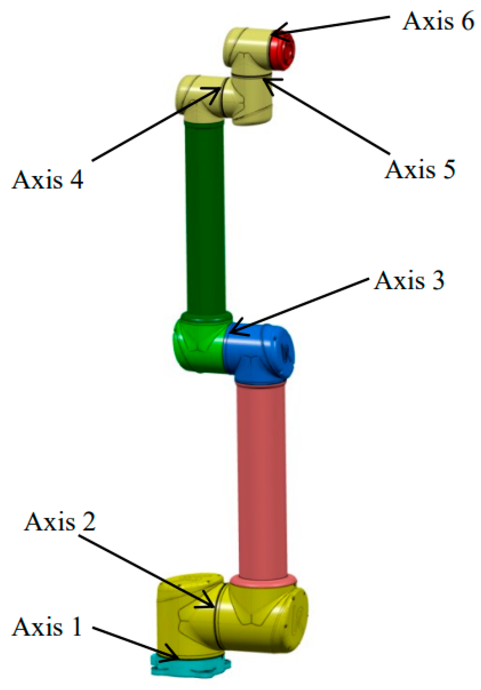
The six rotating joints, which are shown in Figure 3, can be found in the structural diagram of UR10 which is shown in Figure 4, where the pose of the tail end of each joint is represented by one of the six numbers 1 to 6, and 0 represents the position of the origin of the standard 3-dimensional Cartesian coordinate system on the base of the robot.
For the pose change from the coordinates of the UR robot’s base to the end effector, the pose change matrix T i i 1 between adjacent joints can be obtained through the DH model, as is shown in Equation (4).
T i i 1 = R o t z , θ i T r a n s 0 , 0 , d i T r a n s a i , 0 , 0 R o t x , α i
The expression Rot(z, θ) is shown in Equation (5).
R o t z , θ = cos θ sin θ 0 0 sin θ cos θ 0 0 0 0 1 0 0 0 0 1
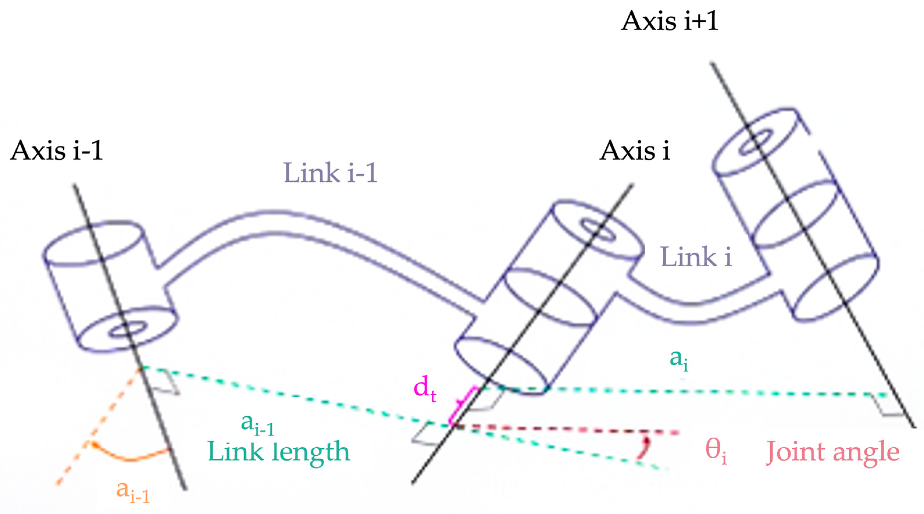
In Equation (4), θi is the angle for which xi−1 spins around zi to become xi; di is the distance between xi−1 and xi along zi; ai is the distance between zi and zi+1 along xi, and αi is the angle for which zi spins around xi to become zi+1. Rot(z, θi) represents the rotation matrix of the z-axis; θi, di, αi, and ai are shown in Figure 5.
Equations (2), (3), and (5) are introduced into Equation (4) to obtain Equation (6), where c represents the cosine function and s represents the sine function.
T i i 1 = c θ i s θ i c α i s θ i s α i a i c θ i s θ i c θ i c α i c θ i s α i a i s θ i 0 s α i c α i d i 0 0 0 1
Successive multiplication is conducted on T i i 1 . Then, the end effector’s transformation matrix, which is shown in Equation (7), relative to the base of the UR10 robot can be obtained.
T robot = i = 1 6 T i i 1
Equations (6) and (7) are utilized to establish the transformation matrix of the UR10 robot’s forward kinematics model.

5. Inverse Kinematics Analysis

There are two methods to resolve inverse kinematics. One is the numerical solution and the other is the analytical solution. The numerical solution model employs the iterative algorithm to find the optimal solution that meets the requirements. In this research, the SQP and BP-SQP algorithms are harnessed to establish the numerical solution model. The analytical solution is to establish an equation set through the spatial structure of each joint of the UR10 robot to obtain the inverse kinematics model of the UR10 robot.

5.1. The Closed-Form Solution of Inverse Kinematics

According to Figure 2, the joint axes represented by 2, 3, and 4 in Figure 2 are parallel. According to Pieper criteria, the closed-form solution is utilized to obtain the sequence of the UR10 Robot’s joint angles under the constraint of the target pose.
The closed-form solution is employed to first establish Equation (8) according to Equation (7) and then establish Equation (9) via Equation (8).
T 1 0 1 T robot = i = 2 6 T i i 1
c θ 6 s θ 5 s θ 6 s θ 5 c θ 5 d 2 + d 3 + d 4 + d 6 c θ 5 + a 5 s θ 5 + a 6 c θ 6 s θ 5 T = n y c θ 1 + n x s θ 1 o y c θ 1 + o x s θ 1 a y c θ 1 + a x s θ 1 y c θ 1 + x s θ 1 T
Because d 2 = d 3 = a 5 = a 6 = 0 , Equation (9) is expanded to obtain Equation (10). The radian value of joint 1, θ 1 , can be obtained via Equation (10). According to the range of motion of joint 1, four solutions can be obtained in for θ 1 in Equation (10).
c d 4 + d 6 a y c θ 1 + d 6 a x s θ 1 = y c θ 1 + x s θ 1 d 4 = y d 6 a y 2 + x d 6 a x 2 sin θ 1 + , tan = y d 6 a y x d 6 a x
Through the radian value of the first joint θ 1 , the radian value of the joint 5, θ 5 , and the radian value of the joint 6 θ 6 . After Equation (11) is resolved, according to the range of motion of joint 5, four solutions can be obtained for θ 5 , two solutions can be obtained for θ 6 .
θ 5 θ 6 = a cos a y c θ 1 + a x s θ 1 a tan 2 n y c θ 1 + n x s θ 1 , o y c θ 1 + o x s θ 1
To obtain θ 2 , θ 3 , and θ 4 , θ 1 , θ 5 , and θ 6 are utilized. With Equation (12), an equation for θ 2 , θ 3 , and θ 4 , Equation (12) is expanded to obtain Equation (13), where θ i 1 i 2 i n = j = 1 n θ i j .
L = T 1 0 1 T 6 0 T 5 4 1 T 6 5 1 = i = 2 4 T i i 1 = R
R = c θ 234 0 s θ 234 a 3 c θ 23 + a 2 c θ 2 s θ 234 0 c θ 234 a 3 s θ 23 a 2 c θ 2 0 1 0 d 4 0 0 0 1
Equation (14) provides the solution for θ 2 , θ 3 , and θ 4 . Therefore, θ234 has two solutions. Both θ 23 and θ 2 have four solutions. In Equations (9), (11), and (13), c represents the cosine function and s represents the sine function.
θ 234 θ 23 θ 2 θ 3 θ 4 = a tan 2 L 21 , L 11 a cos L 14 + L 24 2 a 3 π 4 a cos L 14 a 3 c θ 23 a 2 θ 23 θ 2 θ 234 θ 23
According to the above-mentioned method, there are 1024 closed-form solutions for each pose and hence the initial radian solution of the Euler solution with the least distance needs to be selected.

5.2. The SQP Algorithm for Inverse Kinematics

The SQP algorithm is an iterative algorithm, whose principle is that within the allowed inaccuracy the constraint condition is the total amount of rotation radians of the industrial robot’s joints are the minimum when the industrial robot reaches the target attitude. With this principle, the SQP algorithm establishes the inverse kinematics model of the robot.
The objective function, which is to minimize the sum of the total rotation radians of the joints of the UR10 robot, is built. Equation (15) is the objective function,
f = i = 1 i = 6 θ i r θ i 2
where θ i r and θi are the actual joint radian and starting point radian of the UR10 robot at the target point.
When an iterative algorithm is utilized to resolve the inverse kinematic model of the UR10 robot, due to the existence of Ttool and Tdis, which causes inaccuracy of the end effector to increase. Therefore, the constraint condition of the SQP algorithm can be set as the inaccuracy of the pose of the laser focus. Since the allowed position inaccuracy and pose inaccuracy of the laser focus differ, the position and axial constraints are described in Equations (16) and (17), respectively.
st : j = 1 j = 3 T 6 0 j 4 T 6 0 j 4 2 es 0
n n cos e s
In Equation (16), es′ is the maximal allowable pose inaccuracy, T′ represents the actual pose of the target point, and Tij is the element on the i-th row and j-th column. In Equation (17), n′, equals ( T 0 6 13 , T 0 6 23 , T 0 6 33 ), represents the axis of the laser focus and n represents the actual axial direction of the target points.
The SQP algorithm decomposes a problem into QP (quadratic programming) sub-questions. By finding the descending direction d of the current angle sequence θk in QP sub-questions and updating θk+1 via d, the SQP algorithm meets the Karush–Kuhn–Tucker (KKT) conditions or reaches the maximum number of iterations. The precise operation process of the SQP algorithm is described below.
In the first step, the current Lagrangian function L(θk, λ) which is depicted in Equation (18), of the current angle sequence θk is established.
L θ k , λ = f θ k + λ g θ k
In equation (18), λ, which is larger than 0, is the Lagrange multiplier.
In the second step, the descending direction d of the current θk is identified. Equation (18) can be transformed into the solution for d, which is shown in Equation (19). The Hessian matrix in L(θk, λ) is represented by Hk.
min d f θ k T d + d T H k d 2 s t : g θ k + g θ k T d 0
In the third step, the angel sequence is updated and θk+1 equals θk plus d. Whether the result meets the KKT conditions or reaches the maximum number of iterations is determined. If the result meets the KKT conditions or reaches the maximum number of iterations, iterations will be terminated. If not, the second step is repeated. Equation (20) shows the KKT conditions.
f θ k + λ g θ k = 0 ; λ 0 ; g θ k 0 ; λ g θ k = 0
In the KKT conditions, the third condition means that result satisfies the constraint condition, where if g(θk) equals 0, the KKT condition becomes ▽f(θk) which equals 0, and the derivative of the point with a minimal value is 0, and if g(θk) is smaller than 0, λ equals 0 and the KKT condition becomes ▽f(θk) which equals 0.

5.3. The Solution of the Inverse Kinematics Model with the BP-SQP Algorithm

According to the characteristics of the SQP algorithm, the SQP algorithm depends on the initial values greatly, and deviations will happen. The initial value of the SQP algorithm is optimized by the BP neural network to reduce the errors caused by dependence on the initial values.
The BP neural network uses forward propagation for its output results and backpropagation for its errors. Therefore, it is not necessary to clarify the equation of the relationship between the output value and the input value in advance. The BP neural network only needs to complete its own training and rules to obtain the optimal output value after the input value is imported. The BP neural network is based on the back-propagation errors to achieve the training of the multi-front layer network and based on the gradient descent method to achieve the minimum mean square error between the expected and actual output. In the BP neural network, the number of layers, the adjacent combination form, and the number of nodes contained in each layer must be known in advance. Only by confirming the number of layers of the neural network and the number of nodes in each layer, the actual network structure can be confirmed.
To simulate any continuous function, only a three-layer neural network is needed. According to the above analysis, the inverse kinematics model of the UR10 robot can be decomposed into several continuous and complex functions. When a continuous trajectory, which the same function is selected to represent, is executed by the UR10 robot, the three-layer neural network can be used to solve the inverse kinematics of the UR10 robot’s trajectory. In this paper, a 3-layer BP neural network is employed to simulate the inverse kinematics of the UR10 robot. The three layers refer to the input layer, hidden layer, and output layer.
The number of nodes in the input layer is the number of input independent variables. The input is the pose of the target point which includes the target point’s pose matrix R and the position, x, y, and z coordinates. As the Euler angle leads to the problem of the UR10 robot’s joints being locked, four elements are introduced to describe to target point’s pose matrix. Equations (21) and (22) demonstrate the transformation between the rotation matrix R of the target point and the four elements q0, q1, q2, q3. Therefore, the number of nodes in the input layer of The BP neural network employed in this paper is seven.
q 3 q 2 q 1 q 0 = 1 + R 11 2 + R 22 2 + R 33 2 / 2 R 21 R 12 / 4 q 3 R 13 R 31 / 4 q 3 R 32 R 23 / 4 q 3
R = 1 2 q 1 2 2 q 2 2 2 q 0 q 1 2 q 2 q 3 2 q 0 q 2 + 2 q 1 q 3 2 q 0 q 1 + 2 q 2 q 3 1 2 q 0 2 2 q 2 2 2 q 1 q 2 2 q 0 q 4 2 q 1 q 2 2 q 1 q 3 2 q 1 q 2 + 2 q 0 q 3 1 2 q 0 2 2 q 1 2
Since there is a large difference in orders of magnitude between X, Y, Z, and q0, q1, q2, q3, Z-score, which is a standardization equation, is used to convert all input values into the same order of magnitude. Equation (23) represents the Z-score equation.
x = x μ σ
In Equation (23), μ represents the mean value of the samples and σ represents the standard deviation.
The number of nodes on the output layer is the number of dependent variables of the 3-layer BP network, whose output values are the six joint radians, θ1, θ2, θ3, θ4, θ5, and θ6. The number of nodes on the output layer of the 3-layer BP network is six.
The number of nodes on the hidden layer of the BP neural network, which is often decided by the equations created by previous researchers, is undetermined. Equation (24), which is invented by previous researchers, is utilized to determine the number of nodes on the hidden layer.
m = n + l + a
In Equation (24), m represents the number of nodes on the hidden layer, n represents the number of nodes on the input layer, l represents the number of nodes on the output layer, and a is a constant between two and ten. According to the BP neural models created by previous researchers, a is given the value of 2. Therefore, the number of nodes on the hidden layer is six.

5.3.1. Forward Propagation of Neural Networks

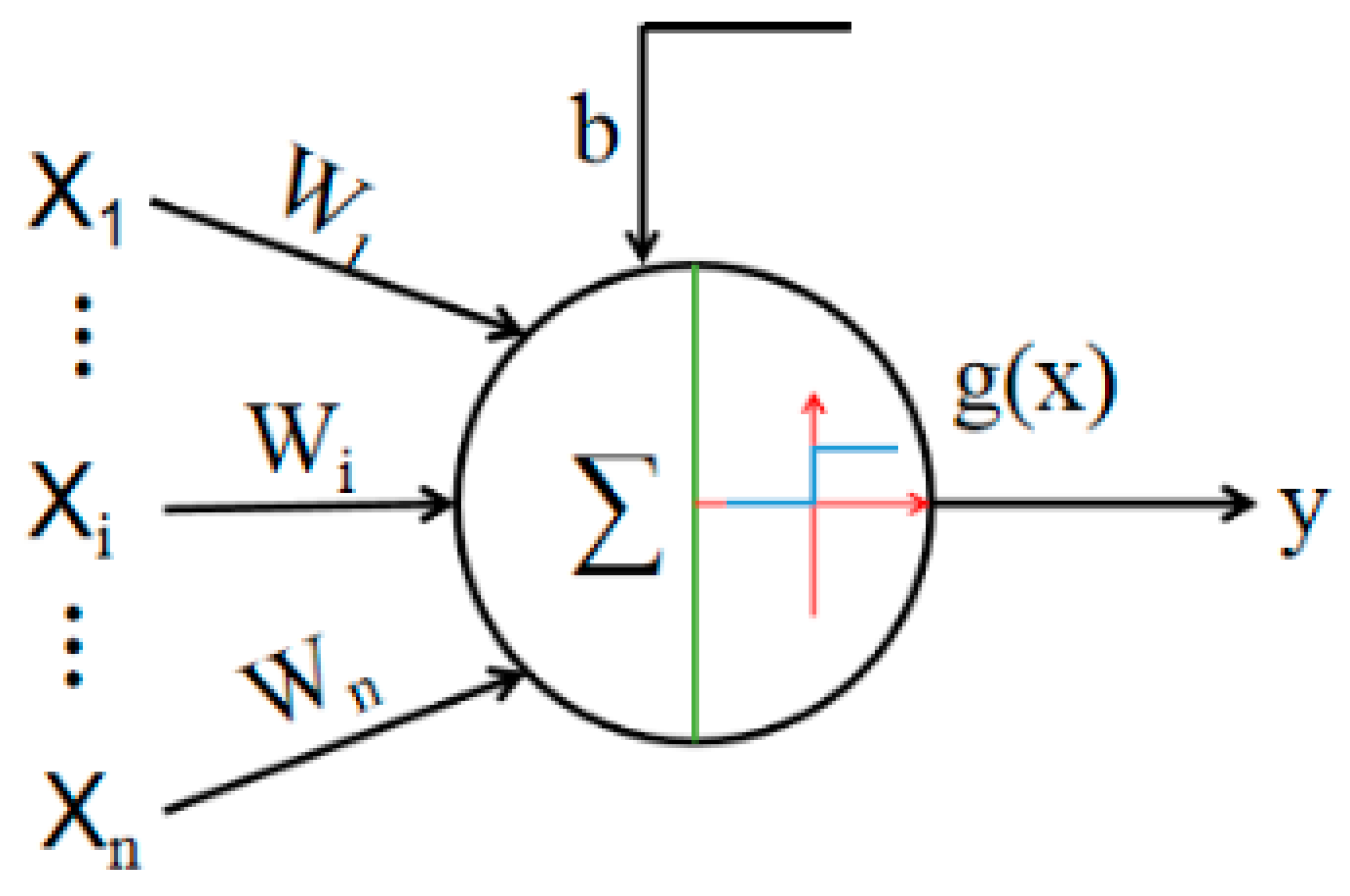
The forward propagation of neural networks refers to finding the true output value according to the input layer. Figure 6 shows the output model of each neuron.
If the nonlinearity needs to be improved, activation functions should be considered. The frequently used functions are the ReLu function and tanh function. As per the comparison of the two functions, the convergence rate of the tanh function is ideal and its gradient changes greatly. Therefore, the tanh function is selected as the activation function of the BP neural network. Equation (25) describes the tanh function.
tan h x = e x e x e x + e x

5.3.2. Back Propagation of Neural Networks

The backpropagation of neural networks is to change the values of w, which represents weights, and b, which represents biases, in neurons according to the difference between the actual and expected output values. Adding a loss function to the network helps express the difference between the expected value and the actual value in the forward propagation. There is a positive correlation between accuracy and loss function. In order to facilitate the research, the samples’ error squared and half the selected equation is chosen as the loss function of the neural network, and the mean square deviation of the samples is shown in Equation (26).
L w 0 i j , w 1 j , b 0 i , b 1 = 1 2 k = 1 N j = 1 6 y j k y j k 2 = 1 2 k = 1 N r k 2
In Equation (26), Y j k represents the output value of the j-th theory of the k-th sample and Y j k is the j-th actual output value of the k-th sample, and rk is the loss value of the k-th sample.
Among the commonly used neural network algorithms, the LM algorithm is more appropriate and is therefore selected. Equation (27) is the updating model of w and b, J is the Jacobian matrix of the loss function, λ represents the penalty factor, and xk represents the value of w and b iterated to the k-th time. In Equation (27), λ_inc and λ_dec represent the increment and decrement of λ, respectively.
x k + 1 = x k J T J + λ I 1 J T r
λ = λ λ _ inc : J T   and   J   are   non   positive   definite λ λ _ dec : The   loss   function - value   increases
J = r 1 x 1 r 1 x 2 r 1 x m r 2 x 1 r 2 x 2 r 2 x m r N x 1 r N x 2 r N x m
According to Equations (27)–(29), to obtain the updated values of w and b at each time of iteration, only r k r w needs to be resolved. The derivative of the activation function is shown in Equation (30). The partial derivatives induced by w i j 1 and b i 1 on the output layer are shown in Equation (31), where Y i k and Z i k represent the actual output value of the i-th node on the output layer or hidden layer measured at the k-th time. Forward propagation of the neural network can be utilized to obtain the values of Y i k and Z i k .
x k + 1 = x k J T J + λ I 1 J T r
λ = λ λ _ inc : J T   and   J   are   non   positive   definite λ λ _ dec : The   loss   function - value   increases
The equation that updates the w and b of the hidden layer is shown in Equation (32),
r k w 0 i j = c = 1 6 r k Y c k Y c k w 0 i j = c = 1 6 r k Y c k Y c k a c 1 a c 1 Z i k Z i k a i 0 a i 0 w 0 i j = c = 1 6 r k Y c k 1 Y c k 2 w 1 c i 1 Z i k 2 X j k r k b 0 j = c = 1 6 r k Y c k Y c k w 0 j = c = 1 6 r k Y c k Y c k a c 1 a c 1 Z i k Z i k a i 0 a i 0 w 0 i j = c = 1 6 r k Y c k 1 Y c k 2 w 1 c i 1 Z i k 2
where X j k represents the j-th input value of the k-th sample.
Equations (26) to (32) describe the whole process of backpropagation. When the loss function of the entire neural network is less than the allowed precision or the neural network reaches the maximal number of training, backpropagation of the neural network is terminated.

6. Simulation Based on Inverse Kinematics

One of the tracks was randomly selected for the simulation experiment, and the three algorithms mentioned above were used in turn to set the evaluation criteria as the position allowable error and axis allowable error.
When the closed-form solution was used, the Rodrigues rotation formula was utilized to obtain one of the possible poses of the target point, and Trobot, which equals T∙(TtoolTdis)−1 is taken as the actual pose of the UR10 robot’s end effector. Equation (33) describes the Rodriguez formula, Where n0 equals [0,0,1]T, and r is the vector product of n and n0.
R = E cos θ + 1 cos θ r T r + sin θ 0 r z r y r z 0 r x r y r x 0
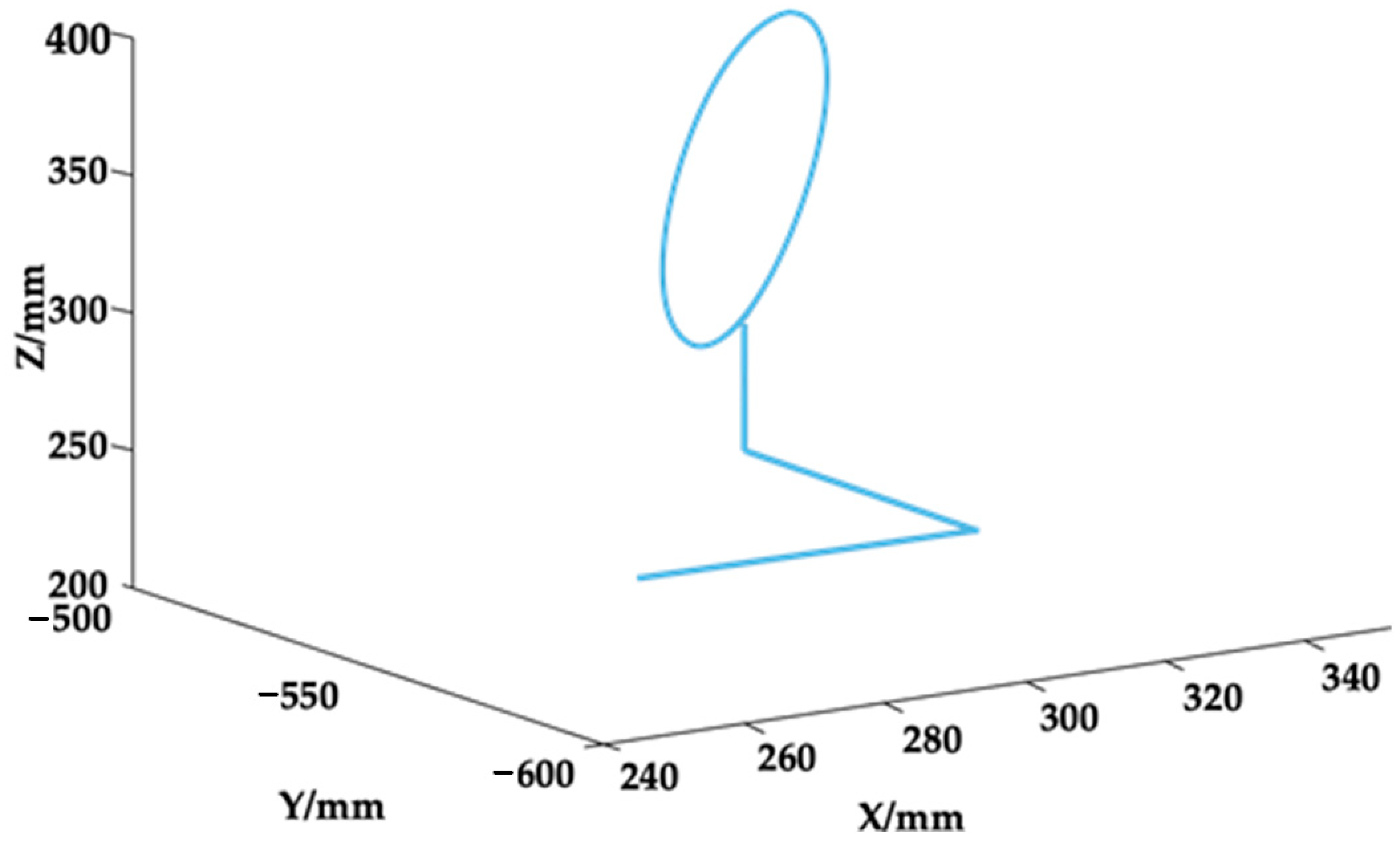
In the BP-SQP and SQP algorithms, the permitted error value for the position is usually set to 0.01–0.03 mm, according to engineering experience, we take the maximum of 0.03 mm here. Likewise, for the axis set to 0.11°. The selected track includes 500 points, and the selection step was set to 0.6 mm. Figure 7 is the trajectory diagram.
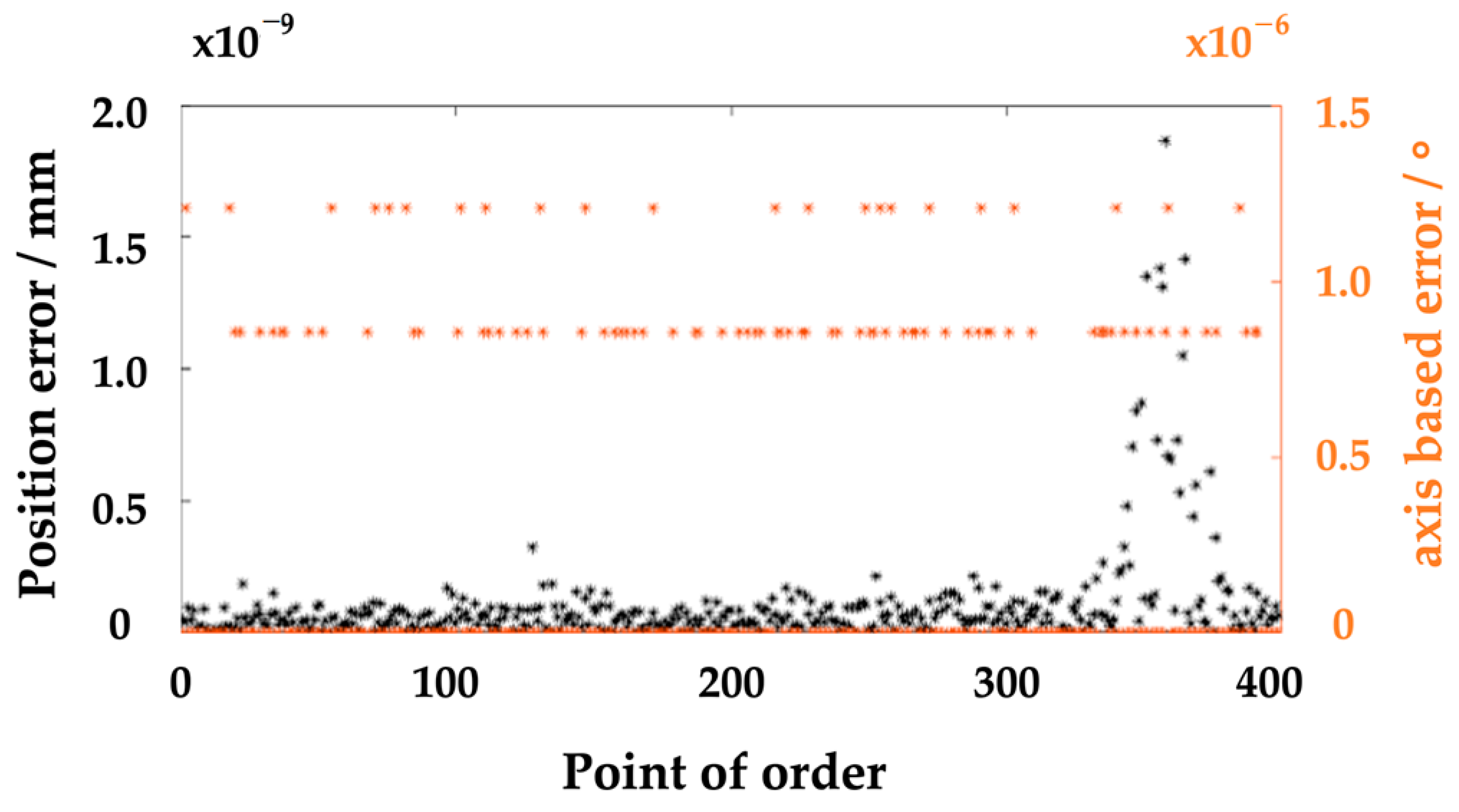
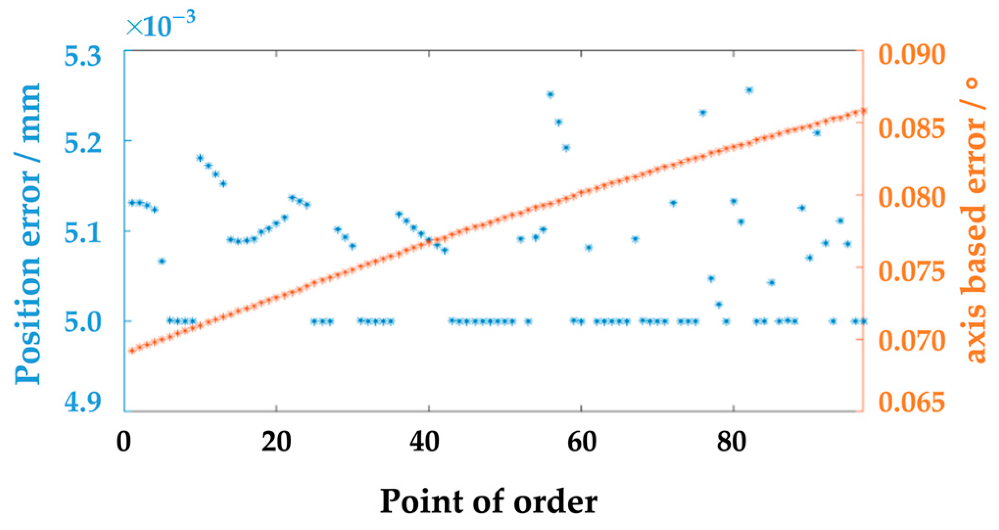
The target trajectory was analyzed with the closed-form solution. The accuracy was 100%. The position and axis-based errors of all points were recorded. The result is shown in Figure 8. The observation showed that both errors were far lower than the allowable errors. Then, inverse kinematics obtained by this the closed-form solution can be regarded as the real inverse kinematic solution. The total time taken to find the solution was 78.8 s.
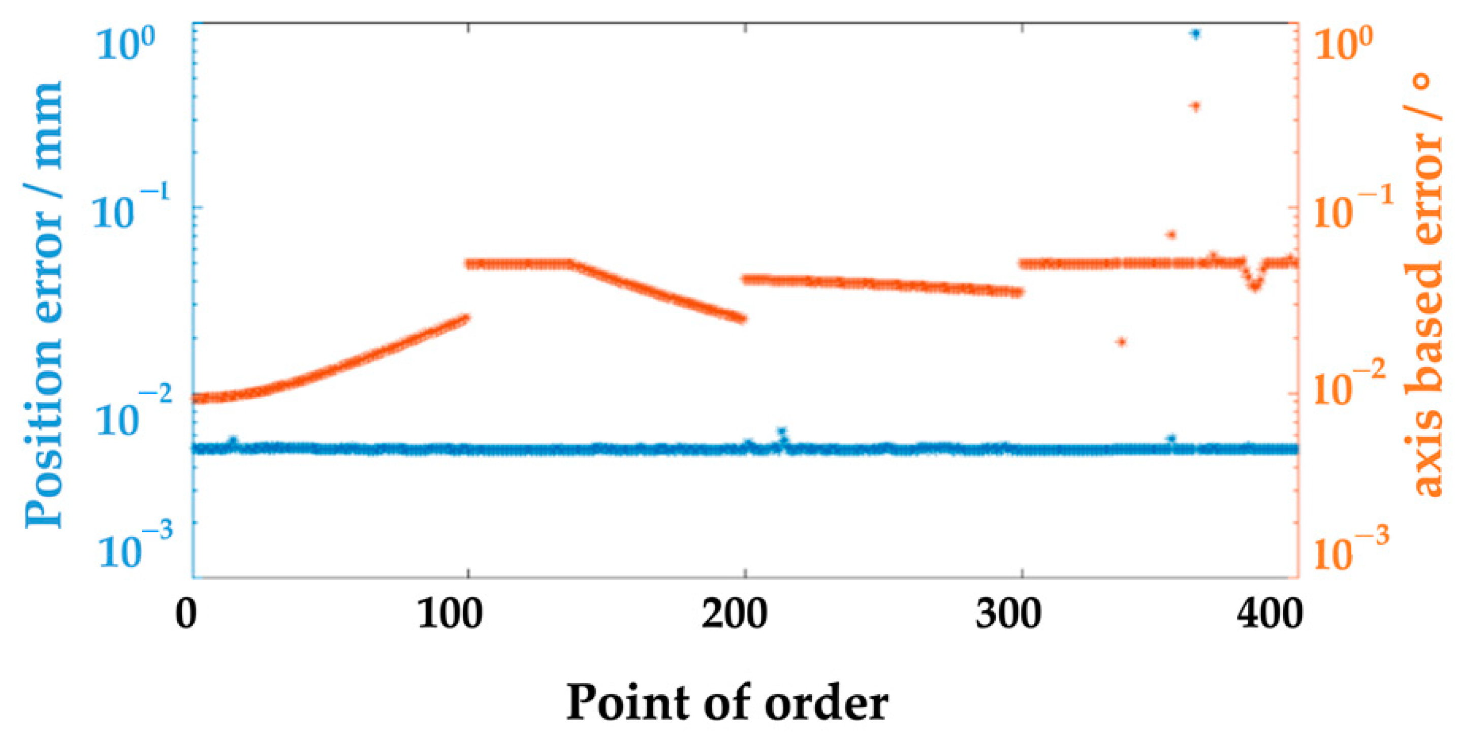
The initial value of the SQP algorithm was set as the joint angle value of the previous point of the closed-form solution, and half of the position and axis based errors were introduced into Equation (2). The results are shown in Figure 9, according to which most of the points from the UR10 robot’s kinematics via the SQP algorithm meet the kinematic accuracy requirements, and only two are outside the allowed range. The accuracy of the SQP algorithm is 99.5%. The total time taken for the SQP algorithm to find the solution was about 37 s, which is less than half of the time taken by the closed-form solution.
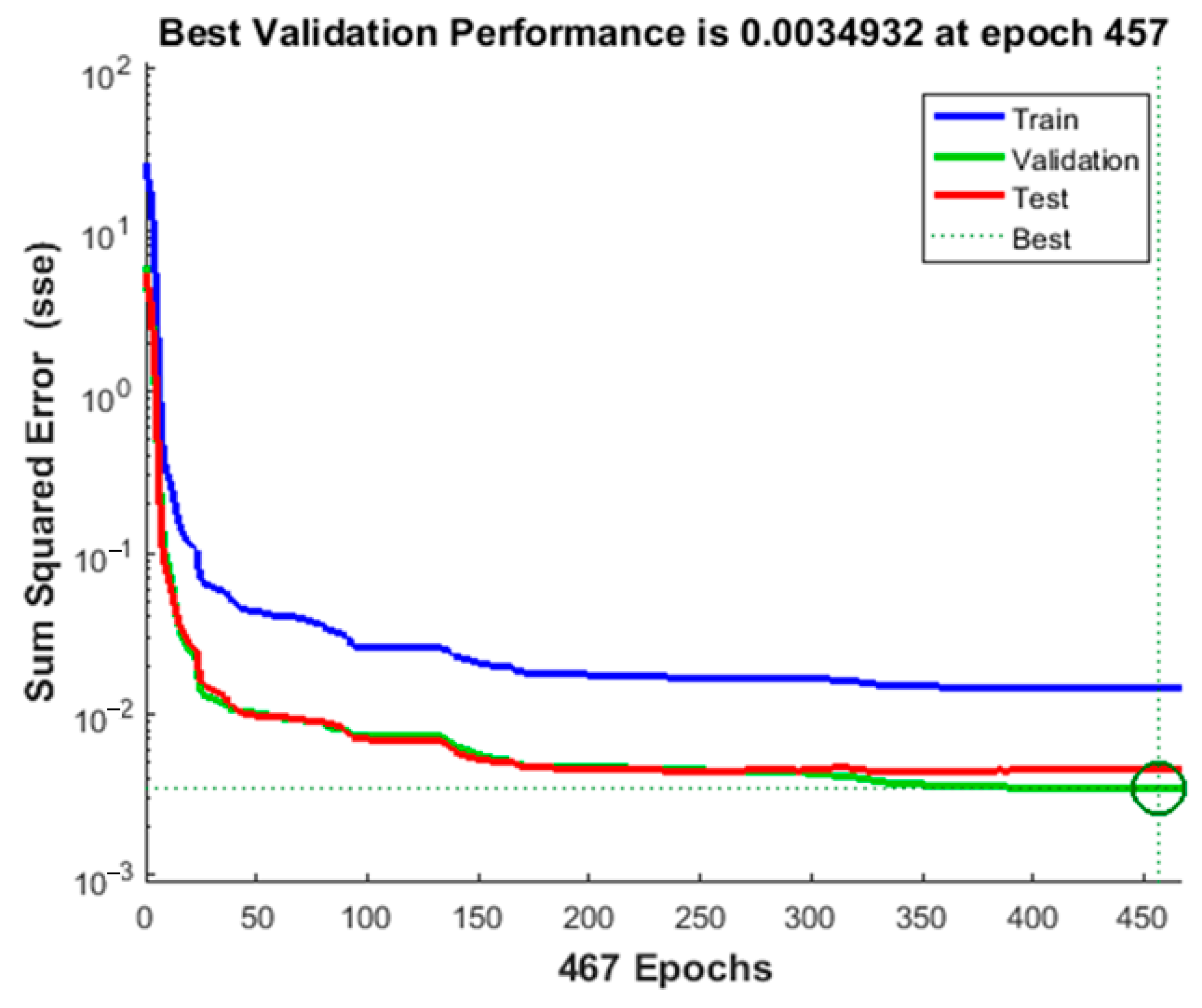
When the BP neural network was utilized, the top 400 points which met the accuracy requirement in the SQP algorithm were extracted as the training set, and the remaining 98 points were extracted as the prediction set. In the P neural network of the simulation experiment, λ equaled 0.001, λ_inc equaled 10, and λ_dec equaled 0.1, which were the default initial values of the LM algorithm. The highest number of failed iterations was 10. The total time taken by the BP-SQP algorithm to resolve the UR10 robot’s inverse kinematic was 13.1 s. The simulation results are shown in Figure 10, according to which the BP neural network during the training process divided tested samples into three sets, the training set, the verification set, which is the data set of the BP neural network’s initial verification model, and testing set, which is the data set that tested the fitting result of the BP neural network. The accuracy of the BP neural network’s testing set and verification set was 0.003. The accuracy of the BP neural network’s training set was 0.002 and met the actual requirement. The data from the training set was input into the BP neural network. The output values obtained from the neural network were chosen as the initial value of SQP. Figure 11 shows the experimental results of the BP-SQP algorithm. The time taken by the BP-SQP algorithm to resolve the UR10 robot’s inverse kinematics was only 4.2 s. The success rate of the simulation reached 100%. The results obtained from the three methods are shown in Table 1.
From the results in Table 1, both the closed-form solution method and the BP-SQP algorithm are 100% accurate, and the SQP algorithm is slightly less accurate at 99.5%. In terms of running time, the closed-form solution method takes the most time (78.8 s), and the SQP takes nearly half the time of the closed-form solution method (37 s). The BP-SQP algorithm takes the least time (4.2 s) and can get the optimal solution as well as the SQP algorithm, but there is a requirement that a certain number of samples be used.
Considering the advantages and disadvantages of the three algorithms, the closed-form solution method can be used when it is used for the first time and the correct rate is required, and the SQP algorithm is used when it is used for the first time and the speed is required. When a certain number of samples are collected the BP-SQP algorithm can improve the correct rate and speed. They can be flexibly selected according to the actual working conditions and used with each other to better meet the requirements under the real working conditions.

7. Conclusions

The inverse kinematic model of the UR10 robot based on the SQP algorithm and BP-SQP algorithm is studied. For the SQP algorithm is too dependent on the initial value, which is easy to produce deviation and affects the solution speed and accuracy of the algorithm, we use BP neural network to optimize the initial value, propose the BP-SQP algorithm, and add the closed solution method to analyze and compare these three algorithms. The results show that the algorithm accuracy of the closed-form solution of inverse kinematics was 100% but the closed-form solution took too much time to resolve the UR10 robot’s inverse kinematics. The pose of the target subject needed to be determined and the solution to inverse kinematics by the closed-form method was not the optimal solution. Although the accuracy of the SQP algorithm was not 100%, the time consumed by the SQP algorithm was only half the time taken by the closed-form method, and the optimal solution was obtained. Although The SQP algorithm optimized by the BP neural network needed stringent preconditions for its operation, it took the least time to obtain the solution, which was the optimal solution, under the condition of 100% accuracy.

Author Contributions

Conceptualization, Y.H. and J.W.; methodology, Y.H. and J.W.; software, J.L.; validation, J.L., X.Z. and X.L.; formal analysis, X.Z.; investigation, X.L.; resources, Q.H.; data curation, X.T.; writing—original draft preparation, Y.H. and X.T.; writing—review and editing, J.W. and S.C.; visualization, C.W.; supervision, S.C.; project administration, C.W. and Q.H. All authors have read and agreed to the published version of the manuscript.

Funding

This research was funded by the National Natural Science Foundation of China, grant number 52005169.

Institutional Review Board Statement

Not applicable.

Informed Consent Statement

Not applicable.

Data Availability Statement

Not applicable.

Conflicts of Interest

The authors declare no conflict of interest.

References

  1. Moreira, A.P.; Neto, P.; Vidal, F. Special Issue on Advances in Industrial Robotics and Intelligent Systems. Appl. Sci. 2023, 13, 1352. [Google Scholar] [CrossRef]
  2. Xiao, Y.; Jiang, J.; Yang, D.; Li, J.; Wu, J.; Chen, Y. Research on Mechanism and Measurement Model for the Effects of Path Dependence on Human Error in Space Station Manipulator Tasks. Symmetry 2022, 14, 753. [Google Scholar] [CrossRef]
  3. Kampmann, P.; Kirchner, F. Integration of Fiber-Optic Sensor Arrays into a Multi-Modal Tactile Sensor Processing System for Robotic End-Effectors. Sensors 2014, 14, 6854–6876. [Google Scholar] [CrossRef]
  4. Guerra, E.; Munguia, R.; Grau, A. Monocular SLAM for Autonomous Robots with Enhanced Features Initialization. Sensors 2014, 14, 6317–6337. [Google Scholar] [CrossRef] [Green Version]
  5. Chang, C.; Han, Z.; Li, X.; Sun, S.; Qin, J.; Fu, H. A Non-Geodesic Trajectory Design Method and Its Post-Processing for Robotic Filament Winding of Composite Tee Pipes. Materials 2021, 14, 847. [Google Scholar] [CrossRef]
  6. Wang, J.; Liang, F.; Zhou, H.; Yang, M.; Wang, Q. Analysis of Position, Pose and Force Decoupling Characteristics of a 4-UPS/1-RPS Parallel Grinding Robot. Symmetry 2022, 14, 825. [Google Scholar] [CrossRef]
  7. Huang, H.; Xu, H.; Chen, F.; Zhang, C.; Mohammadzadeh, A. An Applied Type-3 Fuzzy Logic System: Practical Matlab Simulink and M-Files for Robotic, Control, and Modeling Applications. Symmetry 2023, 15, 475. [Google Scholar] [CrossRef]
  8. Tatum, R.; Lucas, D.; Weaver, J.; Perkins, J. Geometrically motivatied inverse kinematics for an arm with 7 degrees of freedom. In Proceedings of the OCEANS 2015-MTS/IEEE WASHINGTON, Washington, DC, USA, 19–22 October 2015; pp. 1–6. [Google Scholar]
  9. Liu, H.S.; Zhou, W.N.; Lai, X.B.; Zhu, S. An Efficent Inverse Kinematic Algorithm for a PUMA560-Structured Robot Manipulator. Int. J. Adv. Robot. Syst. 2013, 10, 236. [Google Scholar] [CrossRef]
  10. Bai, Y.; Luo, M.; Pang, F. An Algorithm for Solving Robot Inverse Kinematics Based on FOA Optimized BP Neural Network. Appl. Sci. 2021, 11, 7129. [Google Scholar] [CrossRef]
  11. Kramar, V.; Kramar, O.; Kabanov, A. An Artificial Neural Network Approach for Solving Inverse Kinematics Problem for an Anthropomorphic Manipulator of Robot SAR-401. Machines 2022, 10, 241. [Google Scholar] [CrossRef]
  12. Siciliano, B.; Khatib, O. Springer Handbook of Robotics; Springer: Berlin/Heidelberg, Germany, 2008; pp. 84–85. [Google Scholar]
  13. Zhao, G.; Jiang, D.; Liu, X.; Tong, X.; Sun, Y.; Tao, B.; Kong, J.; Yun, J.; Liu, Y.; Fang, Z. A Tandem Robotic Arm Inverse Kinematic Solution Based on an Improved Particle Swarm Algorithm. Front. Bioeng. Biotechnol. 2022, 10, 832829. [Google Scholar] [CrossRef] [PubMed]
  14. Duka, A.-V. Neural Network based Inverse Kinematics Solution for Trajectory Tracking of a Robotic Arm. Procedia Technol. 2014, 12, 20–27. [Google Scholar] [CrossRef] [Green Version]
  15. Gan, J.Q.; Oyama, E.; Rosales, E.M.; Hu, H. Quick look a complete analytical solution to the inverse kinematics of the pioneer 2 robotic arm. Robotica 2005, 23, 123–129. [Google Scholar] [CrossRef]
  16. Sudharsan, J.; Karunamoorthy, L. Derivation of Forward and Inverse Kinematics of 8—Degrees of Freedom Based Bio-Inspired Humanoid Robotic Arm. Adv. Mater. Res. 2014, 984–985, 1245–1252. [Google Scholar] [CrossRef]
  17. Deng, H.; Xie, C. An improved particle swarm optimization algorithm for inverse kinematics solution of multi-DOF serial robotic manipulators. Soft Comput. 2021, 25, 13695–13708. [Google Scholar] [CrossRef]
  18. Liu, S.; Zhu, S.; Wang, X. Real-time high-precision inverse kinematics algorithm for general 6R robots based on matrix decomposition. J. Mech. Eng. 2008, 44, 304–309. [Google Scholar] [CrossRef]
  19. Lü, S.; Zhang, D.; Liu, H. The inverse kinematics spinor equation of 6R robot based on Wu method. J. Mech. Eng. 2010, 46, 35–41. [Google Scholar]
  20. Liao, B.; Shang, J.; Ernest, A.; Wang, X. Five degree of freedom inverse kinematics of anthropomorphic arm based on ergodic iteration method. Mech. Des. Res. 2011, 27, 25–28. [Google Scholar]
  21. Si, Y.; Jia, Q.; Chen, G.; Sun, H. A complete solution to the inverse kinematics problem for 4-DOF manipulator robot. In Proceedings of the 2013 IEEE 8th Conference on Industrial Electronics and Applications (ICIEA), Melbourne, VIC, Australia, 19–21 June 2013; pp. 1880–1884. [Google Scholar] [CrossRef]
  22. Lin, Y.; Min, H. Inverse kinematics of modular manipulator robot with shoulder offset based on geometric method mixed with analytical method algorithm. In Proceedings of the 2015 IEEE International Conference on Cyber Technology in Automation, Control, and Intelligent Systems (CYBER), Shenyang, China, 8–12 June 2015; pp. 1198–1203. [Google Scholar] [CrossRef]
  23. Zhang, J.; Xu, W.; Meng, D. Inverse kinematics solution method of redundant space manipulator based on arm angle parameterization. In Proceedings of the 32nd Chinese Control Conference, Xi’an, China, 26–28 July 2013; pp. 6022–6027. [Google Scholar]
  24. Yu, L.; Wang, W.; Wang, Z.; Gu, Q.; Wang, L. An analytical solution acquisition method for inverse kinematics of robots not satisfying pieper criterion. Robot 2016, 38, 486–494. [Google Scholar]
  25. Li, Q.; Zhao, L.; Li, R.; Liu, R.; Feng, Y.; Zhang, P. Inverse kinematics and workspace analysis of SPR+UPS+UPR parallel mechanism. Packag. Eng. 2020, 41, 213–218. [Google Scholar]
  26. Cui, M.; Wu, J.; Li, R.; Wang, X.; Zhang, J. Inverse kinematics and reachable workspace analysis of 3-URPR parallel mechanism. Packag. Eng. 2020, 41, 196–201. [Google Scholar]
  27. Yang, S. Improved drosophila optimization algorithm for inverse kinematic solutions of redundant robots. Mech. Strength 2020, 42, 7. [Google Scholar]
  28. Xie, X.; Fan, S.; Zhou, X.; Li, Z. Inverse solution of robotic arm kinematics based on improved differential evolutionary algorithm. Robotics 2019, 41, 8. [Google Scholar]
  29. Wang, J.; Yang, M.; Liang, F.; Feng, K.; Zhang, K.; Wang, Q. An Algorithm for Painting Large Objects Based on a Nine-Axis UR5 Robotic Manipulator. Appl. Sci. 2022, 12, 7219. [Google Scholar] [CrossRef]
  30. Kucuk, S.; Bingul, Z. Inverse kinematics solutions for industrial robot manipulators with offset wrists. Appl. Math. Model. 2014, 38, 1983–1999. [Google Scholar] [CrossRef]
  31. Bingül, Z.; Karahan, O. Dynamic identification of Staubli RX-60 robot using PSO and LS methods. Expert Syst. Appl. 2011, 38, 4136–4149. [Google Scholar] [CrossRef]
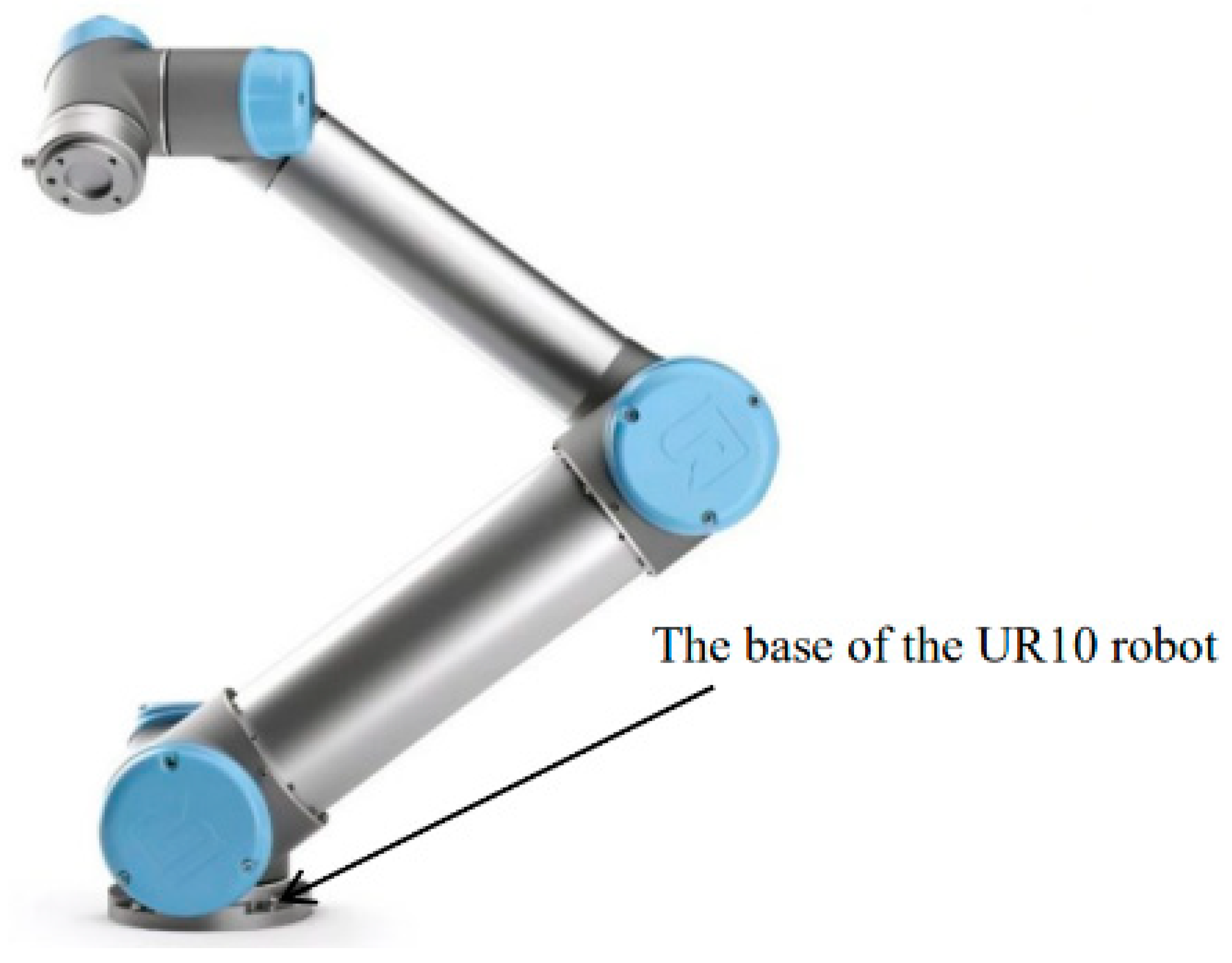
Figure 1. The UR10 robot.
Applsci 13 03009 g001
Figure 2. The upside-down installation of the UR10 robot.
Applsci 13 03009 g002
Figure 3. The six joint axes of the UR10 robot.
Applsci 13 03009 g003
Figure 4. The pose diagram of the UR10 robot.
Applsci 13 03009 g004
Figure 5. The D-H model.
Applsci 13 03009 g005
Figure 6. The output of a neural network.
Applsci 13 03009 g006
Figure 7. The trajectory diagram.
Applsci 13 03009 g007
Figure 8. Inverse kinematics via the closed-form solution.
Applsci 13 03009 g008
Figure 9. The inverse solution via the SQP algorithm.
Applsci 13 03009 g009
Figure 10. Training results of the BP neural network.
Applsci 13 03009 g010
Figure 11. BP-SQP solution of inverse solution.
Applsci 13 03009 g011
Table 1. Comparison of results.
TypeSuccess RateTime/sAlgorithmic PremiseOptimal Solution
The closed-form solution100%78.8Target pose determinationno
The SQP algorithm99.5%37Target position and axis determinationyes
The BP-SQP algorithm100%4.2Target location and axis determination, a certain number of samplesyes
Disclaimer/Publisher’s Note: The statements, opinions and data contained in all publications are solely those of the individual author(s) and contributor(s) and not of MDPI and/or the editor(s). MDPI and/or the editor(s) disclaim responsibility for any injury to people or property resulting from any ideas, methods, instructions or products referred to in the content.