Abstract
For the purpose of fulfilling the low sidelobe level (SLL) requirements for spaceborne phased array antenna pattern synthesis, this paper proposes a new improved whale optimization algorithm (IWOA). As a type of new heuristic algorithm inspired by whale hunting behavior, WOA has the advantages of simple structure, few parameters, fast optimization speed, and high precision. In this paper, improvements are made in three aspects of adaptive weight, spiral coefficient optimization, and optimal neighborhood perturbation, and the proposed algorithm is successfully applied to the intelligent calculation of antenna synthesis. In light of the engineering requirements, the mathematical model of the optimization problem is established, and the desired antenna pattern with high gain and low sidelobe is obtained using IWOA under the constraint that the amplitude variation is within 20 dB. Simulation results demonstrate that IWOA is superior in maximum sidelobe level (MSLL) suppression and convergence. Consequently, EM simulations were conducted on a 64-element planar array, with the results consistent with the theoretical simulation, verifying the feasibility and effectiveness of the proposed algorithm.
1. Introduction
In recent years, the spaceborne array antenna has attracted increasingly extensive attention due to its beamforming, beam steering and high-gain capabilities. For array antenna pattern synthesis, the main concern is to search for the appropriate excitation amplitude and phase to obtain the desired radiation pattern. Various approaches, for example, traditional mathematical techniques and optimization algorithms, have been put forward to the array antenna pattern synthesis problem [1,2,3,4]. Normally, Taylor weighting method and Chebyshev weighting method are commonly used to achieve sidelobe suppression. Nonetheless, the amplitude excitation range satisfying Taylor or Chebyshev distribution is too large to be controlled, leading to the difficulty in its application in practical engineering, whereas the global optimization algorithm can effectively limit the range of amplitude variation. Owing to the limitation of such a device design, in Wilkinson circuit, the signal combination efficiency will be affected when there is a large signal power difference. This study controls the maximum variation range of amplitude to 20 dB in this project. Undoubtedly, if the amplitude change is too small, the sidelobe suppression will be very poor. In practice, this paper has achieved the attenuation control by using attenuators. Low sidelobe level is one of the key technical indicators in the antenna pattern, which can effectively improve the communication quality by facilitating the signal-to-noise ratio, reducing the influence of the clutter signal outside the main beam and enhancing the anti-interference ability of the entire system [5,6,7,8].
Genetic algorithm (GA) and particle swarm optimization (PSO) are the first two popular and classical optimization algorithms, which have been successfully applied to antenna synthesis for their high efficiency and simplicity [9,10,11,12]. However, these two algorithms have the disadvantage of premature convergence in solving multi-parameter optimization problems. Therefore, an increasing number of improved algorithms based on classical GA and PSO have been employed to the antenna synthesis problem [13,14], such as differential evolution algorithm (DE) [15], moth flame optimization algorithm (MFO) [16], fruit-fly optimization algorithm (FOA) [17], invasive weed optimization algorithm (IWO) [18], grey wolf optimization algorithm (GWO) [19], mayfly optimization algorithm (MOA) [20], compressed sensing (CS) [21], biogeography-based optimization (BBO) [22], firefly algorithm (FA) [23], ant colony optimization (ACO) [24], and so on. Despite the fact that these aforementioned algorithms can achieve favorable results in array antenna synthesis, the increase in parameters will lead to slower calculation speed and lower algorithm efficiency. Furthermore, these solutions easily fall into a local optimal solution when the number of phased array elements increases. Therefore, further improvement is needed.
The whale optimization algorithm (WOA) [25] is type of simple but effective swarm optimization algorithm. The research concept originates from the hunting behavior of humpback whales, which was proposed by Australian researchers Seyedali Mirjalili and Andrew Lewis in 2016. WOA has advantages of simple structure and fewer parameters, so it has a faster solving speed and higher precision in the process of solving multivariate functions. In 2018, Zhang applied WOA to the synthesis of wide-sided linear aperiodic arrays with minimum sidelobe level under uniform excitation [26]. It can be clearly seen from these publications that WOA significantly superior to several standard algorithms, both in terms of convergence speed and convergence precision. Therefore, this study investigates the future WOA-based enhancements.
To further improve the global search ability and solution accuracy of the WOA, an improved whale optimization algorithm (IWOA) has been proposed in this paper and and applied to the synthesis of low-sidelobe planar array antennas. An inertia weight varying with iteration times is added to change the speed of whale position update, and the convergence speed in the later stage can be improved by adjusting the weight dynamically. In addition, in order to enable whales to develop more diverse search paths update their positions, the idea of variable spiral search is introduced, which can adjust the spiral shape of whales dynamically during search, increase the ability of whales to explore unknown areas, and then improve the global search ability of the algorithm. Through several typical test functions, compared with other algorithms, the superiority of IWOA algorithm in convergence speed and solution accuracy is verified.
Finally, the proposed IWOA algorithm is applied to the pattern synthesis for the space-borne planar phased array antenna. The model is established under the constraints of the practical engineering and the high-gain and low-sidelobe requirements are achieved through the amplitude excitation of each array element calculated by this algorithm. The experimental and simulation results prove the superiority and effectiveness of the proposed IWOA algorithm.
The portions of this paper are structured as follows. Section 2 introduces the WOA; Section 3 elaborates the IWOA details from three aspects; Section 4 analyzes the performance comparison between IWOA and other algorithms; Section 5 gives the results of related experiments; and Section 6 concludes this paper overall.
2. Whale Optimization Algorithm
Whales are very smart animals, but due to the huge body, their activities in the sea are not very flexible, so they have a unique way of predation. They approach the target by spiraling upwards, shrink the encirclement gradually, and finally reach the position of the target fish school. WOA considers the optimal value in the search space to be prey when modeling the whale predation process mathematically. According to the predation characteristics of whales, WOA consists of three steps: (1) updating the shrink wrap position; (2) updating the spiral position; (3) updating the random search position.
2.1. The Shrinking Enclosing Mechanism
When hunting, whales must determine the target area first and then perform an encircling encirclement maneuver. The position of each whale in the searched area symbolizes a conceivable solution to the current optimization problem, but the algorithm’s goal position, that is, the position of the optimal solution, is unknown. The WOA updates the positions of whales iteratively by assuming the current optimal or near-optimal position as the target position, and then approaches the optimal search gradually through local search. The specific process can be expressed as the following formula
where t is the number of iterations, is the current position of whales, is the location of the ideal whale in the searched range, A is the convergence factor, and C is the disturbance factor, which may be represented as
where r is a random number uniformly distributed in [0, 1], t is the number of iterations, is maximum number of iterations, is the convergence factor which decreasing linearly from 2 to 0. As shown in the formula, the shrinkage surrounding mechanism is realized through the change of the convergence factor . The schematic diagram of the shrinkage surrounding model is shown in Figure 1.
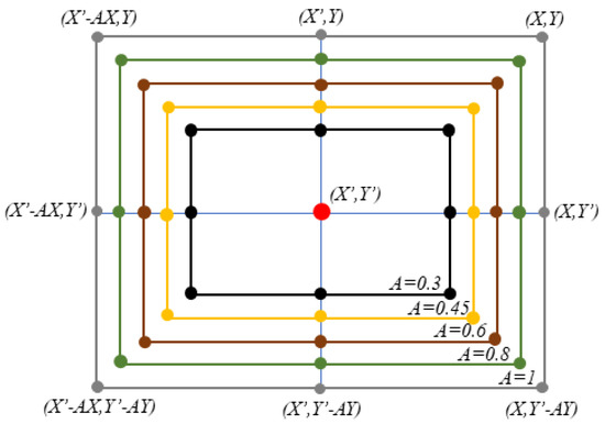
Figure 1.
The model of the decreasing enclosing mechanism.
The decreasing enclosing mechanism can simulate whale populations enclosing and randomly pursuing prey. To achieve this mathematical model, the shrinking enclosing mechanism alters the search mode through the coefficient vector A. Figure 1 depicts a model of the decreasing enclosing mechanism. Among these, represents the current position of the search agent, and (X,Y) represents the current ideal value. Figure 1’s coefficient vector A can guide search agents through the exploitation or exploration phase. When , the search agent can approach the current optimum value, demonstrating the algorithm’s capacity for local exploitation. The decreasing enclosing method allows the algorithm to successfully balance exploitation and exploration by closing or spreading the best value area.
2.2. The Spiral Update Mechanism
The mechanism of shrinking and wrapping means the surrounding circle of food will gradually shrink during the predation process of whales. The whales swim in a spiral around the food when they shrink and surround the food, which is the spiral position update. The spiral position update can be expressed as
where b is a constant that can alter the shape of the spiral and l is a uniformly distributed random value in the interval . The process of the entire spiral update can be represented by the model in Figure 2:
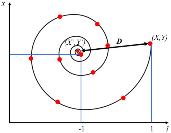
Figure 2.
The model of the spiral updating mechanism.
When whales shrink and surround the food, the spiral position updates meanwhile. It is necessary to assume that each behavior has a certain probability when using a mathematical model to describe this behavior. The specific mathematical motion model of this behavior is as follows
where p is a random number uniformly distributed in [0, 1].
2.3. Random Search Location Update
To improve whales’ global search abilities, a certain degree of randomness is required when seeking for prey, which can broaden the search area of whale groups. When the coefficient , the whales are outside the shrinking encirclement, and the random search method should be used. When the coefficient , the whales are inside the shrinking encirclement, and the spiral encircling search method should be used. The random search update formula is:
where is a random location of the whale. The combination of the above three search methods constitutes the whale optimization algorithm.
2.4. Flow of Whale Optimization Algorithm
The pseudo code of the whale algorithm is shown in Algorithm 1:
| Algorithm 1 whale algorithm |
|
3. Improved Whale Optimization Algorithm
Based on the standard WOA, the proposed IWOA improves the strategy optimization in three aspects: adaptive weight, spiral coefficient optimization, and optimal neighborhood perturbation.
3.1. Adaptive Weight
The concept of inertia weight first appeared in the particle swarm algorithm, which means the change of particle coordinates is related to inertia weight in the iteration of particle swarm optimization [27].
This inspires the addition of an inertia weight w that modifies the position update of IWOA according to the quantity of iterations. The influence of the optimal whale position on the present individual position adjustment needs to be reduced in the early stages of the algorithm search in order to increase global search capability. The influence of the ideal whale position will steadily improve as the number of iterations increases, encouraging other whales to fast converge to the ideal whale position, allowing for an acceleration of convergence speed. The adaptive inertia weight made up of iteration number t is chosen as follows depending on the change in the whale optimization algorithm’s update count:
The position update formula of IWOA is:
After the adaptive weight is implemented, the position update will dynamically alter the weight based on the rise in the number of iterations, allowing the best whale position to steer different whales at different times. The whale group will concentrate on the direction of the optimal position with the increase in the number of iterations, and the larger weight will make the whale position move faster, thereby speeding up the algorithm convergence speed.
3.2. Helix Factor Optimization
When the whale’s spiral position is updated, the coefficient b controls the radian of the spiral update. The coefficient b is a fixed constant in the standard whale algorithm, which makes the whale move according to a fixed spiral radian when searching for prey in a spiral. A single method of movement makes it simple to converge on a local optimal solution, hence diminishing the algorithm’s capacity for global search.
As a result, parameter b is also designed as a variable that changes with the number of iterations, allowing the spiral curve of the whale to be dynamically adjusted during the spiral search, increasing the whales’ ability to explore unknown areas and thus improving the algorithm’s global search ability. The new adaptive weight spiral position update formula is as follows:
The helix mathematical model is used to design the parameter b. The shape of the helix is dynamically modified based on the initial helix model by introducing the number of iterations. During iterations, the spiral’s shape changes from large to small when the specified parameter b is increased.
In the early stages of the algorithm, the whales hunt for targets in a greater spiral form to explore the global ideal solution as much as possible in order to improve the algorithm’s global optimal search ability. The whales hunt for targets in a narrow spiral shape later in the algorithm to improve the precision of the optimization method.
3.3. Optimal Neighborhood Perturbation
The whales will take the optimal position of the current position as the iteration target each time when updating its position. In each iteration process, the whale’s position will only be updated when a better solution appears, which will result in higher probability of not updating position in the later iterations of evolution, and then the search efficiency of the entire algorithm will reduce.
As a result, IWOA employs the optimal neighborhood perturbation technique and searches again near the optimal position to obtain a better global value, which not only improves the algorithm’s convergence speed but also prevents the algorithm from prematurely aging. A random disturbance is generated in the best possible location to boost its search for nearby space. The neighborhood disturbance formula is as follows:
where limits the range of Gaussian random numbers between [, 1]; is a uniformly generated random number between [0, 1], is the generated new location.
A greedy strategy is adopted to determine whether to retain the generated neighborhood positions, and the corresponding formula is as follows:
where is the adaptive value of the x position. The original position will be replaced if the generated position is better, otherwise, the optimal position remains the global optimum.
3.4. IOWA Algorithm Flow
The algorithm flow chart of the IOWA algorithm is shown in Figure 3:
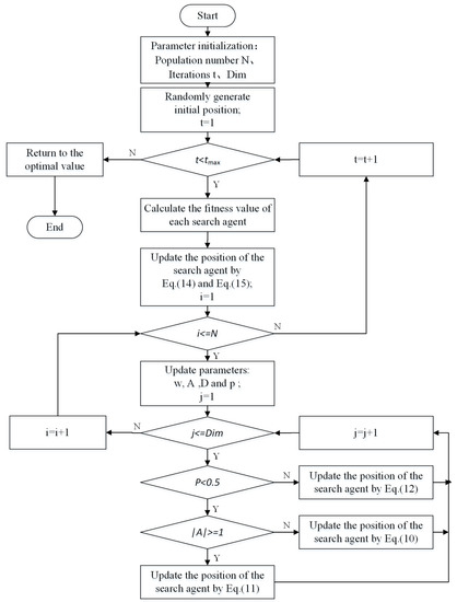
Figure 3.
The flowchart of IWOA.
The pseudo code of IWOA is shown in Algorithm 2.
| Algorithm 2 IWOA |
|
3.5. Algorithm Complexity Analysis
The time complexity of an algorithm is a function that qualitatively reflects the method’s running time. The number and structure of the arithmetic unit influence the time complexity of an optimization algorithm.
The number of search agents, iterations, and the location update method largely affect the temporal complexity of WOA. The following is the analysis and comparison of the time complexity of WOA and IWOA:
- In the standard whale optimization algorithm, the time complexity of the WOA can be obtained as by setting the size of whales in the algorithm as N, the problem dimension as D, and the maximum number of iterations as T.
- The IWOA introduces three improved strategies on the basis of the original algorithm, but the number of cycles of the algorithm does not increase after adding the adaptive weight and variable spiral update strategy, which can be known from the above algorithm modification process. Thus, the time complexity of the IWOA can be obtained as . Adding the optimal neighborhood perturbation adds a cycle of traversing the population to the periphery of the algorithm, thus, the amount of computation increases by .
- The increased operation amount will not cause too much computational burden to the time complexity of the entire algorithm, therefore the overall time complexity of the IWOA is the same as that of the standard WOA.
Space complexity is used to judge the memory space requirement of an algorithm. The space complexity here is mainly determined by the size of the whale and the dimension of the problem to be solved. Therefore, the IWOA does not increase the space complexity.
4. Performance Analysis
Since numerous factors are required to be optimized, the reliability analysis ought to be performed prior to array antenna pattern synthesis. According to Wolpert’s “No Free Lunch” (NFL) theorem [28], there is no algorithm that can solve all issues of all sectors worldwide. To confirm the efficacy of the IWOA method, four well-known test functions are selected, which are also utilized as benchmark functions for GA and PSO optimization techniques. The benchmark functions are listed in Table 1. To validate the IWOA algorithm’s efficiency, four well-known test functions are chosen, which are also used as benchmark functions for optimization strategies such as GA and PSO. Table 1 displays the benchmark functions.

Table 1.
This is a wide table.
The GA, PSO, DE, IWO, MOA, standard WOA algorithms, and IWOA algorithms were simulated and compared in 30 dimensions using the aforementioned four standard test functions. The computed can be defined as the fitness value of the solution. In the procedure described, the population size is set to 40 and the maximum number of iterations is 500. Table 2 illustrates the parameters of several algorithms. Additionally, tests were performed 30 times separately to prevent random deviation.The population size in the above algorithm is set to the same 40, and the maximum number of iterations is 500. The parameters of different algorithms are shown in Table 2. Furthermore, tests are independently repeated 30 times to avoid random deviation.
Table 2.
Parameter setups of different algorithms.
Table 3 presents the results of thirty different tests computed by various methods. Ideal value, average value, and variance are the three statistical indicators, which are used to evaluate the optimization accuracy, average accuracy, and robustness of the algorithm in turn. The best results are indicated in bold for each function. The aforementioned three indicators of IWOA algorithm are obviously superior to other algorithms. Therefore, compared with other algorithms, IWOA has the optimal overall performance in solving the solution problem of the above four test functions, as shown in Table 3. As a result, compared with other algorithms, IWOA has the most satisfying overall performance in solving these four test functions listed above.
Table 3.
Results of algorithms on basic benchmark functions.
Correspondingly, Figure 4a–d show the convergence curves of different algorithms in the process of solving the above test functions. It can be seen that the IWOA has a faster convergence and better solution result.
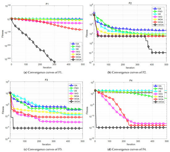
Figure 4.
Simulation experiment results.
However, the performance of the IWOA algorithm in sidelobe suppression optimization problem needs further evaluation.
5. Application of IWOA in the Array Antenna Pattern Synthesis
5.1. Signal Model of the Planar Phased Array Antenna
Consider the planar phased array composed of N array elements shown in Figure 5, its far-field radiation pattern is
where is the element pattern function, , is the wavelength, is the coordinate position of the nth array element, and is the amplitude excitation factor and phase excitation factor of the corresponding array element.
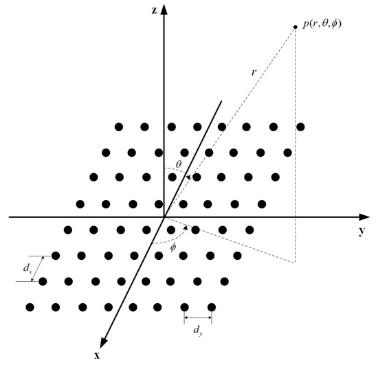
Figure 5.
The planar phased array model.
In this paper, the IOWA is applied to the actual engineering project. Since the RF device of the antenna can only control the amplitude within a maximum range of 20 dB, we need to restrict the amplitude variation within 20 dB in the process of the pattern synthesis. In engineering applications, Wilkinson circuit is usually used to realize the signal combination. The combining circuit of small signal is narrow and can achieve a high machining accuracy, which makes sure the amplitude change can be controlled more accurately. In addition, since the power of each signal is not equal, the combination efficiency will be affected when the power difference is large, and the hardware will also be more difficult to design. Therefore, we must control the range of amplitude change within 20 dB. Of course, if the amplitude change is too small, the sidelobe suppression will be very poor. In practice, we achieve the attenuation control by using attenuators.
The optimization goal is to achieve sidelobe suppression only by optimizing the amplitude of the excitation. The designed fitness function can be expressed as
where is the calculated gain of the main lobe pointing angle, is the designed gain of the main lobe pointing angle, is the calculated maximum sidelobe level among the entire pattern range, is the designed maximum sidelobe level, and are two weight coefficients, and in the design.
5.2. Result Analysis
The array element adopts the traditional single-layer microstrip antenna and uses the coaxial feeding mode. The radiation patch is nearly square with a half wavelength in length. As shown in Figure 6, the patch is symmetrically chamfered in the center to ensure that the antenna radiates circularly polarized waves. Simulation results show that the gain of the antenna at the center frequency is 7.5 dBi and the axial ratio is 0.3 dB. It has favorable circularly polarized radiation characteristics and meets the performance requirements of array element antenna. The radiation pattern of the array element is shown in Figure 7.
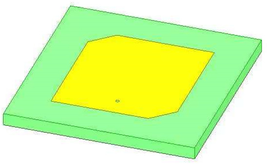
Figure 6.
Microstrip antenna model.

Figure 7.
Radiation pattern of array element.
For the 64-element planar array antenna shown in Figure 8, the frequency is set to 30 GHz, and the unit patterns of all elements are imported through the simulation software HFSS. We control the range of amplitude variation within 20 dB. In the actual engineering project, we design a two-stage amplitude-phase control chip. A 6-bit digital attenuator is used to achieve a 20 dB amplitude control, and the beamformer sends instructions through the wave control interface. The chip is integrated with 6-bit phase shifter, 6-bit attenuator, gain module, power divider, serial-parallel converter, and power modulation circuits. The block diagram of the chip is shown in Figure 9.
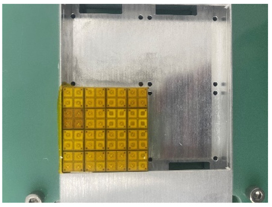
Figure 8.
A 64-element planar phased array antenna.
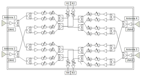
Figure 9.
Block diagram of the amplitude-phase control chip.
Subsequently, the GA, PSO, DE, IWO, MOA, standard WOA, and IWOA are carried out for sidelobe suppression optimization. The parameter design of each algorithm is shown in Table 2. Each algorithm iterated 2000 times and repeated 20 times independently to ensure the reliability of the experiment.
To compare the performance of these algorithms more intuitively, the average convergence results of 20 independent experiments are provided in Figure 10. It can be seen that the convergence speed of IWOA is significantly faster than other algorithms, and the final solution is also better than the others.
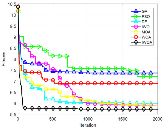
Figure 10.
Convergence rates of the 64-element planar phased array.
Owing to the requirement of engineering implementation, the range of amplitude excitation is limited in the algorithm. The amplitude attenuation is controlled between 0 to 20 dB. Since the minimum amplitude attenuation step in our chip can only reach 0.5 dB, we carried out a quantization process before obtaining the result of each iteration of the algorithm. Then, the result obtained after quantization is used as the required solution and the optimal solution is obtained after continuous iterations. In terms of engineering implementation, we take the optimal solution of the proposed algorithm as input and use a 6-bit digital attenuator to achieve the amplitude control. Corresponding instructions are sent by the beamformer through the wave control interface. The arrangement of the 64-element planar array antenna is shown in the following Figure 11, and the optimal solution obtained through the proposed algorithm is shown in Table 4.
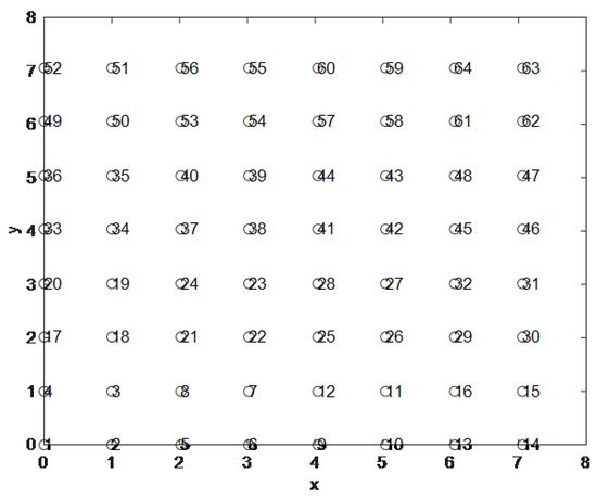
Figure 11.
Positions of the 64-element planar phased array antenna.
Table 4.
The associated amplitude excitation attenuation of 64-element planar phased array antenna.
The optimal solution of the above seven algorithms for sidelobe level suppression problem is determined, and the corresponding 2D antenna pattern diagrams are shown in Figure 12, where the maximum sidelobe of the conventional pattern is −11.05 dB without adjusting the amplitude, while the maximum sidelobe obtained by IWOA optimization is −22.87 dB, illustrating the great performance of IWOA for sidelobe suppression. Figure 13 portrays the 3D antenna pattern diagram synthesized by IWOA.
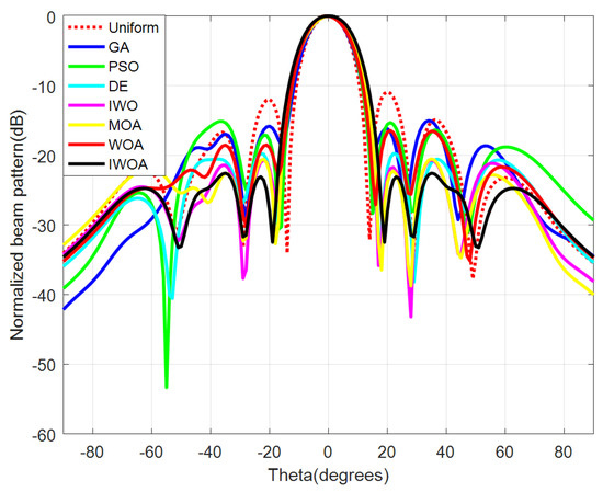
Figure 12.
The 2D beam patterns of the 64-element planar phased array.
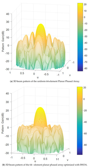
Figure 13.
3D beam patterns of 64−element planar phased array.
The optimal value, average value, and variance of 20 independent experiments are shown in Table 5. After IWOA optimization, the optimal MSLL reaches −23.09 dB, the worst MSLL is −22.53 dB, and the standard deviation of 20 experiments is 0.25. It can be seen that the IWOA algorithm performs better in optimization results and robustness through the comparison with other algorithms in Table 5.
Table 5.
Simulation results obtained by IWOA and other optimization algorithms.
In the simulation model mentioned above, the coupling among the array elements is not considered. Therefore, EM simulations must be performed to determine whether the proposed technique can successfully optimize the maximal sidelobe in the presence of coupling.
The electromagnetic simulations are performed using ANSYS electromagnetics. The amplitude excitation obtained through algorithm optimization in MATLAB is input into the 64-element planar array antenna model designed by HFSS software to verify the feasibility of the optimization algorithm in practical engineering.
Figure 14a shows the comparison of 2D beam optimization effects of each algorithm obtained through EM simulation, depicting the 2D EM simulation results in 0 planes. The first sidelobe optimized by the IWAO is −18.03 dB, and the second sidelobe level is −22.2 dB. Figure 14b is the 2D EM simulation results in 90 planes. The first sidelobe optimized by the IWAO is −18.71 dB, and the second sidelobe level is −19.5 dB. Obviously, IWOA has the best sidelobe suppression performance compared with other algorithms. The sidelobe suppression performance of HFSS simulation results has deteriorated to a certain extent after the addition of coupling, yet both simulations still prove the effectiveness of the IWOA.
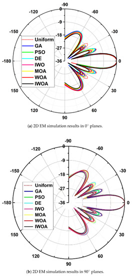
Figure 14.
The 2D EM simulation results.
Since the primary consideration in engineering is to solve the problem of interference avoidance, sidelobe suppression is the first optimization goal. Meanwhile, the beam width will also be broadened to some extent when performing sidelobe suppression. Through simulation analysis, the beam broadening after sidelobe suppression is within the acceptable range of the engineering as well. Table 6 shows the maximum SLL and beamwidth of the compared algorithms.
Table 6.
The maximum SLL and beamwidth of the compared algorithms.
Figure 15a and Figure 15b, respectively, show the 3D waveform diagrams of 64 array elements before and after optimization. The color of the maximum sidelobe becomes lighter, indicating that the value is significantly smaller, which proves that the maximum SLLs have been significantly optimized.
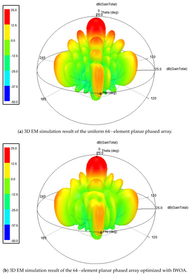
Figure 15.
The 3D EM simulation results.
6. Conclusions
Aiming at the design requirements of low sidelobe level of spaceborne phased array antenna, an improved IWOA algorithm based on a standard WOA algorithm is proposed. It has three improvement strategies, which are adaptive weight, spiral coefficient optimization, and optimal neighborhood perturbation. The superiority of IWOA is proved by comparing with other algorithms in the simulation experiment with classical test functions as the validation criteria. In addition, the IWOA is effectively used for antenna synthesis of a 64-element planar array antenna. IWOA outperforms GA, PSO, DE, IWO, MOA, and regular WOA in terms of convergence speed and optimization outcomes when applied to the sidelobe level suppression issue. Ultimately, the practicability and effectiveness of IWOA are verified through the electromagnetic field simulation with coupling added.
Author Contributions
Authors contributed as follows: Conceptualization, H.H., H.L. and L.Z.; Methodology, H.H., H.L. and X.J.; Investigation, H.H. and J.Y.; Supervision, Y.Z., J.Y. and L.Z.; writing—original draft preparation, H.H. and X.J.; writing—review and editing, L.Z.; project administration, H.H. All authors have read and agreed to the published version of the manuscript.
Funding
This work was supported in part by the National Natural Science Foundation of China (grant number U21A20443). Shanghai Industrial Collaborative Innovation Project (grant number XTCX-KJ-2022-02).
Institutional Review Board Statement
Not applicable.
Informed Consent Statement
Not applicable.
Data Availability Statement
Not applicable.
Conflicts of Interest
The authors declare no conflict of interest.
References
- Ha, B.V.; Mussetta, M.; Pirinoli, P.; Zich, R.E. Modified Compact Genetic Algorithm for Thinned Array Synthesis. IEEE Antennas Wirel. Propag. Lett. 2016, 15, 1105–1108. [Google Scholar] [CrossRef]
- Angeletti, P.; Berretti, L.; Maddio, S.; Pelosi, G.; Selleri, S.; Toso, G. Phase-Only Synthesis for Large Planar Arrays via Zernike Polynomials and Invasive Weed Optimization. IEEE Trans. Antennas Propag. 2022, 70, 1954–1964. [Google Scholar] [CrossRef]
- Panigrahi, S.; Chou, H.-T.; Chang, C.-Y. Radiation pattern nulling in phased array antennas using superior discrete fourier transform and Dolph-Tschebyscheff based synthesis techniques. Radio Sci. 2022, 57, 1–14. [Google Scholar] [CrossRef]
- Prado, D.R. The Generalized Intersection Approach for Electromagnetic Array Antenna Beam-Shaping Synthesis: A Review. IEEE Access 2022, 10, 87053–87068. [Google Scholar] [CrossRef]
- Lin, Z.; Hu, H.; Lei, S.; Li, R.; Tian, J.; Chen, B. Low-Sidelobe Shaped-Beam Pattern Synthesis With Amplitude Constraints. IEEE Trans. Antennas Propag. 2022, 70, 2717–2731. [Google Scholar] [CrossRef]
- Yang, F. Synthesis of Low-Sidelobe 4-D Heterogeneous Antenna Arrays Including Mutual Coupling Using Iterative Convex Optimization. IEEE Trans. Antennas Propag. 2020, 68, 329–340. [Google Scholar] [CrossRef]
- Lin, Z.; Hu, H.; Chen, B.; Lei, S.; Tian, J.; Gao, Y. Shaped-Beam Pattern Synthesis With Sidelobe Level Minimization via Nonuniformly-Spaced Sub-Array. IEEE Trans. Antennas Propag. 2022, 70, 3421–3436. [Google Scholar] [CrossRef]
- Wang, A.; Li, X.; Xu, Y. BA-Based Low-PSLL Beampattern Synthesis in the Presence of Array Errors. IEEE Access 2022, 10, 9371–9379. [Google Scholar] [CrossRef]
- Liang, Z.; Ouyang, J.; Yang, F. A hybrid GA-PSO optimization algorithm for conformal antenna array pattern synthesis. J. Electromagn. Waves Appl. 2018, 32, 1601–1615. [Google Scholar] [CrossRef]
- Anjaneyulu, G.; Siddartha Varma, J. Synthesis of Low Sidelobe Radiation Patterns from Embedded Dipole Arrays Using Genetic Algorithm. Sustain. Commun. Netw. Appl. 2020, 39, 791–797. [Google Scholar]
- He, M.; Zheng, Z.; Wang, W.Q.; Kang, Z. Pattern synthesis for uniform linear array using genetic algorithm and artificial neural network. Multidimens. Syst. Signal Process. 2022, 33, 263–273. [Google Scholar] [CrossRef]
- Li, H.; Jiang, Y.; Ding, Y.; Tan, J.; Zhou, J. Low-Sidelobe Pattern Synthesis for Sparse Conformal Arrays Based on PSO-SOCP Optimization. IEEE Access 2018, 6, 77429–77439. [Google Scholar] [CrossRef]
- Hiroshi, H.; Naobumi, M.; Hisashi, M.; Hiroyuki, A. Array antenna pattern synthesis for fixed amplitude and limited phase range using genetic algorithm. IEICE Commun. Express 2021, 10, 721–725. [Google Scholar]
- Kang, M.S.; Won, Y.J.; Lim, B.G.; Kim, K.T. Efficient Synthesis of Antenna Pattern Using Improved PSO for Spaceborne SAR Performance and Imaging in Presence of Element Failure. IEEE Sens. J. 2018, 18, 6576–6587. [Google Scholar] [CrossRef]
- Cui, C.Y.; Jiao, Y.C.; Zhang, L. Synthesis of Some Low Sidelobe Linear Arrays Using Hybrid Differential Evolution Algorithm Integrated With Convex Programming. IEEE Antennas Wirel. Propag. Lett. 2017, 16, 2444–2448. [Google Scholar] [CrossRef]
- Das, A.; Mandal, D.; Ghoshal, S.P.; Kar, R. Moth flame optimization based design of linear and circular antenna array for side lobe reduction. Int. J. Numer. Model. Electron. Netw. Devices Fields 2018, 32, 1–15. [Google Scholar] [CrossRef]
- Darvish, A.; Ebrahimzadeh, A. Improved Fruit-Fly Optimization Algorithm and Its Applications in Antenna Arrays Synthesis. IEEE Trans. Antennas Propag. 2018, 66, 1756–1766. [Google Scholar] [CrossRef]
- Zheng, T. IWORMLF: Improved Invasive Weed Optimization With Random Mutation and Lévy Flight for Beam Pattern Optimizations of Linear and Circular Antenna Arrays. IEEE Access 2020, 8, 19460–19478. [Google Scholar] [CrossRef]
- Li, X.; Luk, M.K. The Grey Wolf Optimizer and Its Applications in Electromagnetics, in IEEE Transactions on Antennas and Propagation. J. Korean Inst. Commun. Inf. Sci.. 2020, 68, 2186–2197. [Google Scholar]
- Owoola, E.O.; Xia, K.; Wang, T.; Umar, A.; Akindele, R.G. Pattern Synthesis of Uniform and Sparse Linear Antenna Array Using Mayfly Algorithm. IEEE Access 2021, 9, 77954–77975. [Google Scholar] [CrossRef]
- Pinchera, D.; Migliore, M.D.; Schettino, F.; Lucido, M.; Panariello, G. An Effective Compressed-Sensing Inspired Deterministic Algorithm for Sparse Array Synthesis. IEEE Trans. Antennas Propag. 2018, 66, 149–159. [Google Scholar] [CrossRef]
- Singh, U.; Kumar, H.; Kamal, T.S. Design of Yagi-Uda Antenna Using Biogeography Based Optimization. IEEE Trans. Antennas Propag. 2010, 58, 3375–3379. [Google Scholar] [CrossRef]
- Baumgartner, P. Multi-Objective Optimization of Yagi–Uda Antenna Applying Enhanced Firefly Algorithm With Adaptive Cost Function. IEEE Trans. Magn. 2018, 54, 1–4. [Google Scholar] [CrossRef]
- Quevedo-Teruel, O.; Rajo-Iglesias, E. Ant Colony Optimization in Thinned Array Synthesis With Minimum Sidelobe Level. IEEE Antennas Wirel. Propag. Lett. 2006, 5, 349–352. [Google Scholar] [CrossRef]
- Mirjalili, S.; Lewis, A. The whale optimization algorithm. Adv. Eng. Softw. 2016, 95, 51–67. [Google Scholar] [CrossRef]
- Zhang, C.; Fu, X.; Ligthart, L.P.; Peng, S.; Xie, M. Synthesis of Broadside Linear Aperiodic Arrays With Sidelobe Suppression and Null Steering Using Whale Optimization Algorithm. IEEE Antennas Wirel. Propag. Lett. 2018, 17, 347–350. [Google Scholar] [CrossRef]
- Chrouta, J.; Farhani, F.; Zaafouri, A. A modified multi swarm particle swarm optimization algorithm using an adaptive factor selection strategy. Trans. Inst. Meas. Control. 2021, 01423312211029509. [Google Scholar] [CrossRef]
- Ho, Y.; Pepyne, D. Simple Explanation of the No-Free-Lunch Theorem and Its Implications. J. Optim. Theory Appl. 2002, 115, 549–570. [Google Scholar] [CrossRef]
- Greda, L.A.; Winterstein, A.; Lemes, D.L.; Heckler, V.T. Beamsteering and Beamshaping Using a Linear Antenna Array Based on Particle Swarm Optimization. IEEE Access 2019, 7, 141562–141573. [Google Scholar] [CrossRef]
- Sun, G.; Liu, Y.; Li, H.; Liang, S.; Wang, A.; Li, B. An antenna array sidelobe level reduction approach through invasive weed optimization. Int. J. Antennas Propag. 2018, 2018, 4867851–4867867. [Google Scholar] [CrossRef]
Disclaimer/Publisher’s Note: The statements, opinions and data contained in all publications are solely those of the individual author(s) and contributor(s) and not of MDPI and/or the editor(s). MDPI and/or the editor(s) disclaim responsibility for any injury to people or property resulting from any ideas, methods, instructions or products referred to in the content. |
© 2023 by the authors. Licensee MDPI, Basel, Switzerland. This article is an open access article distributed under the terms and conditions of the Creative Commons Attribution (CC BY) license (https://creativecommons.org/licenses/by/4.0/).