Article

Hybrid EWMA Control Chart under Bayesian Approach Using Ranked Set Sampling Schemes with Applications to Hard-Bake Process

1
Department of Statistics, Abdul Wali Khan University Mardan, Mardan 23200, Pakistan
2
Department of Statistics, Comsats University Islamabad, Lahore 57000, Pakistan
3
Department of Mathematical Sciences, College of Science, Princess Nourah bint Abdulrahman University, P.O. Box 84428, Riyadh 11671, Saudi Arabia
4
Department of Statistics, Quaid-i-Azam University, Islamabad 44000, Pakistan
*
Author to whom correspondence should be addressed.
Appl. Sci. 2023, 13(5), 2837; https://doi.org/10.3390/app13052837
Submission received: 26 January 2023 / Revised: 13 February 2023 / Accepted: 17 February 2023 / Published: 22 February 2023

Abstract

:
A memory-type control chart is an important tool of statistical process control for monitoring small to moderate shifts in the manufacturing process. Using the prior information by the Bayesian approach is helpful in control charts. In this paper, a new hybrid exponentially weighted moving average (HEWMA) control chart is suggested under the Bayesian theory using ranked set sampling (RSS) schemes for posterior and posterior predictive distribution with informative prior and different loss functions (LFs). The extensive Monto Carlo simulation is conducted to evaluate the overall performance of the proposed Bayesian HEWMA control chart through average-run-length (ARL) and standard-deviation of the run-length (SDRL). Finally, a numerical example of the hard-bake process in semiconductor manufacturing is used to check the working and execution of the proposed Bayesian HEWMA control-chart under different RSS schemes. The results reveal that the suggested Bayesian HEWMA control-chart under RSS schemes is more sensitive in detecting out-of-control signals than the Bayesian HEWMA and Bayesian AEWMA control-charts under simple random sampling.

1. Introduction

Statistical process control (SPC) offers a variety of tools for monitoring process parameters to maintain and improve the quality of the products by reducing variations in the manufacturing process. There could be two types of variabilities, one is called a common or natural source of variability, and the second is called an assignable source variability. Natural sources of variability are impossible to control without revising the whole process, so the work under those conditions is considered to be in-control. If the production process has an assignable source of variation, it is out-of-control. In manufacturing industries, variations are integral components of the running processes. The statistical quality control charts are the most important and powerful SPC technique that is commonly used in many service industries to monitor manufacturing processes. The main objective of the statistical quality control chart is to maintain the process stability by detecting the infrequent variations in the production process, making it possible for the control system to take the necessary corrections before the manufacturing of the non-conforming items. The fundamental features of SPC are also the identification and monitoring of special causes of variation in the production process, which improves the quality of the final product. In the 1920s the concept of the quality control chart was first introduced by Walter A. Shewhart [1]. This idea served as the foundation for the contemporary SPC, with some modifications made afterward. The cumulative sum (CUSUM) suggested by Page [2] and the exponentially weighted moving average (EWMA) suggested by Roberts [3] control charts are the most popular and sophisticated statistical process monitoring tools of SPC. The CUSUM and EWMA charts are both memory-type control charts, whereas the classical Shewhart control chart is a memoryless type control chart. Both memory-type and memoryless control charts provide excellent detection of small/moderate and large changes in the process parameter(s). Often, process and service industries use memory-type control charts to detect small to moderate process disturbances, which can have serious financial consequences. The Shewhart control chart is more effective than the CUSUM and EWMA control chart when it comes to detecting large changes in the process parameters. Many authors have worked on the memory-type control chart, such as Lucas and Crosier [4], Khoo [5], Khan et al. [6], and Saghir et al. [7]. Adeoti et al. [8] studied the hybrid homogeneously weighted moving average (HWMA) control chart for the process mean by combining two HWMA control charts. The results show that the hybrid HWMA control chart is more sensitive than the existing control charts. Arslan et al. [9] suggested an improved adaptive EWMA control chart for monitoring the process location, the unknown shift is estimated by the HEWMA statistic. They used the ARL, extra quadratic loss, and relative ARL for performance evaluation and the comparison revealed the superiority of the proposed control chart. A Bayesian multivariate control chart with different LFs was suggested by Tsui and Woodall [10]. Menzefricke [11] and Menzefricke [12] suggested the Bayesian control chart for the process mean and dispersion, respectively. Tian and Wu [13] proposed a CUSUM control chart for mean and variance to detect the variation in the production process. Serel [14] studied the EWMA control chart for the mean and dispersion of a process with different LFs, such as quadratic, linear, and exponential LFs. EWMA control chart under Bayesian approach for posterior and posterior predictive distribution using different LFs and with informative and non-informative prior distribution suggested by Riaz et al. [15]. Noor et al. [16] proposed a Bayesian HEAWA control chart for monitoring the process mean using an informative prior distribution with different LFs. The performance of the suggested control chart was evaluated through the ARL and SDRL. Tang et al. [17] suggested a new risk priority model using the belief Jensen–Shannon divergence and entropy measure in the evidence theory. The effectiveness and partibility of the suggested method were verified by using a case study on the sheet steel production process. Lin et al. [18] proposed the Bayesian EWMA control chart to efficiently detect the process variance of a distribution-free process. They explored the good sampling properties of the suggested statistic, which is suitable for monitoring the time-varying process distribution, and showed the efficiency of the control chart through a simulation study. The adaptive EWMA (AEWMA) control chart using the Bayesian approach was suggested by Noor et al. [19], who also studied the effect of LFs on the considered control charts by using ARLs and SDRLs.
All these works were created for classical and Bayesian approaches based on SRS. Our motivation in this article is to propose a Bayesian HEWMA control chart using different RSS schemes under two LFs, i.e., squared error LF (SELF) and linex LF (LLF) for posterior and posterior predictive distribution. A Monto Carlo simulation study is performed to evaluate the working and execution of the proposed Bayesian HEWMA control chart under RSS schemes. Section 2 consists of an introduction to the Bayesian approach and LFs. The different RSS schemes are discussed in Section 3. The construction of the proposed Bayesian HEWMA control chart under different RSS schemes is discussed in Section 4. A simulation study is included in Section 5, Section 6 gives a results discussion and the main findings of the proposed Bayesian HEWMA control chart with Bayesian HEWMA and the Bayesian AEWMA control chart under simple random sampling. Section 7 contains the real data application of the proposed control chart. Section 8 of the article contains the conclusion.

2. Bayesian Approach

The Bayesian approach is the method of estimation for unknown population parameters which utilizes both sample and prior information. The prior distribution is our beliefs about the unknown population parameter before some information is taken into account. The prior information is broadly divided into two-parts (i) informative prior and (ii) non-informative prior. The prior distribution of the parameter that has some known information regarding an unknown population parameter is called the informative prior, if the prior and sampling distribution belongs to the same family of distribution it is called the conjugate prior. In this study, the study variable X with mean θ and variance δ 2 with the in-control process and taking the conjugate prior (normal prior) with parameters θ 0 and δ 0 2 is defined as follows:
p ( θ ) = 1 2 π δ 0 2 exp { 1 2 δ 0 2 ( θ θ 0 ) 2 }
while if nothing is known about the population parameter, it is said to be a non-informative prior, which has less effect on the posterior distribution, and in this case, the prior distribution is proportional to the uniform distribution. The probability function p ( θ ) represents the uniform prior distribution given by
p ( θ ) n δ 2 = c n δ 2
where c is the proportionality constant.
In the case of the uniform prior, the invariance property does not exist, thus Jeffrey [20] proposed the prior function which is proportional to the Fisher information matrix. The prior probability function suggested by Jeffrey is given below:
p ( θ ) I ( θ )
where I ( θ ) denotes the Fisher information matrix.
The posterior distribution which is based on the combination of a sample and a prior distribution for a population parameter θ is defined as follows:
p ( θ / x ) = p ( x θ ) p ( θ ) p ( x θ ) p ( θ ) d θ
For a new data set Y, the posterior predictive distribution based on posterior distribution is given by
p ( y / x ) = p ( y θ ) p ( θ / x ) d θ
The LFs play a vital role in the Bayesian inference which is used to reduce the risk related to the Bayes estimator. The two different LFs such as symmetric (SELF) and asymmetric (LLF) have been used in this study.

2.1. Squared Error Loss Function

The SELF is a symmetric type of LF proposed by Gauss [21]. Consider the study variable X and estimator θ ^ which is used to estimate the unknown population parameter θ , then the SELF is defined as
L ( θ , θ ^ ) = ( θ θ ^ ) 2
and the Bayes estimator based on SELF is given by
θ ^ = E θ / x ( θ )

2.2. Linex Loss Function

Varian [22] proposed the LLF as an asymmetric LF, which is used for the estimation of location parameters more efficiently because it minimizes the risk associated with the Bayes estimator. The LLF is given by
L ( θ , θ ^ ) = ( e c ( θ θ ^ ) c ( θ θ ^ ) 1 )
where θ ^ is a Bayes estimator for an unknown population parameter θ , defined as
θ ^ = 1 c I n E θ / x ( e c θ )

3. Ranked Set Sampling

McIntyre [23] proposed a sampling design named a ranked set sampling scheme (RSS), which is used to estimate population parameters more efficiently. In the RSS method, the m2 units from the considered population are selected and distributed to m sets with similar sizes m. The units of the study variable can be ordered (ranked) based on eye inspection or with the help of an auxiliary variable without considering the actual measurement. After ranking units in all sets, the first unit is picked from the first set and the second is picked from the second set and measured, the process continues until the largest unit is selected from the last set. This completes one cycle of RSS; if needed, the whole procedure is repeated r times to complete the required sample n = r m . The procedure of the RSS is demonstrated as Z i ( j ) , r , i , j = 1, 2, 3 … m; r = 1, 2, 3 … c, be the jth order statistic in the ith sample set with cycle r. The mean and variance of the ranked set sample estimator for c = 1 are as follows:
Z ¯ ( R S S ) = 1 m i = 1 m Z i ( i )
with variance
var ( Z ¯ ( R S S ) ) = δ 2 m 1 m 2 i = 1 m ( μ ( i ) μ )

3.1. Median Ranked Set Sampling

Muttalk [24] suggested a modified version of the RSS scheme called Median RSS (MRSS), which efficiently estimates the population mean by minimizing error in ordering. The complete procedure of MRSS is as follows:
Similar to RSS, we acquired m 2 units from the underlying population randomly and distributed them to m sets of the same size m and all the m units within each set are ordered with the help of the variable under study.
In the second step, if m is odd, then draw middle units, i.e., ( ( m + 1 ) 2 ) t h from all the sets selected as samples. In case when m is even, select the lowest ordered units from the two middle sampling units of the first ( m 2 ) t h sets and draw the largest ordered units from the two middle sampling units remaining ( m 2 ) t h .
1.
The above two steps complete one cycle of MRSS of size m ; if needed, repeat the whole method r times to meet the requirement.
The estimator for the population mean of MRSS of one cycle when the sample size is odd is defined as follows:
Z ¯ ( M R S S ) O = 1 m ( i = 1 m Z i ( m + 1 2 ) )
with variance
var ( Z ¯ ( M R S S ) O ) = 1 m ( δ ( m + 1 2 ) 2 ) .
In a situation when the sample size is even, the estimator of a population mean of MRSS with one cycle is
Z ¯ ( M R S S ) O = 1 m ( i = 1 m 2 Z i ( m 2 ) + i = 1 m 2 Z m 2 + i ( m + 1 2 ) )
with variance
var ( Z ¯ ( M R S S ) O ) = 1 m ( δ ( m 2 ) 2 + δ ( m + 2 2 ) 2 ) .

3.2. Extreme Ranked Set Sampling

Another modified RSS scheme, Extreme RSS (ERSS), was suggested by Samawi et al. [25]. The ERSS scheme is useful when selecting an ordered unit is a hard task rather than an extreme unit. The complete method for selecting ERSS is as follows:
1.
We drew m 2 units randomly from the available population and allocated all these units into m sets with the same set size m , units in each set are ranked with the help of the study variable.
2.
If m is even, then select the lowest units for measurement from the first ( m 2 ) ordered sets and the largest units from the last ranked sets, if m is odd then draw the lowest units from the first ( m 1 2 ) ordered sets and the largest units from the remaining ordered sets and from the last set the median units is selected.
The above two steps complete one cycle of ERSS; if required, repeat r times to complete the required sample of size n = r m .
In the case of an odd sample size with one cycle of ERSS, the mean estimator is defined as follows:
Z ¯ ( E R S S ) O = 1 m ( i = 1 ( m 1 2 ) Z i ( 1 ) + i = 1 ( m 1 2 ) Z ( m 1 2 ) + i ( l ) + Z m ( m + 1 2 ) )
with variance
var ( Z ¯ ( E R S S ) O ) = 1 2 m 2 ( δ ( 1 ) 2 + δ ( m ) 2 ) + 1 l 2 ( δ ( m + 1 2 ) 2 )
The mean estimator of ERSS in case of an even sample size with one cycle is given by the following:
Z ¯ ( E R S S ) e = 1 m ( i = 1 ( m 2 ) Z i ( 1 ) + i = 1 ( m 2 ) Z m 2 + i ( l ) )
with variance
var ( Z ¯ ( E R S S ) e ) = 1 2 m ( δ ( 1 ) 2 + δ ( m ) 2 )

4. Proposed Bayesian Hybrid EWMA (HEWMA) Control Chart

Let be independent and identically normally distributed random variables with unknown mean and constant variance δ 2 , i.e., X t N ( μ , δ 2 ) . From the sequence { X t } , we defined another new sequence H E 1 , H E 2 , H E 3 , , H E t utilizing the recurrence formula given by
H E t = λ 1 E t + ( 1 λ 1 ) H E t 1 ,         0 < λ 1 < 1
where
E t = λ 2 X t + ( 1 λ 2 ) E t 1 ,         0 < λ 2 < 1
The mean and standard deviation of the proposed Bayesian HEWMA is defined as
E ( H E t ) = μ and S D ( H E t ) = η δ 2
where
η = ( λ 1 λ 2 λ 1 λ 2 ) 2 [ i = 1 2 ( 1 λ i ) 2 ( 1 ( 1 λ i ) 2 t ) ( 1 ( 1 λ i ) 2 ) 2 ( 1 λ 1 ) ( 1 λ 2 ) { 1 ( 1 λ 1 ) 2 ( 1 λ 2 ) 2 } 1 ( 1 λ 1 ) ( 1 λ 2 ) ]
The proposed Bayesian HEWMA statistic under different RSS schemes (RSS, MRSS, ERSS) for posterior and posterior predictive distribution with different LFs is given by the following:
H E t ( R S S ) L F = λ 1 E t + ( 1 λ 1 ) H E t 1 ( R S S ) L F ,         0 < λ 1 < 1
where
E t ( R S S ) L F = λ 2 ( θ ^ ( R S S ) L F ) + ( 1 λ 2 ) E t 1 ,         0 < λ 2 < 1
The control limit for the suggested HEWMA control chart under the Bayesian approach using RSS schemes is given below:
L C L = E ( θ ^ ( R S S ) L F ) L V ( H E t ( R S S ) L F )
C L = E ( θ ^ ( R S S ) L F )
U C L = E ( θ ^ ( R S S ) L F ) + L V ( H E t ( R S S ) L F )

4.1. Posterior-Based Control Limits under Normal Prior Distribution

The probability function of posterior distribution based on the likelihood function and informative normal prior is given by
P ( θ / x ) = 1 2 π δ 2 δ 0 2 δ 2 + n δ 0 2 exp [ 1 2 ( θ i = 1 n x i δ 0 2 + θ 0 δ 0 2 δ 2 + n δ 0 2 δ 2 δ 0 2 δ 2 + n δ 0 2 ) ]
The posterior distribution is distributed normally with mean and variance δ n 2 , i.e., θ / x N ( θ n , δ n 2 ) , where θ n = n x ¯ δ 0 2 + δ 2 θ 0 δ 2 + n δ 0 2 and δ n 2 = δ 2 δ 0 2 δ 2 + n δ 0 2 . The control limits of the suggested Bayesian HEWMA control chart using RSS schemes with different LFs for posterior distribution are given.

4.1.1. Control Limits under SELF Using RSS Schemes

θ ^ ( S E L F ) = n x ¯ ( R S S i ) δ 0 2 + δ 2 θ 0 δ 2 + n δ 0 2
Here, the Bayes estimator based on SELF using RSS schemes for normal distribution with informative prior is derived as follows:
E ( θ ^ ( S E L F ) ) = n θ 1 δ 0 2 + δ 2 θ 0 δ 2 + n δ 0 2
The mean and variance of the Bayes estimator θ ^ ( S E L F ) are given as and
var ( θ ^ ( S E L F ) ) = n δ ( R S S i ) 2 δ 0 4 δ 2 + n δ 0 2
The asymptotic control limits of the suggested HEWMA control chart under the Bayesian approach utilizing RSS schemes with SELF are given below:
L C L R S S i = E ( θ ^ ( S E L F ) ) L η var ( θ ^ ( S E L F ) )
C L R S S i = E ( θ ^ ( S E L F ) )
U C L R S S i = E ( θ ^ ( S E L F ) ) + L η var ( θ ^ ( S E L F ) )
where i = 1 , 2 , 3 .         R S S 1 = R S S R S S 2 = M R S S R S S 3 = E R S S

4.1.2. Control Limits under LLF Using RSS Schemes

Here, the LLF is used for the construction of control limits of suggested Bayesian HEWMA control chart with the help of Bayes estimator of θ is derived under RSS schemes and using LLF with LFs is given by
θ ^ L L F = n x ¯ ( R S S i ) δ 0 2 + δ 2 θ 0 δ 2 + n δ 0 2 C ' 2 δ n 2
The mean and variance of the θ ^ L L F are given as
E ( θ ^ L L F ) = n θ 1 δ 0 2 + δ 2 θ 0 δ 2 + n δ 0 2 C ' 2
and
var ( θ ^ L L F ) = n δ ( R S S i ) 2 δ 0 4 ( δ 2 + n δ 0 2 ) 2
The control limits using LLF and RSS schemes of the suggested Bayesian HEWMA are given as
L C L R S S i = E ( θ ^ ( L L F ) ) L η var ( θ ^ ( L L F ) )
C L R S S i = E ( θ ^ ( L L F ) )
U C L R S S i = E ( θ ^ ( L L F ) ) + L η var ( θ ^ ( L L F ) )

4.2. Posterior Predictive Distribution under Normal Prior Distribution

The proposed Bayesian HEWMA control chart based on the posterior predictive distribution have been constructed in this section. Let y 1 , y 2 , , y h be the feature observations of size h, then the posterior predictive distribution y x is given as
p ( y x ) = 1 2 π δ 1 2 exp { 1 2 δ 1 2 ( Y θ n ) 2 }
The posterior predictive distribution is also normally distributed with mean and variance δ 1 2 , where δ 1 2 is given as δ 1 2 = δ 2 + δ 2 δ 0 2 δ 2 + n δ 0 2 , the control limits using RSS schemes and under LLF for proposed Bayesian HEWMA are given.

Control Limits under LLF Using RSS Schemes

The LLF is utilized to construct the control limits for the Bayesian HEWMA control chart under RSS schemes, and the using LLF is derived as
θ ^ L L F = n x ¯ ( R S S i ) δ 0 2 + δ 2 θ 0 δ 2 + n δ 0 2 C ' 2 δ 1 2
where δ 1 2 = δ 2 k + δ 2 δ 0 2 δ 2 + n δ 0 2 .
The mean and variance of the Bayes estimator are given below:
E ( θ ^ L L F ) = n θ 1 δ 0 2 + δ 2 θ 0 δ 2 + n δ 0 2 C ' 2 δ 1 2
and
var ( θ ^ L L F ) = n δ ( R S S i ) 2 δ 0 4 ( δ 2 + n δ 0 2 ) 2
The control limits for the Bayesian HEWMA control chart with LLF using RSS schemes are given below:
L C L R S S i = E ( θ ^ ( L L F ) ) L η var ( θ ^ ( L L F ) )
C L R S S i = E ( θ ^ ( L L F ) )
U C L R S S i = E ( θ ^ ( L L F ) ) + L η var ( θ ^ ( L L F ) )

5. Simulation Study

The performance of the suggested Bayesian HEWMA control chart under RSS schemes is evaluated through the Monte Carlo simulation method based on the ARL and SDRL measures. The different smoothing constants λ 1 = 0.10 or 0.25, and λ 2 = 0.05 is used to check the effect of the proposed Bayesian HEWMA control chart using RSS schemes under different LFs, at the specified in-control process 370. The simulation steps for the suggested Bayesian HEWMA control chart are given below:
  • Step 1: Setting in-control ARL
    • The sampling and prior distribution are taken as normal distribution, determine the mean and standard deviation for various LFs, i.e., E ( θ ^ ( L F ) ) and δ L F .
    • We choose the specified value of smoothing constants ( λ 1 , λ 2 ) , for a fixed value of A R L o = 370.
    • Generate the different ranked set sampling schemes of size n from an in-control process from a normal distribution.
    • Compute the proposed Bayesian HEWMA statistic and evaluate the process according to the suggested method.
    • If the process appears to be in-control, then repeat the above three steps until the process is stated as out-of-control, and record the number of run-length for the in-control process.
  • Step 2: For out-of-control ARL
    • Select the ranked set sampling schemes from a normal distribution for the shifted process, i.e., X N ( E ( θ ^ L F ) + σ δ n , δ ) .
    • Compute the suggested Bayesian HEWMA statistic and evaluate the process according to the design.
    • Repeat the above two steps if the process is stated to be in-control, and record the run length of the in-control process.
    • Repeat steps (i–iii) 100,000 times and calculate the ARL and SDRL.

6. Results, Discussion, and Findings

The suggested Bayesian HEWMA control chart based on various RSS schemes with two different LFs is compared with the Bayesian HEMWA and Bayesian AEWMA control chart under simple random sampling (SRS) with the same value of the smoothing constants for posterior and posterior predictive distribution with different LFs is presented in Table 1, Table 2, Table 3, Table 4, Table 5 and Table 6. Table 1 and Table 2 indicate the ARL and SDRL results of the suggested Bayesian HEWMA control chart using RSS schemes with informative prior under SELF and Bayesian HEWMA, and Bayesian AEWMA control chart with SRS. The results indicate that the suggested Bayesian HEWMA control chart using RSS schemes more efficiently detects out-of-control signals then the existing Bayesian HEWMA and Bayesian AEWMA control chart under SRS. For example, the A R L results of the HEWMA control chart using the Bayesian approach under SRS with SELF for posterior and posterior predictive distribution at smoothing constants λ 1 = 0.10 , λ 2 = 0.05 , and different shifts, i.e., σ = 0.0, 0.30, 0.50, 0.80, 1.50, and 4 are 371.67, 45.28, 19.77, 9.08, and 1.02; under the same case the ARL values for the Bayesian AEWMA control chart with SRS are 370.98, 35.40, 13.55, 5.62, 2.25, and 1.01. In a similar situation, the ARL results of the suggested Bayesian HEWMA control chart using RSS are 370.17, 19.73, 8.51, 3.80, 1.47, and 1 and 368.36, 16.67, 7.04, 3.20, 1.29, and 1 for MRSS. ARL values for ERSS are 371.51, 22.04, 9.50, 4.34, 1.61, and 1. The results indicate that the suggested HEWMA control chart using RSS schemes at each shift gives smaller ARL values than the Bayesian HEWMA and Bayesian AEWMA control chart using SRS, which shows that the suggested Bayesian HEWMA control chart using RSS schemes is more sensitive than the Bayesian HEWMA using SRS. Similarly, under LLF, Table 6 gives the comparison of the suggested control chart with the Bayesian HEWMA control chart using SRS utilizing informative prior distribution. The ARL values for Bayesian HEWMA using SRS at λ 1 = 0.25 , λ 2 = 0.05 and shift σ = 0.0, 0.30, 0.50, 0.80, 1.50, and 4 are 370.35, 48.07, 20.77, 9.58, 3.35, and 1.04. Further, 368.67, 54.92, 25.97, 12.79, 4.94, and 1.09 are the ARL values of the Bayesian AEWMA with SRS. The ARL results of the suggested Bayesian HEWMA control chart using RSS are 370.12, 20.89, 8.98, 4.13, 1.58, and 1; for MRSS, the ARL values are 369.24, 16.83, 7.31, 3.34, 1.36, and 1. The ARL values for ERSS are 369.89, 23.28, 10.20, 4.65, 1.71, and 1. The values for the suggested Bayesian HEWMA control chart under RSS schemes at the larger shifts rapidly decrease, which shows that the proposed control chart efficiently detects the out-of-control signals more than the Bayesian HEWMA and Bayesian AEWMA control charts under SRS. Table 1, Table 2, Table 3, Table 4, Table 5 and Table 6 show the computed results of the suggested HEWMA control chart using Bayesian theory under RSS schemes with informative prior distribution utilizing different LFs such that SELF and LLF for posterior and posterior predictive distribution. The main findings of the suggested HEWMA control under the Bayesian approach are discussed below:
  • The performance of the suggested Bayesian HEWMA control chart using RSS schemes is observed with the changes in the values of the smoothing constants, i.e., λ 1 and λ 2 . The effect of the proposed control chart takes the fixed value of the λ 2 with different values of the observed. Table 1 and Table 2 present the results of ARL and SDRL for the suggested Bayesian HEWMA control chart using informative prior under SELF for posterior and posterior predictive distribution; the results show that for a smaller value, the proposed Bayesian HEWMA control chart performed well. For example, at A R L 0 = 370 , λ 1 = 0.10, λ 2 = 0.05, and shift δ = 0.20 the ARL value is 29.40, and for λ 1 = 0.25 the ARL value is 38.87 using RSS. The values are 28.90 and 28.93 for MRSS, and for ERSS the ARL values are 29.78 and 33.75.
  • As the values of shift increase for the suggested HEWMA control chart under the Bayesian approach using RSS schemes it rapidly decreases more than the Bayesian HEWMA and Bayesian AEWMA control chart using SRS. For example, Table 3 and Table 4 at A R L 0 = 370, λ 1 = 0.10, and λ 2 = 0.25, the ARL results at σ = 0.30 is 19.91 and 3.83 at σ = 0.80 using RSS. They are 16.36 and 3.18 using MRSS, and the ARL values in the same situation using ERSS are 22.06 and 4.31. The results show that the proposed Bayesian control chart is more efficient.
  • The results are given in Table 5 and Table 6 for posterior and posterior predictive distribution under LLF using informative prior, the values of ARL at A R L 0 = 370 , σ = 20, λ 1 = 0.10 , and λ 2 = 0.05 are 37.38 and at the ARL value, the result is 40.61 utilizing RSS. the ARL values for the same case using MRSS are 25.15 and 33.61. For ERSS, the ARL values are 40.76 and 46.01, which shows that the results presented in Table 3, Table 4, Table 5 and Table 6 for posterior distribution under LLF are almost the same as the posterior and posterior predictive distribution under LLF.
Table 1, Table 2, Table 3, Table 4, Table 5 and Table 6 present the results of the suggested Bayesian HEWMA control chart under RSS schemes for posterior and posterior predictive distribution by using informative prior, and utilizing both LFs, i.e., SELF and LLF. The suggested Bayesian HEWMA control chart under MRSS can trigger out-of-control signals more efficiently compared to other RSS schemes.

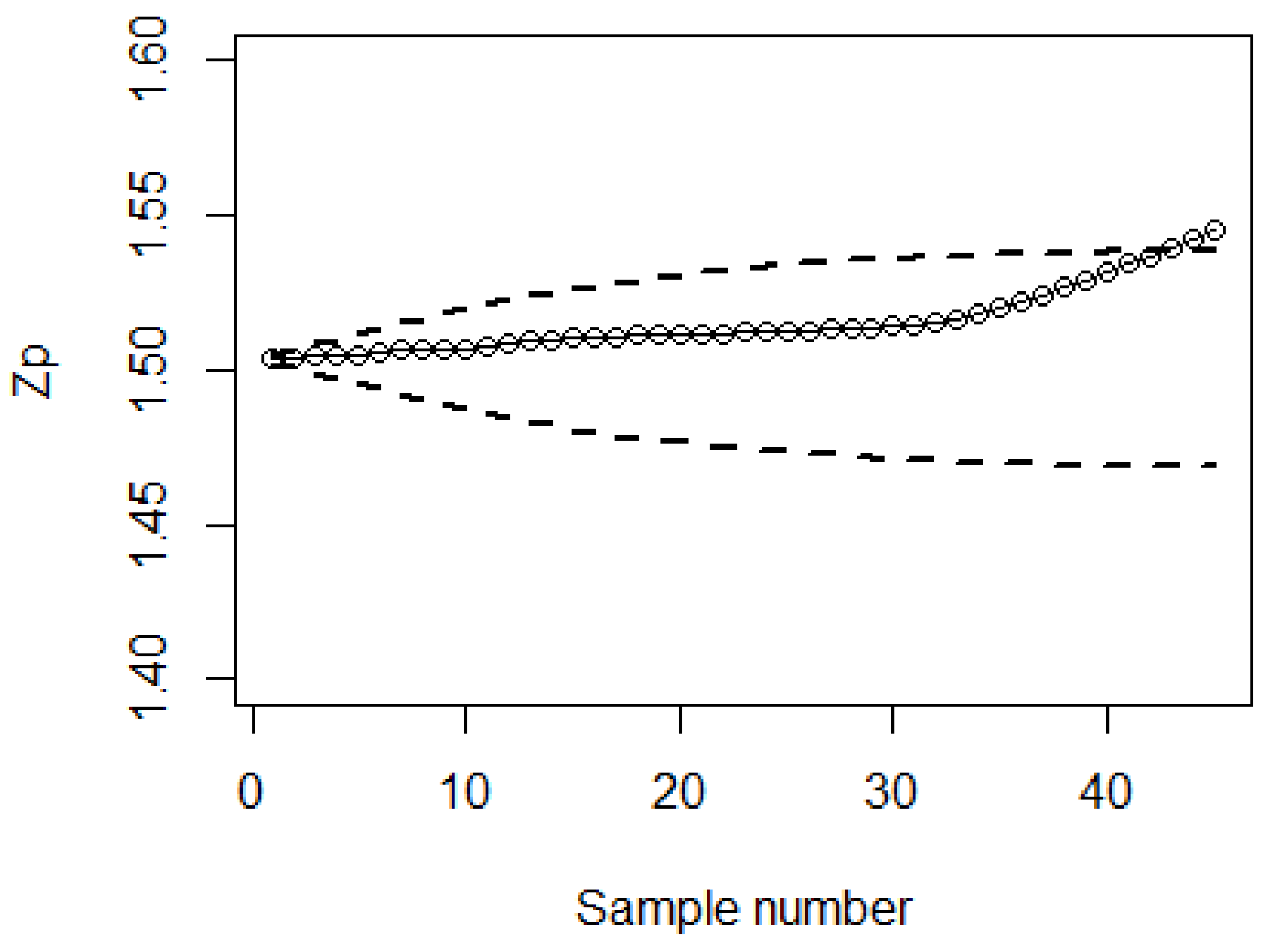
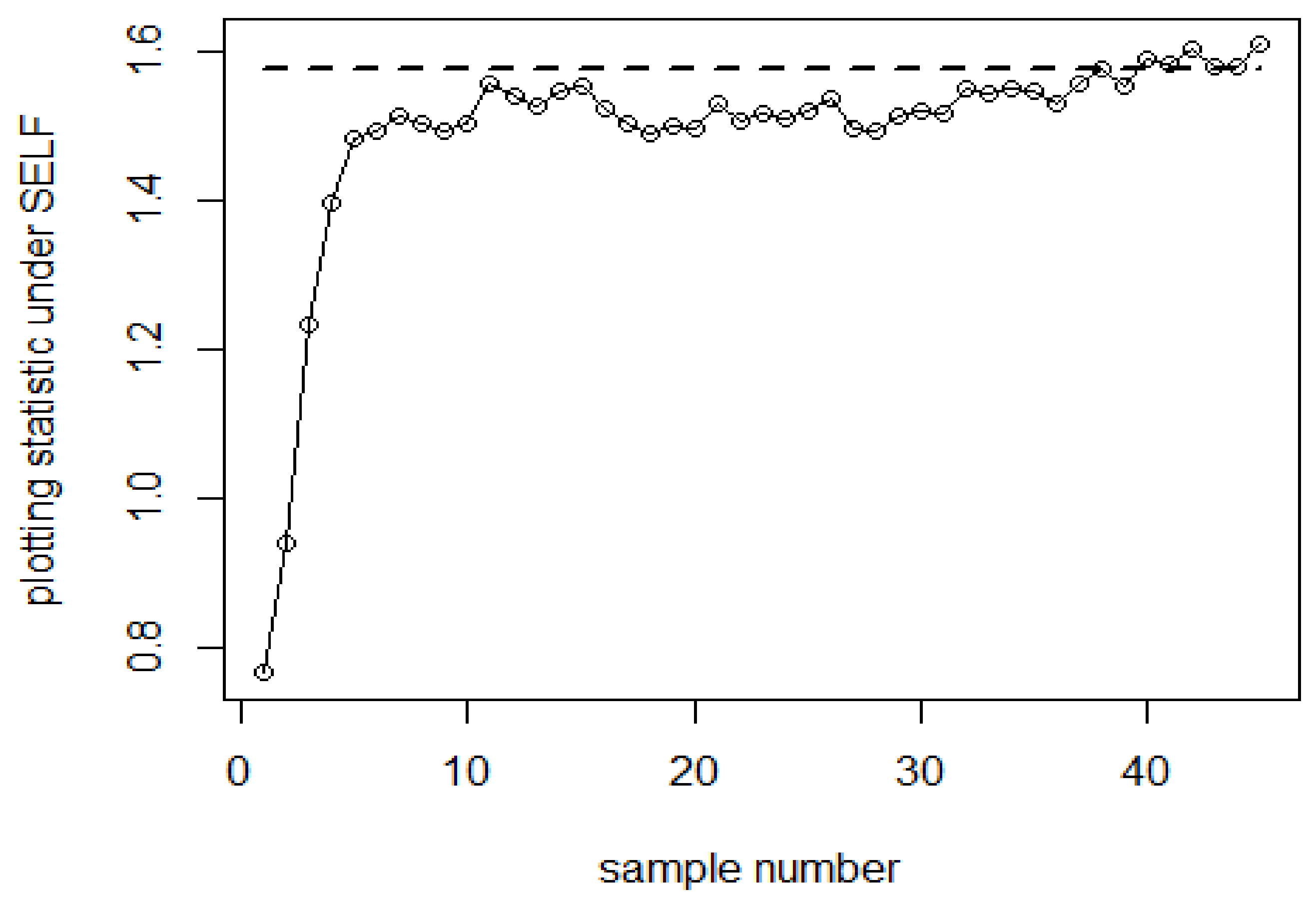
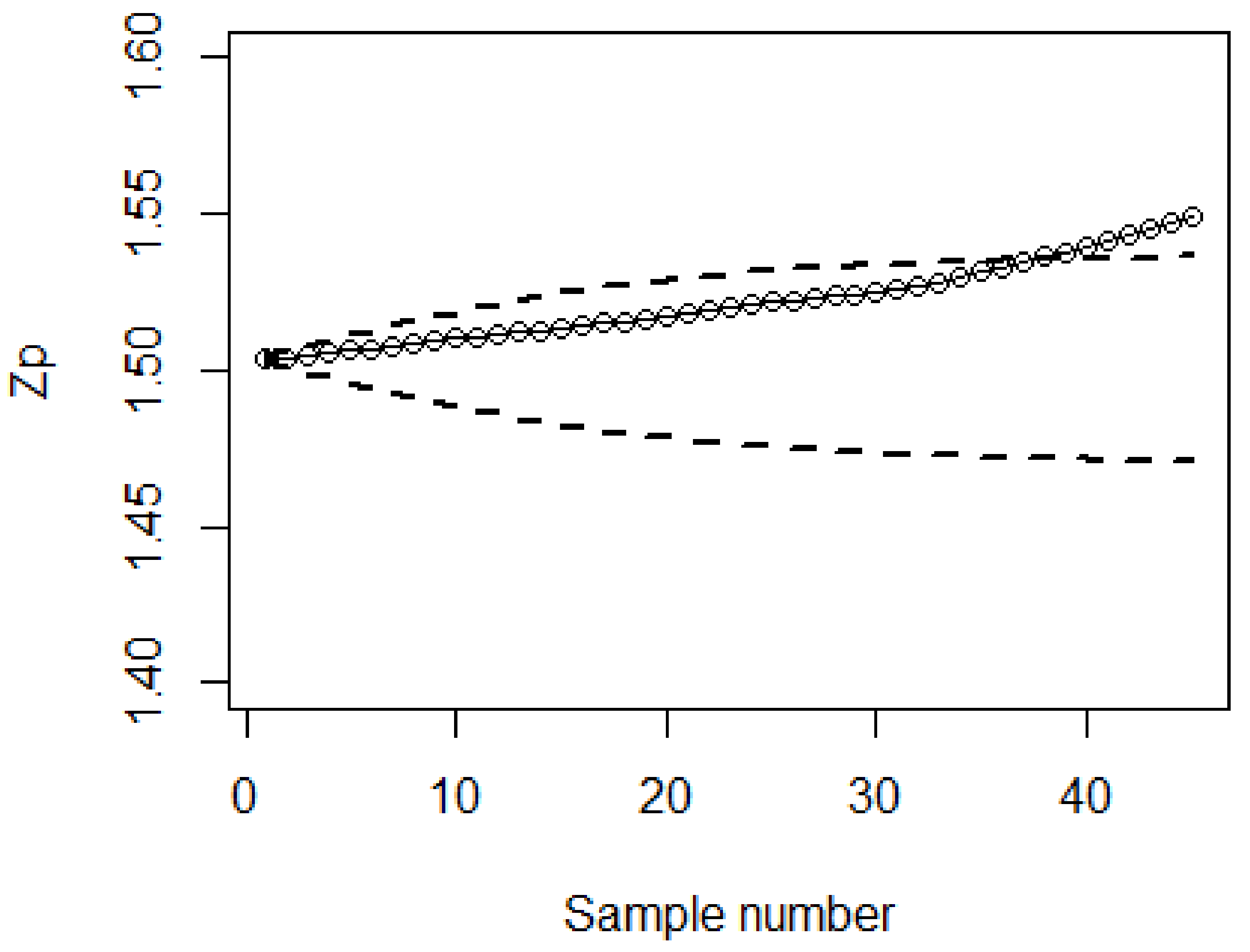
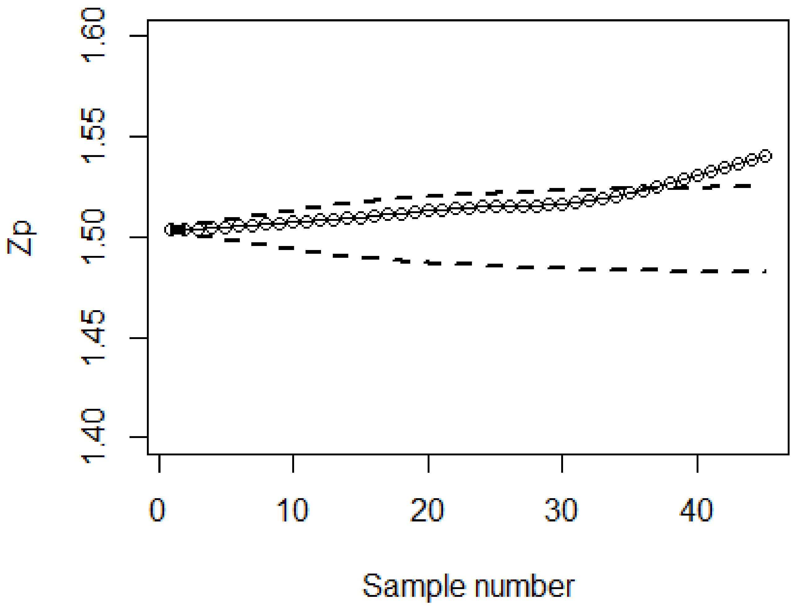
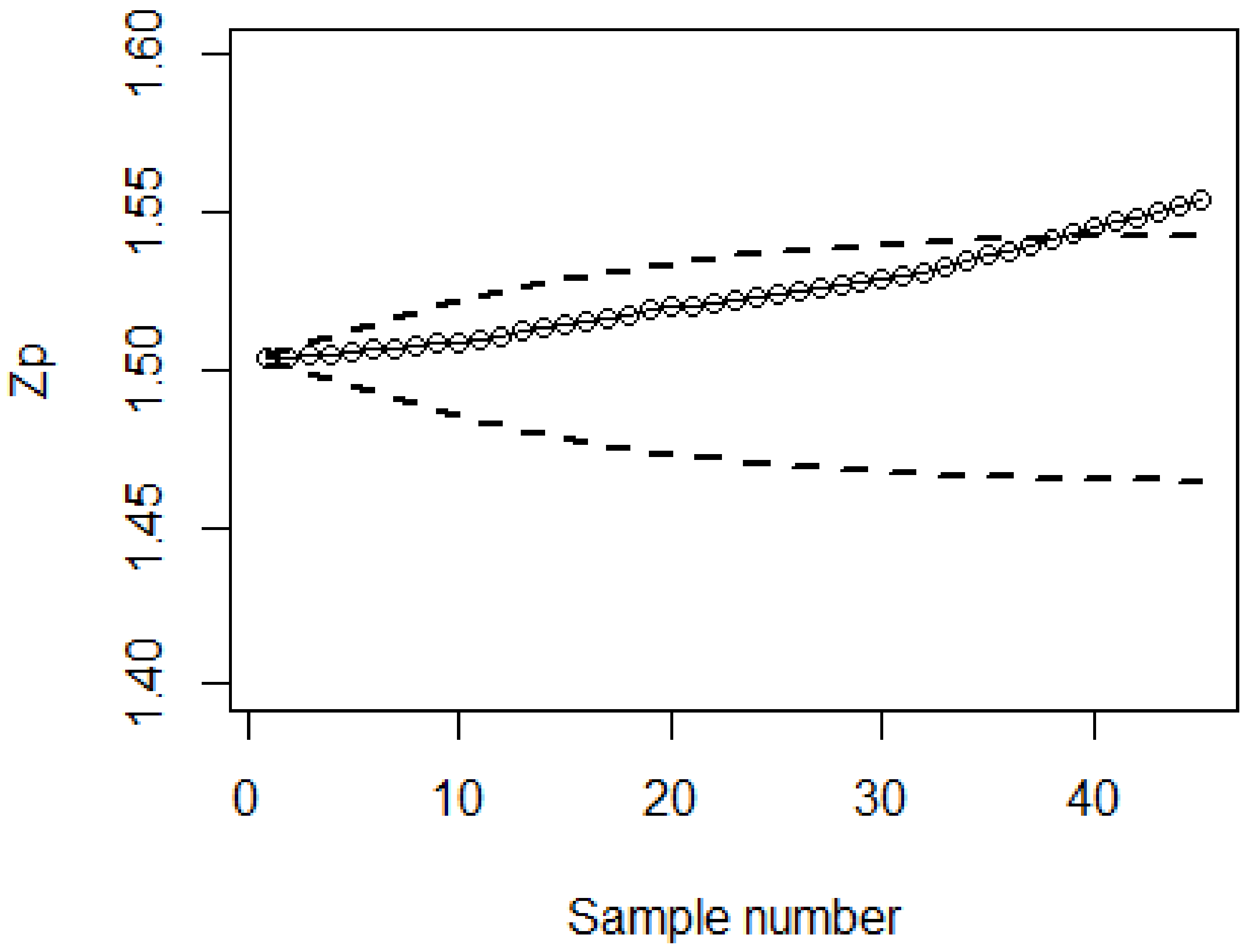
7. Real Data Applications

Inside the SPC literature, a standard exercise that has been used by many analysts is to clarify the execution and overall performance of the control charts using actual and simulated datasets. In this article, we use a real dataset to explain the work and execution of the proposed Bayesian AEWMA control chart under different RSS schemes utilizing two different LFs for posterior and posterior predictive distribution. The dataset is taken from Montgomery [26], which includes 45 samples, each of size 5 wafers. In semiconductor manufacturing, conjunction with photolithography is used with the hard-bake process. For measurement of the flow width microns are used, and a one hour time interval is taken between the samples. Consider the initial 30 samples from the in-control process (phase-I), while the remaining 15 samples from the out-of-control process (phase-II). Moreover, all the observation in the phase-II dataset is obtained by adding 0.017, which shows an ascending shift in the core process mean.
The HEWMA and AEWMA control charts under the Bayesian approach based on SRS by using SELF for posterior and posterior predictive distribution are shown in Figure 1 and Figure 2, respectively, which indicates that the process is out-of-control on the 42nd and 40th samples, respectively. Figure 2, Figure 3 and Figure 4 show the proposed Bayesian HEWMA control chart using SELF based on RSS schemes for posterior and posterior predictive distribution, the process shows out-of-control signals on the 36th, 35th, and 37th sample for RSS, MRSS, and ERSS, respectively. Based on Figure 1, Figure 2, Figure 3, Figure 4 and Figure 5, the suggested Bayesian HEWMA control charts using RSS schemes are more sensitive in detecting out-of-control signals than the Bayesian HEWMA and Bayesian AEWMA control charts using SRS.

8. Conclusions

In this article, a new Bayesian HEWMA control chart using different RSS schemes based on the informative prior distribution and with two LFs has been proposed for the process mean of the posterior and posterior predictive distribution. The results given in Table 1, Table 2, Table 3, Table 4, Table 5 and Table 6 show the efficiency of the suggested Bayesian HEWMA control chart using RSS schemes over the Bayesian HEWMA and Bayesian AEWMA control chart using SRS. The performance of the suggested control chart is also evaluated through different figures, which shows that the proposed control chart is faster in detecting out-of-control signals than an existing control chart. The current study is extended for different sampling schemes, LFs, and also for non-normal distribution, i.e., Weibull distribution or exponential distribution, etc.

Author Contributions

Conceptualization, I.K. and D.M.K.; Data curation, H.M.A. and U.K.; Formal analysis, I.K. and M.N.-u.-A.; Funding acquisition, H.M.A. and Z.A.; Investigation, D.M.K. and U.K.; methodology, D.M.K. and I.K.; Project administration, D.M.K. and H.M.A.; Resources, M.N.-u.-A. and U.K.; Software, I.K. and M.N.-u.-A.; Supervision, D.M.K. and U.K.; validation, U.K. and Z.A.; Visualization, M.N.-u.-A., Z.A. and H.M.A.; Writing—original draft preparation, I.K. and M.N.-u.-A.; writing—review and editing, D.M.K. and H.M.A. All authors have read and agreed to the published version of the manuscript.

Funding

Princess Nourah bint Abdulrahman University Researchers Supporting Project number (PNURSP2023R 299), Princess Nourah bint Abdulrahman University, Riyadh, Saudi Arabia.

Institutional Review Board Statement

Not applicable.

Informed Consent Statement

Not applicable.

Data Availability Statement

The data presented in this study are available on request from the corresponding author.

Conflicts of Interest

The authors declare no conflict of interest.

References

  1. Shewhart, W.A. The application of statistics as an aid in maintaining quality of a manufactured product. J. Am. Stat. Assoc. 1925, 20, 546–548. [Google Scholar] [CrossRef]
  2. Page, E.S. Continuous inspection schemes. Biometrika 1954, 41, 100–115. [Google Scholar] [CrossRef]
  3. Roberts, S. Control chart tests based on geometric moving averages. Technometrics 1959, 42, 97–101. [Google Scholar] [CrossRef]
  4. Lu, C.-W.; Reynolds, M.R., Jr. EWMA control charts for monitoring the mean of autocorrelated processes. J. Qual. Technol. 1999, 31, 166–188. [Google Scholar] [CrossRef]
  5. Khoo, M.B. A moving average control chart for monitoring the fraction of non-conforming. Qual. Reliab. Eng. Int. 2004, 20, 617–635. [Google Scholar] [CrossRef]
  6. Khan, N.; Aslam, M.; Jun, C.H. Design of a control chart using a modified EWMA statistic. Qual. Reliab. Eng. Int. 2017, 33, 1095–1104. [Google Scholar] [CrossRef]
  7. Saghir, A.; Ahmad, L.; Aslam, M. Modified EWMA control chart for transformed gamma data. Commun. Stat. Simul. Comput. 2021, 50, 3046–3059. [Google Scholar] [CrossRef]
  8. Adeoti, O.A.; Koleoso, S.O. A hybrid homogeneously weighted moving average control chart for process monitoring. Qual. Reliab. Eng. Int. 2020, 36, 2170–2186. [Google Scholar] [CrossRef]
  9. Arslan, M.; Anwar, S.M.; Lone, S.A.; Rasheed, Z.; Khan, M.; Abbasi, S.A. Improved adaptive EWMA control chart for process location with applications in groundwater physicochemical parameters and glass manufacturing industry. PLoS ONE 2022, 17, e0272584. [Google Scholar] [CrossRef]
  10. Tsui, K.-L.; Woodall, W.H. Multivariate control charts based on loss functions. Seq. Anal. 1993, 12, 79–92. [Google Scholar] [CrossRef]
  11. Menzefricke, U. On the evaluation of control chart limits based on predictive distributions. Commun. Stat. Theory Methods 2002, 31, 1423–1440. [Google Scholar] [CrossRef]
  12. Menzefricke, U. Combined exponentially weighted moving average charts for the mean and variance based on the predictive distribution. Commun. Stat. Theory Methods 2013, 42, 4003–4016. [Google Scholar] [CrossRef]
  13. Wu, Z.; Tian, Y. Weighted-loss-function CUSUM chart for monitoring mean and variance of a production process. Int. J. Prod. Res. 2005, 43, 3027–3044. [Google Scholar] [CrossRef]
  14. Serel, D.A. Economic design of EWMA control charts based on loss function. Math. Comput. Model. 2009, 49, 745–759. [Google Scholar] [CrossRef] [Green Version]
  15. Riaz, S.; Riaz, M.; Nazeer, A.; Hussain, Z. On Bayesian EWMA control charts under different loss functions. Qual. Reliab. Eng. Int. 2017, 33, 2653–2665. [Google Scholar] [CrossRef]
  16. Noor, S.; Noor-ul-Amin, M.; Mohsin, M.; Ahmed, A. Hybrid exponentially weighted moving average control chart using Bayesian approach. Commun. Stat. Theory Methods 2020, 51, 3960–3984. [Google Scholar] [CrossRef]
  17. Tang, Y.; Tan, S.; Zhou, D. An Improved Failure Mode and Effects Analysis Method Using Belief Jensen–Shannon Divergence and Entropy Measure in the Evidence Theory. Arab. J. Sci. Eng. 2022, 1–14. [Google Scholar] [CrossRef]
  18. Lin, C.H.; Lu, M.C.; Yang, S.F.; Lee, M.Y. A Bayesian Control Chart for Monitoring Process Variance. Appl. Sci. 2021, 11, 2729. [Google Scholar] [CrossRef]
  19. Noor-ul-Amin, M.; Noor, S. An adaptive EWMA control chart for monitoring the process mean in Bayesian theory under different loss functions. Qual. Reliab. Eng. Int. 2021, 37, 804–819. [Google Scholar] [CrossRef]
  20. Jeffreys, H. An invariant form for the prior probability in estimation problems. Proc. R. Soc. Lond. Ser. A. Math. Phys. Sci. 1946, 186, 453–461. [Google Scholar]
  21. Gauss, C. Methods Moindres Carres Memoire sur la Combination des Observations; Bertrand, J., Translator; Nabu Press: Charleston, SC, USA, 1955. [Google Scholar]
  22. Varian, H.R. A Bayesian approach to real estate assessment. In Studies in Bayesian Econometrics and Statistics: In Honor of L. J. Savage; North-Holland Pub. Co.: Amsterdam, The Netherlands, 1975; pp. 195–208. [Google Scholar]
  23. McIntyre, G. A method for unbiased selective sampling, using ranked sets. Aust. J. Agric. Res. 1952, 3, 385–390. [Google Scholar] [CrossRef]
  24. Muttlak, H. Median ranked set sampling. J. Appl. Stat. Sci. 1997, 6, 245–255. [Google Scholar]
  25. Samawi, H.M.; Ahmed, M.S.; Abu-Dayyeh, W. Estimating the population mean using extreme ranked set sampling. Biometr. J. 1996, 38, 577–586. [Google Scholar] [CrossRef]
  26. Montgomery, D.C. Introduction to Statistical Quality Control; John Wiley & Sons: Hoboken, NJ, USA, 2007. [Google Scholar]
Figure 1. Bayesian HEWMA control chart using posterior and posterior predictive distribution under SELF for SRS.
Applsci 13 02837 g001
Figure 2. Bayesian AEWMA control chart using posterior and posterior predictive distribution under SELF for SRS.
Applsci 13 02837 g002
Figure 3. Bayesian HEWMA control chart using posterior and posterior predictive distribution under SELF for RSS.
Applsci 13 02837 g003
Figure 4. Bayesian HEWMA control chart using posterior and posterior predictive distribution under SELF for MRSS.
Applsci 13 02837 g004
Figure 5. Bayesian HEWMA control chart using posterior and posterior predictive distribution under SELF for ERSS.
Applsci 13 02837 g005
Table 1. The ARL and SDRL values of Bayesian HEWMA and Bayesian AEWMA control charts for posterior and posterior predictive distribution under SELF, for λ 1 = 0.10 and λ 2 = 0.05, n = 5.
ShiftBayesian HEWMA SRSBayesian
AEWMA SRS
Bayesian HEWMA RSSBayesian
HEWMA MRSS
Bayesian
HEWMA ERSS
ARLSDRLARLSDRLARLSDRLARLSDRLARLSDRL
L = 2.099h = 0.0856L = 2.085L = 2.081L = 2.0864
0.00371.67408.54370.86537.77370.17409.83368.36425.51371.51423.98
0.10196.95205.05179.91247.52108.18104.5692.7591.5092.21114.53
0.2082.9380.7270.6191.1229.4027.8027.4924.3141.7736.00
0.3045.2840.1935.4044.5319.7315.6716.6713.3822.0417.86
0.4028.2523.6421.1526.3612.419.5310.478.0513.8810.71
0.5019.7715.9213.5516.698.516.557.045.309.507.24
0.6014.7011.439.4611.236.144.595.193.817.135.40
0.7011.558.907.087.704.903.593.982.885.474.07
0.7510.167.846.156.434.243.063.592.574.843.63
0.809.086.865.625.823.802.733.202.214.343.16
0.907.505.654.514.183.152.222.681.793.512.53
1.006.334.753.853.202.641.812.191.422.962.05
1.503.192.252.251.291.470.761.290.571.610.88
2.001.981.231.660.781.110.341.050.231.170.42
2.501.460.751.360.561.020.14101.030.19
3.001.210.471.170.39101010
4.001.020.161.010.14101010
Table 2. The ARL and SDRL values of Bayesian HEWMA and Bayesian AEWMA control chart for posterior and posterior predictive distribution under SELF, for λ 1 = 0.25 and λ 2 = 0.05. n = 5.
ShiftBayesian HEWMA SRSBayesian
AEWMA SRS
Bayesian HEWMA RSSBayesian
HEWMA MRSS
Bayesian
HEWMA ERSS
ARLSDRLARLSDRLARLARLSDRLARLSDRLARL
L = 2.2709h = 0.241L = 2.2656L = 2.2644L = 2.2654
0.00370.10389.87369.00367.39369.48390.26371.03375.35369.48424.80
0.10205.54213.07210.23195.27109.64104.51101.6797.65109.65107.20
0.2089.6385.7597.0480.9138.8733.8628.9025.8432.7731.97
0.3048.0842.6455.7142.8020.4215.9417.1613.2523.4318.51
0.4030.2824.8836.1525.0913.109.6510.757.6514.4910.78
0.5020.8416.4125.9517.048.976.467.415.2510.067.19
0.6015.4211.6519.8012.206.544.545.413.727.465.24
0.7012.008.8015.419.095.183.554.212.835.764.00
0.7510.677.7314.118.174.523.053.802.495.143.56
0.809.546.9212.877.264.132.783.402.234.643.16
0.907.945.6510.765.973.412.222.801.783.812.52
1.006.604.639.174.962.841.792.391.473.182.06
1.503.412.224.902.771.560.801.360.611.710.93
2.002.141.272.981.831.140.381.080.281.210.47
2.501.560.811.981.151.020.16101.050.22
3.001.260.521.480.72101010
4.001.040.2010101010
Table 3. The ARL and SDRL values of Bayesian HEWMA and Bayesian AEWMA control chart for posterior distribution using under LLF, for λ 1 = 0.10 and λ 2 = 0.05, n = 5.
ShiftBayesian HEWMA SRSBayesian
AEWMA SRS
Bayesian
HEWMA RSS
Bayesian
HEWMA MRSS
Bayesian
HEWMA ERSS
ARLSDRLARLSDRLARLARLSDRLARLSDRLARL
L = 2.096h = 0.086L = 2.092L = 2.095L = 2.097
0.00369.17401.10370.98539.06369.74411.30370.48401.71371.46407.25
0.10195.13204.24184.38254.91108.54111.6892.7693.98117.72116.86
0.2084.7982.1771.9892.4838.1233.3128.9325.6229.7829.10
0.3045.1340.3636.2645.4919.9115.9516.3613.0122.0617.88
0.4028.2223.5121.0926.3012.469.6910.147.8113.8910.78
0.5019.7815.9613.7116.738.486.406.955.289.707.42
0.6014.6711.449.5311.256.214.675.153.817.025.33
0.7011.288.667.097.864.833.563.962.845.404.06
0.7510.077.776.206.504.333.193.522.494.833.54
0.809.236.975.545.543.832.773.182.264.313.13
0.907.495.674.524.173.192.242.611.753.542.51
1.006.234.653.833.202.641.792.201.432.972.09
1.503.152.212.261.271.470.751.280.561.610.91
2.001.981.231.660.781.110.341.050.231.170.43
2.501.460.751.340.551.010.13101.030.19
3.001.210.471.160.39101010
4.001.020.161.020.15101010
Table 4. The ARL and SDRL values of Bayesian HEWMA and Bayesian AEWMA control chart for posterior distribution using under LLF, for λ 1 = 0.25 and λ 2 = 0.05, n =5.
ShiftBayesian HEWMA SRSBayesian
AEWMA SRS
Bayesian
HEWMA RSS
Bayesian
HEWMA MRSS
Bayesian
HEWMA ERSS
ARLSDRLARLSDRLARLARLSDRLARLSDRLARL
L = 2.2716h = 0.242L = 2.2777L = 2.2644L = 2.2785
0.00371.51399.34370.14434.88370.33413.48371.31402.39369.64455.17
0.10204.28211.60212.09198.42122.91129.19102.44104.20131.00127.63
0.2091.1787.08 86.7783.2532.0830.0933.9528.4033.7528.30
0.3048.5442.9855.4442.2620.7015.9817.4513.2624.0118.96
0.4030.3224.9236.7625.9813.009.7510.797.8714.6811.01
0.5020.1016.2425.8616.888.846.307.435.3110.107.31
0.6015.3211.4419.6512.166.714.715.533.747.545.24
0.7011.888.7115.629.175.153.524.222.835.803.97
0.7510.677.6914.238.294.563.113.832.525.193.56
0.809.646.9012.837.304.112.773.412.214.693.17
0.907.835.5910.795.903.392.222.841.813.872.56
1.006.674.629.255.002.871.822.391.463.212.09
1.503.392.234.952.801.570.821.360.621.730.95
2.002.151.292.971.811.150.391.070.261.230.49
2.501.560.801.971.131.020.16101.050.23
3.001.260.521.480.73101010
4.001.040.201.090.30101010
Table 5. The ARL and SDRL values of Bayesian HEWMA and Bayesian AEWMA control chart for posterior predictive distribution using under LLF, for λ 1 = 0.10 and λ 2 = 0.05, n = 5.
ShiftBayesian HEWMA SRSBayesian
AEWMA SRS
Bayesian
HEWMA RSS
Bayesian
HEWMA MRSS
Bayesian
HEWMA ERSS
ARLSDRLARLSDRLARLSDRLARLSDRLARLSDRL
L = 2.097h = 0.0856L = 2.096L = 2.093L = 2.092
0.00371.01407.30369.58524.70370.91386.10371.20425.62369.87381.21
0.10196.48206.11178.57250.19114.59118.4192.1889.24122.70125.56
0.2085.4482.9170.5391.2237.3832.2525.1524.8740.7637.20
0.3045.5240.2735.7145.2520.0715.9716.1812.7422.1117.96
0.4028.5723.8321.2426.2912.489.5910.327.8814.0210.95
0.5019.6515.6413.6616.908.386.356.915.219.467.28
0.6014.8111.559.4611.086.274.795.123.777.035.37
0.7011.388.826.947.704.863.573.952.885.434.01
0.7510.197.826.226.534.283.163.552.544.863.58
0.809.176.965.505.583.822.773.202.264.333.20
0.907.535.664.524.153.152.202.581.763.552.50
1.006.284.743.773.172.651.792.201.422.972.07
1.503.132.192.261.291.470.761.280.561.620.90
2.001.971.211.660.781.110.341.030.161.170.43
2.501.460.751.350.551.020.14101.030.19
3.001.210.471.160.39101010
4.001.020.171.020.15101010
Table 6. The ARL and SDRL values of Bayesian HEWMA and Bayesian AEWMA control chart for posterior predictive distribution under LLF, for λ 1 = 0.25 and λ 2 = 0.05, n = 5.
ShiftBayesian HEWMA SRSBayesian
AEWMA SRS
Bayesian
HEWMA RSS
Bayesian
HEWMA MRSS
Bayesian
HEWMA ERSS
ARLSDRLARLSDRLARLSDRLARLSDRLARLSDRL
L = 2.2717h = 0.2414L = 2.2771L = 2.2649L = 2.2781
0.00372.35391.96368.67359.45380.12396.83369.24386.76368.89436.27
0.10206.32211.24210.29197.72112.72122.32100.7099.31130.03128.34
0.2090.3086.0198.1683.2440.6134.9233.6128.4046.0140.51
0.3048.0742.8654.9241.4520.8916.3616.8312.7923.2818.24
0.4030.5425.3036.1925.4813.049.6810.757.8414.5710.91
0.5020.7716.2825.9717.138.986.427.315.2110.207.32
0.6015.3911.5119.6812.216.644.595.463.757.475.22
0.7011.948.7315.569.195.123.494.212.855.824.03
0.7510.687.7214.188.264.613.123.732.515.213.57
0.809.586.7812.797.244.132.783.342.194.653.15
0.907.835.5310.745.933.412.232.801.783.822.53
1.006.654.679.204.982.881.822.321.433.222.09
1.503.352.214.942.791.580.821.360.621.710.91
2.002.161.282.951.811.140.381.070.261.230.48
2.501.560.801.981.141.020.17101.050.23
3.001.260.521.480.72101010
4.001.040.201.090.30101010
Disclaimer/Publisher’s Note: The statements, opinions and data contained in all publications are solely those of the individual author(s) and contributor(s) and not of MDPI and/or the editor(s). MDPI and/or the editor(s) disclaim responsibility for any injury to people or property resulting from any ideas, methods, instructions or products referred to in the content.

