Abstract
In this article we present a space–time epidemic-type aftershock sequence (ETAS) model for the area of Hungary, motivated by the goal of its application in insurance risk models. High-quality recent instrumental data from the period 1996–2021 are used for model parameterization, including data from the recent nearby Zagreb and Petrinja event sequences. In the earthquake-triggering equations of our ETAS model, we replace the commonly used modified Omori law with the more recently proposed stretched exponential time response form, and a Gaussian space response function is applied with a variance add-on for epicenter error. After this model was tested against the observations, an appropriate overall fit for magnitudes was found, which is sufficient for insurance applications, although the tests also show deviations at the threshold. Since the data used for parameterization are dominated by Croatian earthquake sequences, we also downscale the model to regional zones via parameter adjustments. In the downscaling older historical data are incorporated for a better representation of the key events within Hungary itself. Comparison of long-term large event numbers in simulated catalogues versus historical data shows that the model fit by zone is improved by the downscaling.
1. Introduction
1.1. Motivation
The origin of the study presented in this article is an ongoing effort by the UNIQA Insurance Group (www.uniqagroup.com, accessed on 5 February 2023) to build a proprietary earthquake model for Hungary. Earthquake models in insurance are used to measure the risk of a set of objects, such as buildings, civil engineering structures, and means of transport, with a focus on assessing the potential losses caused by severe earthquakes.
One key application of an earthquake model or, more generally, a natural catastrophe model in insurance is the determination of capital requirements. According to the Solvency II regulatory standards applicable in European Union member countries [1,2], the solvency capital requirement (SCR) of an insurance company shall correspond to the 200-year loss; that is, the insurer must hold their own funds to cover the risk of a loss whose probability of occurrence within a year is 0.5%. The SCR is calculated either by the Solvency II standard formula or by an internal model. For natural perils, the standard formula is a deterministic approximation of the risk based on fixed factors applied to insured amounts of the objects by geographical area. On the other hand, an internal model is based on the stochastic simulation of the peril, and its output is not just an SCR single value but a full probability distribution forecast of the loss. The use of an internal model by an insurance company for calculating the SCR is subject to case-by-case regulatory approval by the competent supervisory authorities, including a comprehensive and lengthy validation process. The development of an internal model requires a significant effort; however, the benefits include a more accurate and more detailed evaluation of the risk, and a range of model uses in risk management tasks beyond the calculation of the SCR. Another typical and important use of stochastic catastrophe models is the optimization and pricing of protection covers for the purpose of risk transfer. Reinsurance risk transfer is an instrument for risk mitigation, and it can reduce the SCR of the ceding insurer.
The general architecture of a stochastic earthquake model for insurance is the following: (1) the first fundamental module is a statistical model of earthquake occurrences, which is used to generate a synthetic event catalogue via stochastic simulation. This is followed by two equally important ones: (2) the ground motion attenuation model, translating the catalogue into event footprints, and (3) the vulnerability model, translating the event footprints into the loss of the insured objects in financial terms. All three modules require a full study of their own. In this article, only the first module is discussed, that is, a model of earthquake occurrences.
Earthquake models used in the field of insurance typically focus on the mainshocks only. This simplifies the modelling effort drastically since the mainshocks are assumed to follow a stationary process. This simplification is justified if aftershock losses are low compared to the mainshock loss. Furthermore, customer claims arising from aftershock losses are often not reported separately from the mainshock; therefore, it is a straightforward approach to model them only implicitly via conservative parameterization. Nevertheless, the recent nearby Petrinja 2020 event in Croatia and its aftershocks highlighted some properties of earthquake sequences [3], suggesting that clustering cannot necessarily be safely ignored even in a Central European model: aftershock activity after such a major event may last for months or even years, and some aftershocks (or foreshocks) are significant events on their own. Moreover, there are historical records of complex earthquake sequences (e.g., Romania 1991) lasting for several months and including multiple significant shocks [4]. Large events are still possible late in the sequence, and large aftershocks can trigger second-generation sequences, epidemic style.
1.2. Aim of the Study
The aim of this study is to build an epidemic-type aftershock sequence (ETAS) model for Hungary using recent instrumental earthquake catalogue data. ETAS methodology assumes that, on top of a constant background seismicity, every single earthquake is a potential trigger for subsequent events. Such models have been widely used to analyse earthquake clustering both for studies covering broad regions and local studies focusing on individual earthquake sequences. This study builds on existing methodologies, however, the planned implementation for insurance application is always considered in the choice of the methods.
Due to its moderate seismicity, Hungary is not an optimal target area for an ETAS model. Nonetheless, the nearby Zagreb and Petrinja event sequences in 2020–2021 produced rich data that make the parameter fitting feasible. The authors do not know about a published previous region-specific ETAS study for Hungary relying on these recent catalogue data; therefore, the results can be interesting themselves.
The data used in the study are described in Section 2. In Section 3, an overall model for Hungary is formulated and in Section 4, its results are described. In Section 5 and Section 6, downscaled parameters are determined, representing local regions within the total modelled area. The motivation of parameter downscaling stems from the application of the model in insurance where local geographical outputs are needed. Section 7 includes the conclusions of the study.
1.3. Background
Since the initial formulation of the model by Ogata [5,6], ETAS methodology has been researched extensively. Works by several authors suggested different methods and algorithms for parameter estimation [6,7,8,9,10] and investigated the optimal forms of event-triggering functions [6,8,11,12]. The literature on ETAS also includes a discussion of important model properties. One such model property is magnitude independence, i.e., the assumption that the magnitude of an earthquake is independent of predecessor events [8,13]. The stability or criticality conditions of the event triggering, as well as the question of self-similarity, have been investigated [14,15]. Certain enhancements of the model that allow a more accurate modelling of complex processes, such as three-dimensional or finite-source ETAS models, have also been developed [9,16,17]; however, the benefits of these advanced features for modelling a moderately active region like Hungary are not immediately clear.
This study significantly relies on the work of Zhuang et al. [7,8], who developed an iterative algorithm for ETAS parameterization, based on a kernel density estimation of the background activity in combination with stochastic declustering. The authors analyse the properties of the method in regional studies covering areas of Japan and New Zealand, and they suggest a range of methods for testing the different components of the model.
ETAS parameter estimation is affected by known sensitivities and biases, which are discussed at length by Seif et al. [18], who demonstrate these effects on actual and simulated catalogues derived from Italian and South Californian data. Typical sources of parameter bias include early aftershock incompleteness in the wake of a major earthquake, the anisotropy of aftershock clusters, and the choice of the magnitude threshold. These effects also need to be considered in this Hungarian study.
2. Data
The data quality requirements of an ETAS model fitting are challenging. A consistent instrumental earthquake catalogue for Hungary and the seismograph network collecting the measurements for this catalogue have only been in place since 1996 [19], and there has been a scarcity of significant Hungarian events from 1996 until 2022. For a sufficiently rich catalogue, the 2020 Zagreband the 2020 Petrinja, Croatia events and their aftershock sequences need to be included in the study. It is relevant to note that the Petrinja mainshock also caused damage and triggered insurance claims within Hungary [20]. These two event sequences have been recorded by the Hungarian seismograph network. On the other hand, both clusters fell largely outside the core geographical window of the Hungarian earthquake catalogue; this means that the study area is extended to the periphery of the data sources where the completeness and accuracy of data is less than optimal. Furthermore, large Croatian event sequences will have a dominant effect on the model fitting.
The core geographical window of the study is the area between latitudes 45.5–49.0 N and longitudes 16.0–23.0 E. In order to include the Zagreb and Petrinja events, a margin to the west and to the south is added by defining the extended window as the area between latitudes 45.3–49.0 N and longitudes 15.7–23.0 E. The magnitude threshold of the study is set at .
The data available for the study include both historical and recent instrumental data belonging to several Hungarian earthquake catalogues. These catalogues have been merged and event magnitudes have been homogenized to moment magnitude for this study. Hereafter, the subscript is omitted when referring to magnitudes. The component catalogues are the following (see also Figure 1):
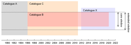
Figure 1.
Schematic diagram of the coverage and overlaps of the source catalogues used in the study.
- Catalogue A: Historical catalogue for the period 456 A.D. to 1995 [21], collected from several primary sources, partly instrumental and partly macroseismic. The number of events included in the extended window that reach the magnitude threshold is 2402. Due to obvious data quality limitations, these events are not used directly for ETAS parameter fitting but only as data for subsequent model downscaling.
- Catalogue B: Instrumental catalogue covering the core window and the period 1996 to 2019, based on the recordings of the Hungarian seismograph network [19]. The number of events reaching the magnitude threshold is 654.
- Catalogue C: Instrumental catalogue data for the period 1996 to 2010, collected and merged from international sources [22,23,24]. While some of the underlying sources are continuously updated, the merged dataset is only available to the end of 2010. The number of events included in the extended window that reach the magnitude threshold is 1107, partly overlapping with catalogue B data in the core window.
- Catalogue X: Initial event list (IEL) data covering the period 2012 to 2021 [25], based on the recordings of the Hungarian seismograph network. IEL data are an interim phase of the yearly updates of the Hungarian instrumental earthquake catalogue (catalogue B). Geographical coverage is wider than the core window by a margin of 0.2 degrees latitude and 0.3 degrees longitude in all directions. Automated preliminary epicenter determinations are post-processed for the monthly publications of the list, which may result in some coordinate shifts across the window boundary. Thus, the western and southern edge of the extended window corresponds approximately to the geographical scope of the IEL. The number of events from IEL included in the extended window that reach the magnitude threshold is 2313, fully overlapping with catalogue B data in the core window in the period 2012 to 2019.
Microseismic events caused by quarry blasts and explosions had been identified and excluded from the datasets during the preparation of the catalogues prior to this study.
It is observed that the events in the Romanian area of the study show unusual magnitude–frequency patterns. This suggests an inhomogeneity of the merger of the primary sources underlying the Romanian part of catalogue C. Therefore, the affected area is excluded from the ETAS parameter fitting due to concerns of data quality. The boundary of the excluded area follows the area source zone boundaries of the SHARE project [26]. Therefore, the exclusion affects a strip within Hungary along the Romanian border.
Magnitude–frequency distributions suggest that the completeness threshold of the remaining catalogue on the core window is at the beginning in 1996, which has gradually improved to by 2000 and to by 2013. The sensitivity contours of the Hungarian seismograph network indicate completeness for on most of the modelled area in the core window with some lower-sensitivity areas on the periphery and with gradually improving coverage over time [19]. The catalogue is considered complete for in the extended window only since 2018, except for a completeness gap immediately after the Petrinja 2020 mainshock: the detection of early aftershocks after a large earthquake is typically incomplete since the seismograms in this initial period are saturated with overlapping waves from multiple events [18]. Given the trade-off between completeness and the size of the catalogue, we find that the optimal choice of the threshold for this study is . A threshold increase would marginalize the part of the catalogue within Hungary itself and would sharply reduce the number of events for estimating the spatial distribution of the background process. For the model parameterization, completeness is assumed on the core window since 2000 and on the extended window since 2018, except for a 1-day period after the Petrinja mainshock.
After merging catalogues B, C, and X, applying the threshold, removing duplications, removing events outside the completeness periods, and removing events in the excluded area, the remaining size of the target catalogue for ETAS parameter fitting is 1978. An additional 236 events reaching are used as auxiliary trigger events; this includes 27 events from year 1999 and 209 events from the Petrinja completeness gap. A map of the fitting catalogue is shown in Figure 2. Another 218 events from catalogues B, C, and X outside the completeness periods are used as additional epicenter nodes for the kernel density estimation of the spatial distribution of background events.
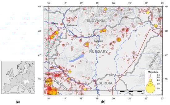
Figure 2.
(a) Location of the model area within Europe. (b) Plot of the earthquake catalogue for Hungary used for epidemic-type aftershock sequence (ETAS) model parameterization—target catalogue plus auxiliary events, 1999–2021. The map covers the extended window. The boundaries of the core window (dashed black line) and excluded area (red line) are marked. Events reaching are highlighted.
For model calculations, geographical latitude–longitude coordinates are converted to an kilometre grid via the following transformation:
where is the mean radius of the Earth in kilometres. This corresponds to a tangent transverse cylindrical projection whose central meridian is at and that transforms parallels into straight lines. The point is set at (47.5°, 19°), i.e., the rounded coordinates of Budapest, which are transformed into in the kilometre grid.
3. Epidemic-Type Aftershock Sequence (ETAS) Modelling Methods
3.1. Model Formulation
The ETAS model describes earthquake occurrences as a non-stationary Poisson point process where every event can trigger a wave of aftershocks. In a time-only model, the rate of occurrence at time , conditional on the process history , is expressed as [5]
which is extended to a space–time model as [6]
where the first term represents background seismicity with a constant overall rate and area density , and the sum in the second term reflects the rate of activity triggered by events in the catalogue prior to time . An exponential relationship is assumed between the trigger event magnitude and the triggered rate of activity, where and are constant parameters and is the magnitude threshold. The functions and describe the form of the time and space response, respectively, relative to the trigger event occurrence time and epicenter. The process history is the catalogue of events before , defined by their occurrence time, location, and magnitude. Depth is not included in this ETAS model as a third coordinate, and the question of the depth distribution is not discussed in this article. This is a reasonable simplification since all events in the study catalogue were shallow crustal earthquakes and all except nine of them had a focal depth of less than 20 km.
It was assumed that event magnitudes follow a truncated exponential (Gutenberg-Richter) distribution independent of the process history [8,13]. The probability density function (PDF) of magnitudes between the bounds and is given by the following:
where is the frequency decay parameter. According to the magnitude independence assumption, an aftershock can be larger than its trigger event.
For this study, we used a stretched exponential function truncated for a minimum delay as the time response:
where is a minimum delay parameter, and the normal distribution with an allowance for epicenter error is the space response function:
where is the scale parameter of the magnitude-dependent part of the variance, and is a parameter representing a variance add-on for epicenter error. Since both Equation (5) and Equation (6) represent a departure from the mainstream techniques, we explain the rationale of these approaches below.
The most often used time response function is the modified Omori law [27], which is a power law function in the form of . The stretched exponential alternative has been suggested by Mignan [12], who, besides quantitative tests showing that the stretched exponential form is better fitted to the observations from several regions than the power law, also expressed qualitative concerns about the modified Omori law. Firstly, the positive time shift constant avoids the singularity at zero, but it is difficult to find a physical explanation for it. Secondly, a parameter value of would mean an infinite number of triggered events unless the process is artificially truncated in time. Furthermore, due to the heavy tail of the power law function, supercritical parameter fitting outcomes, which imply an unstable process, are sometimes obtained when the modified Omori law is used in an epidemic-type model [18]. The minimum delay parameter in Equation (5) is motivated by experience with stochastic simulations based on the model. This truncation was introduced to avoid modelling an unrealistically high number of aftershocks immediately after the trigger event, which were never observed or identified as separate events in actual measurements since the point process model reaches its limits at very short time intervals.
Regarding the space response function, observed aftershock sequences often show anisotropic patterns. Nonetheless, isotropic functions are widely used in ETAS models as a simplification. Both the power law function, e.g., in the form and the bivariate normal distribution have been discussed in the literature with a general preference for the power law based on goodness-of-fit diagnostics [6,8]. The Gaussian form is chosen in this study mainly for its analytical simplicity and ease of implementation in the model. Since the exponential scaling parameter is the same in Equations (3) and (6), the space response formula assumes that the aftershock area grows in proportion to the number of events triggered, which is in line with the observed trend known as the Utsu–Seki law [6,27]. This constraint from early ETAS model variants has been challenged in the literature, raising the suggestion for a separate spatial scaling parameter [8,11]. However, due to the small number of major clusters available in the Hungarian catalogue, it is preferred to keep the number of fitted parameters as low as possible. Finally, for the moderately strong Hungarian events in the study period, a weak spatial scaling trend between trigger event magnitudes and aftershock radii is observed. It is assumed that the underlying effect is the epicenter error, which becomes a dominant factor at low magnitudes; hence, the motivation to include the parameter. We note that the formulation in Equation (6) is a simplified reflection of epicenter error when the space response function is centred on the observed epicenters rather than the underlying ones. In a precise mathematical model, the conditional distributions of the error vectors would be neither isotropic nor independent.
When an isotropic space–time model is fitted to non-isotropic aftershock data, a typical impact is a downward bias of the parameter; an indication of this effect is a significant gap between the values estimated from space–time versus time-only models [18,28]. This effect is avoided by applying the constraint , motivated by the assumption of self-similarity: when the magnitude threshold of the model is shifted from to , the parameter is rescaled to while ignoring the upper magnitude bound for simplicity; therefore, the model parameters are almost unchanged across magnitude scales if except in the vicinity of the upper bound . Such a model also preserves Båth’s law, i.e., the observation that the average magnitude difference between a trigger event and its biggest aftershock appears to be invariant [9,14,18] (S1.2.1) [29].
The branching ratio of the model characterizing the stability of the process is defined as the average number of the first-generation descendants triggered by an event and expressed as [8,18]:
The process is subcritical (stable) if , it is critical (unstable) if , and it is supercritical (unstable, potentially explosive) if . In a model describing earthquake recurrence over extended periods, subcritical behaviour is assumed. Therefore, assuming a self-similar process with and substituting Equations (4) and (5) in Equation (7), the branching ratio is:
which considers the truncation of the time response function at . There is a near-linear dependence of on the magnitude span , where the upper bound is difficult to estimate and the lower bound is subject to expert judgement. Therefore, the branching ratio according to Equations (7) and (8) is better viewed as a model property rather than as a physical parameter of the observed earthquake catalogue.
3.2. Parameter Fitting
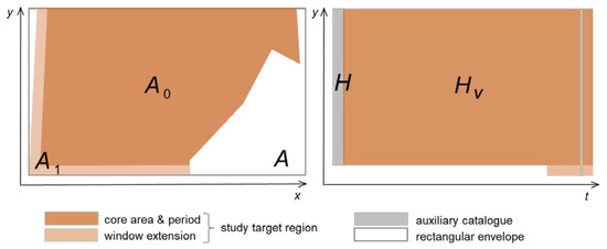
In this subsection the parameter fitting process for a space–time ETAS model formulated in Equations (3)–(6) is described. The study period is with where time is measured in days beginning at 2000-01-01 00:00 UTC. The broader study area is , where space coordinates follow the kilometre grid defined in Equation (1). The core study area and the proper study area are narrower than , so (see Figure 2 and Figure 3). The lower and upper magnitude bounds are set at and , respectively; it is assumed that the magnitude values in the catalogues, rounded to multiples of 0.1, reflect the mid-points of the respective magnitude bins. In addition, the minimum aftershock delay parameter is fixed at days (equivalent to 20 s).
The maximum likelihood estimation (MLE) method seeks the parameters where the maximum of the likelihood function is reached. Expressed as a function of the parameter set , the log-likelihood function is [6]:
where is the space–time target region of the study. The different event ranges considered in Equation (9) must be noted: is the target catalogue, i.e., the list of all the events in . can also be a subset of the fitting catalogue ; in other words, auxiliary events from outside the target region can be taken into account as historical triggers in the conditional occurrence rate for Equation (9) [7,8]. Whereas is assumed to be a complete catalogue, the completeness of the auxiliary catalogue is not necessary. In the first term, is a shorthand notation for the sub-catalogue of prior events that can have a triggering effect on event . In this case, according to the minimum delay assumption.
When implementing the maximum likelihood estimation, the complex non-rectangular form of the space–time target region, shown in Figure 3, must be considered: (1) the extended geographical window itself is not rectangular in the kilometre grid, (2) an area along the Romanian border is excluded due to concerns of data inhomogeneity, (3) the catalogue of the window extension is considered complete only from 2018, and finally, (4) a 1-day completeness gap from the target region beginning after the Petrinja 2020 mainshock is excluded. The exclusion of a time window after a large event is one of the techniques suggested in the literature to deal with the problem of aftershock incompleteness [18,28]. In fact, events falling into this time gap are used as auxiliary events, so their triggering effect is considered in the model, nonetheless.
When an estimate of the background density function is provided, the parameters that maximize the log-likelihood function can be computed through non-linear optimization. In this study, the Davidon–Fletcher–Powell method [30] is implemented using custom Python code. The space integrals in the log-likelihood function in Equation (9) are approximated by integration on the rectangular broader area ; the difference is immaterial since the Gaussian kernels in the space functions quickly fall close to zero outside the study area . In accordance with the self-similarity assumption, parameter is set to be equal with the magnitude–frequency decay parameter of the target catalogue , which is estimated at and is equivalent to a Gutenberg–Richter .
The function is approximated by the kernel smoothing of a declustered epicenter catalogue, following an iterative process suggested by Zhuang et al. [7,8] after certain adaptations. An initial declustered catalogue is obtained via the window method, i.e., by removing those events from the full catalogue that fall inside a pre-defined space–time neighbourhood of a bigger event, where the window parameters suggested in [31] (pp. 173–174) are used. Starting from the initial declustering, cycles of the following steps are iterated until convergence is reached:
- kernel smoothing for ;
- log-likelihood optimization for ;
- follow-on declustering steps based on the ETAS model.
For a better-smoothed background density estimate, during the kernel smoothing and declustering steps, the epicenter catalogue is broader than the catalogue used for the log-likelihood optimization. The latter is kept narrower to reduce computing time. The epicenter catalogue includes all events in the study area from catalogues B, C, and X in the years 1996–2021, giving a total number of 2 432 potential epicenter nodes before declustering. The incompleteness of implies an inhomogeneous coverage between the core area and the extension margin, which needs to be corrected by appropriate weighting.
Declustering in an ETAS context aims to identify background events rather than mainshocks, as in the parameterization of a stationary Poisson model. Since both the background process and the trigger process contribute simultaneously to the Poisson rate at event , declustering in an ETAS context is non-binary. A background weight is defined for each event in the epicenter catalogue, expressing the relative contribution of the background process to event [7,8]:
Despite its non-binary nature, the observed distribution of is typically strongly U-shaped with modes close to 0 and 1, suggesting that background events can be well distinguished from triggered events in most cases [7,9]. As a simplification, the continuous background weights are replaced by the binary background indicators :
The conversion into binary indicators is mathematically not strictly necessary, as the equations used in the parameter fitting also work with continuous weights. The advantage of binary indicators is that they are robust, so they ensure a quick convergence of the iteration, and they also provide an unambiguous declustered catalogue of background events.
Given the background indicators , the background density function is approximated as a weighted sum of Gaussian kernels placed around the epicenter nodes [7,8]:
with
where is a normalising constant and is the epicenter sub-catalogue corresponding to the core area . The weighting of the sum over is introduced to correct the uneven coverage of the epicenter catalogue between the core area A0 and the extension margin , and it is defined such that the corrected total weight in the two area parts is proportional to the respective background occurrence rates, estimated from the most recent declustering step of the iteration. While Zhuang et al. [7,8] suggest a variable bandwidth, a fixed bandwidth is used in this study, set by expert judgement to d = = 7.071 km.
4. Modelling Results
4.1. ETAS Parameters
The convergence of the fitted parameters after each iteration of the declustering–kernel smoothing–log-likelihood optimization cycle is shown in Table 1; the preferred parameters are those from iteration 3. A plot of the modelled density of the background rate is shown in Figure 4 and the histogram of background weights and background indicators is shown in Figure 5. The branching ratio of the model with the parameters after the last iteration is . The major clusters in the study catalogue show anisotropy, which could have an impact in an alternative parameterization when the parameter is set free. The result from space–time fitting is while a time-only fitting yields —this pattern is consistent with the effects reported by Hainzl et al. [28].

Table 1.
Convergence steps of the fitted ETAS parameters for the study catalogue. Parameter is fixed through the fitting. The value is included for information and it reflects the daily frequency of background events within the core area . The preferred parameters are these from iteration 3.
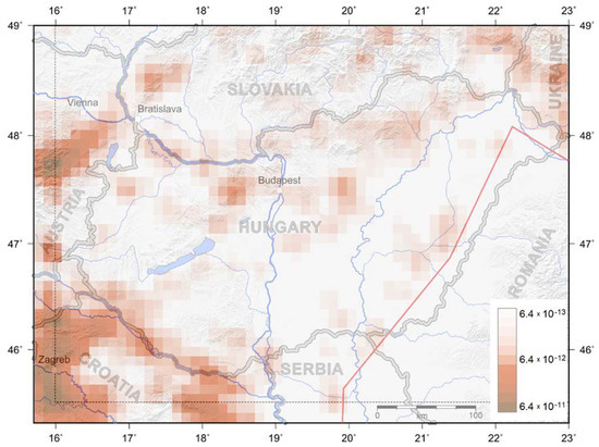
Figure 4.
Modelled background density plotted at 10 km pixel size (unit is .
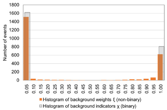
Figure 5.
Histogram of background weights over the epicenter catalogue of the study. A background weight close to 1 indicates a background event while a background weight close to zero indicates a triggered event.
4.2. Parameter Ranges
The estimation of parameter errors is not straightforward, since the errors obtained from analytical solutions can be different from simulation results [32]. Here, two simple tests to derive approximate error ranges are carried out: (1) In the first test, the MLE calculation is re-run on 20 simulated catalogues, using the preferred parameters for the simulation. Each simulated catalogue includes 2214 events, i.e., the same number as the actual study catalogue . For comparability with the actual catalogue, a fixed copy of the Petrinja mainshock is also included at the beginning of each simulation. Table 2 shows the minimum and maximum fitted parameters from these simulations. (2) In the second test, the sensitivity of the MLE calculation to a error in the magnitude of the Petrinja mainshock is reported.
Table 2.
Approximate error ranges for the estimated parameters and for the branching ratio .
4.3. Event Accumulation Test
The cumulative number of modelled events is obtained by integrating the conditional occurrence rate function [5]:
where the notation reflects the time-dependent area coverage of the study. Figure 6 shows the comparison of modelled and observed cumulative event numbers in the study period. The estimated number of non-observed Petrinja aftershocks is 155; this is the difference between the modelled and observed number of occurrences in the 1-day interval after the Petrinja mainshock. When the observed curve is corrected for this difference, the model captures the large Croatian earthquake sequences quite well. A weak point is the seemingly uneven observed background rate, which is not matched by the model: the underlying issue is that the southern part of the study area is unevenly covered by the patchwork of catalogues; this affects not only the southern extension margin but the southern edge of the core window too.
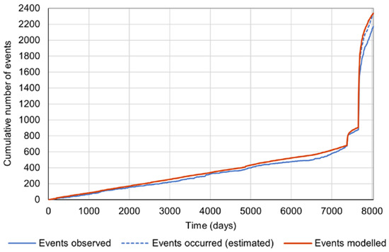
Figure 6.
Modelled versus observed event accumulation in the study period 2000–2021 for . The two large event surges late in the period correspond to the Zagreb and Petrinja, Croatia, 2020–2021 earthquake sequences. The model estimates that 155 occurrences in the Petrinja aftershock sequence are missing from the observed catalogue. Additionally, it is worth noting the step-up of the background rate from day 6576 (1 January 2018), which is the beginning of the period when the study area covers the extended window.
4.4. Poisson Goodness-of-Fit Test
The Poisson behaviour of the background process on the core area and of the full non-declustered process on the total modelled area is tested.
In the case of the background process, the modelled occurrence rate on the core area is at the magnitude threshold . When splitting the period into -day intervals, the event counts by interval should follow a Poisson distribution with a mean parameter according to the model. The outcome of chi-squared tests at a 0.95 confidence level is the following: at the magnitude threshold the catalogue typically fails the test for the period 2000–2021, but it passes the test for the period 2000–2010. At the magnitude threshold , with the Poisson mean scaled accordingly, the catalogue passes the test for the full 2000–2021 period. This can be explained by possible data deficiencies, i.e., missing small events along the periphery after the termination of Catalogue C in 2010.
In the case of the full non-declustered process, the time transformation , according to Equation (14), is used to convert the process into a stationary one [5]. When splitting the full period into -unit intervals of transformed time, the event counts by interval should follow a Poisson distribution with a mean parameter for . Chi-squared tests at a 0.95 confidence level fail the model at the threshold , but the model passes the tests at . This indicates that the observed process has some features at low magnitudes that this simplified model is unable to capture. Figure 7 shows some of the results of the Poisson goodness-of-fit tests.
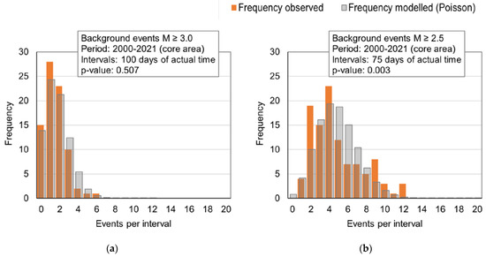
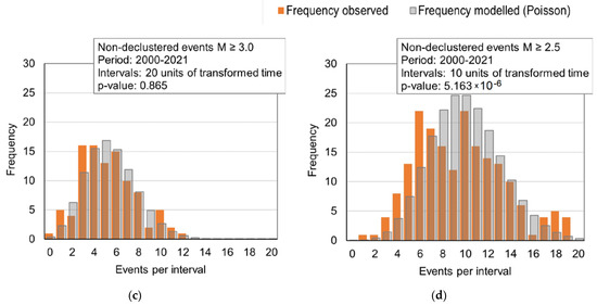
Figure 7.
Examples of chi-squared Poisson goodness-of-fit tests: The distribution of event counts per interval are compared to the modelled Poisson distribution for (a) background events in the core area, ; (b) background events in the core area, ; (c) all events, ; and (d) all events, .
The following three tests (i.e., distance test, time lag test, and triggering ability test) have been suggested and used with Japanese earthquake data by Zhuang et al. [8] in order to assess how well the space and time response functions of a model match the observations. The next subsections show the test results of this model with the Hungarian data.
4.5. Distance Test
This test compares the distribution of observed distances between trigger events and their aftershocks against the modelled space response function [8]. If an event is triggered by an event , the standardized distance between the two events can be defined as:
If the approximation of using a Gaussian space response function in the model is correct, then should follow a chi distribution with two degrees of freedom (or Rayleigh distribution with ). Since ancestor–descendant relationships between events cannot be identified unambiguously, the weights are introduced to express the fraction of event , which is triggered by event :
In order to build a histogram of the observed distribution of the sum of the values is taken in each standardized distance bin, where runs over and runs over .
The test results are shown in Figure 8, and they show a good fit. This outcome seems to be in contrast with the results of Zhuang et al., who conclude that the Gaussian space response form fits poorly to the Japan Meteorological Agency (JMA) catalogue data, as opposed to the power law, which shows good results. However, the authors used the Rayleigh distribution with the wrong parameter for the test, that is, instead of [8] (Equation (26), p. 7, Figure 7a, p. 10). With the correct theoretical distribution, the difference between the Gaussian model variant and the JMA data is much less than what the 2004 article suggests. In the case of this study, the additional spatial parameter also helps to achieve better results in this test.
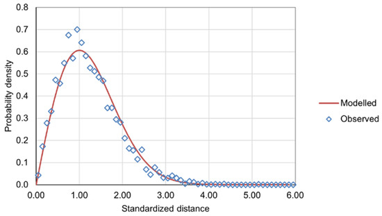
Figure 8.
Distance test results: reconstruction of the distribution of the standardized triggering distance from observations versus the modelled distribution.
4.6. Time Lag Test
The purpose of this test is to analyse the fit of the modelled time response function to the observations [8]. The test method is analogous to the distance test: instead of standardized distances, the distribution of the time lag between triggered events and their ancestors is reconstructed using the triggering weights , as defined in Equation (16). Unlike in the distance test, is allowed to run over the full catalogue rather than excluding the first day after the Petrinja mainshock; as a result, the incompleteness of the catalogue is also visible in the test outcome. Two views of the test output are shown in Figure 9: a plot of the probability density function (PDF) on a logarithmic scale and a complementary cumulative distribution function (CCDF) log–log plot, with the latter suggested as a more powerful diagnostic tool by Mignan [12].
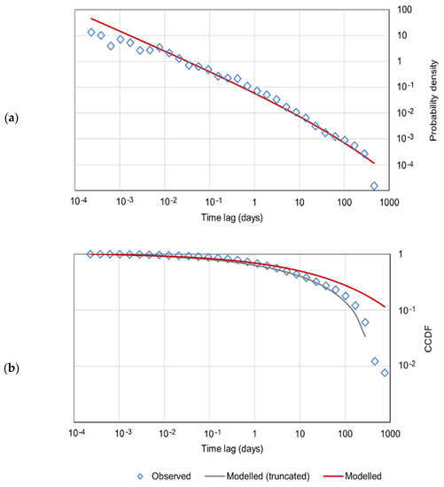
Figure 9.
Time lag test results: reconstruction of the distribution of the time lag between triggered events and their ancestors from observations. (a) Plot of probability density. (b) Plot of complementary cumulative distribution function (CCDF). To check the hypothesis that the deviation of the observed curve is explained by the time boundary effect, an alternative CCDF is also shown where the time lag is truncated at 400 days.
The test results show the following deviations: a downward deviation of the observed PDF from the model for very short time lags, apparently due to the incompleteness of early aftershock data in the Petrinja earthquake sequence. However, the test shows this deviation only at time intervals of less than days, that is, less than 15 min, whereas in the study catalogue, events with are missing from the initial part of the observed Petrinja aftershock sequence for more than days, that is, more than 2.4 h. The test also shows a downward deviation of the observed PDF from the model for very long time lags due to the boundary effect at the end of the study period. The latter effect also explains the downward deviation of the observed CCDF from the model.
4.7. Triggering Ability Test
This test compares the modelled and observed triggering ability of events by magnitude class [8]. The observed number of events triggered by an event is expressed as when using the triggering weights defined in Equation (16) while the modelled ultimate number is an exponential function of , and the expected number within the study period is obtained by restricting the integration bounds of the time responses. The test results are shown in Figure 10. While the test confirms the exponential trend, it also reveals an upward deviation from the model at low magnitudes. The graph suggests an exponential trend with a lower parameter than that of the model; the likely underlying effect is the anisotropy of aftershock clusters.
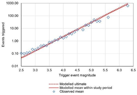
Figure 10.
Results of the triggering ability test: comparison of modelled and observed triggered event numbers by trigger event magnitude.
5. Parameter Downscaling Methods
5.1. Motivation for Downscaling
By downscaling, we mean the adaptation of the model parameters to smaller zones within the study area, where a stand-alone ETAS parameter estimation is not feasible due to insufficient data. Due to the data quality requirements of an ETAS study, the parameterization presented in the previous section relies on the instrumental catalogue data from the period 1996–2021, which are dominated by the 2020–2021 Croatian earthquake sequences. On the other hand, the largest historical occurrences within Hungary itself date to earlier than the study period. From the insurance industry point of view, a Hungarian earthquake model needs a regional parameterization, covering the central area around Budapest, since this area has the densest accumulation of insured property in the country. Furthermore, for a full coverage of the country, the geographical coverage gap along the Romanian border would need to be filled.
Section 5.2 and Section 5.3 describe an approach for adapting ETAS parameters to regional source zones, which incorporate historical earthquake data from a longer period. Therefore, we combined ETAS with standard techniques that have been used to parameterize stationary mainshock-only models. The zonation used in this study is based on the area sources of the SHARE project [26], with zone groupings for larger datasets. Figure 11 shows the map of the zones. The downscaling effort was restricted to the part of the zones within the core geographical window, defined between 45.5–49.0 N and 16.0–23.0 E.
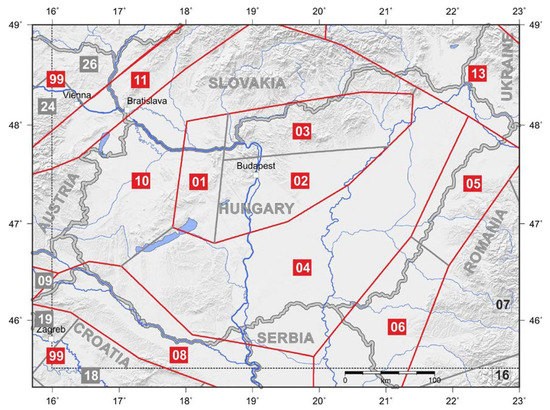
Figure 11.
Source zones and zone groupings used in the model, based on the area sources of the SHARE project [26]. The core geographical window is also displayed—the downscaled model covers the part of the zones falling within the core window. Zones 01–02–03, Zones 04–10, and Zones 05–06 are grouped for the model. The non-contiguous zones with grey labels are grouped for the model as the residual Zone 99. Zones with empty labels are not modelled.
5.2. Maximum Likelihood Estimation with Variable Observation Periods
In this section, we refer to the maximum likelihood estimation (MLE) method developed by Weichert [33]. In a nutshell, the aim of the estimation is to determine recurrence parameters for mainshocks, defined as the largest earthquakes in each cluster. The accumulation of mainshocks is assumed to follow a stationary Poisson point process with a constant recurrence rate . It is assumed that event magnitudes are independent and follow a truncated exponential distribution with decay parameter between the bounds and , according to Equation (4). Magnitudes are rounded and grouped into the magnitude bins . The length of the time interval when the historical event catalogue is complete varies by the magnitude class . The number of events in the respective magnitude class and completeness period is denoted by . The parameters , and are determined by prior expert judgement and are fixed in the estimation; the unknown parameters to be fitted are and . Under these assumptions, the event count is drawn from a Poisson distribution whose mean parameter is:
The calculus for finding the maximum of the corresponding likelihood function leads to the equations [33]:
The recurrence parameter estimates are obtained by solving Equation (18) for and then calculating from Equation (19). The strength of this MLE method is that it makes optimum use of available data by allowing magnitude-dependent observation periods. The method aims to find only temporal parameters. Its limitation is the reliance on a stationary Poisson event counting process, which normally restricts its application to declustered catalogues. Because the largest event in every cluster is selected, the estimated is expected to be lower than the parameter of the full population.
In our ETAS model context, the above MLE technique with variable observation periods could be straightforwardly adapted to find the parameters of the stationary Poisson background process while focusing on the initial event in each cluster rather than the largest one. For that, the calculation of the background weights and indicators according to Equations (10) and (11) would need to be extended to the full historical catalogue. Such an extension is possible, with the following caveats: due to incomplete data, the process may identify some triggered earthquakes as background events. In addition, the high epicenter uncertainty of historical events, and especially the use of macroseismic epicenters, may lead to implausible results, unless Equation (10) is adjusted to take this effect into account, e.g., by the convolution of the space distributions with error functions. However, we did not elaborate in this paper on this method and its results because this study took a different approach for the downscaling of ETAS parameters, as seen in Section 5.3.
5.3. Transformed Time Estimates
To be able to perform the MLE with variable observation periods on a non-declustered catalogue, the transformation was used, which converts the event counts into a stationary Poisson point process with unit rate [5], where is given by Equation (14).
When the event catalogue is incomplete, the part of the transformed time triggered by missing events is unknown. Given the ETAS parameters and the magnitude–frequency decay parameter , an estimate is provided for the transformed time interval length corresponding to the observation period where the observations are complete at magnitude threshold . Here, the space–time region is defined by a geographical zone and an observation period, and, as a simplification, it is assumed that the triggering effects crossing the boundaries of this region are negligible in both directions, which is a reasonable assumption if there are no major events close to the zone and period boundaries. This simplification allows for disregarding of the space–time integration bounds of the response functions and and ignoring all events outside the selected region. The total transformed time is divided into the following parts: (1) is the transformed time coming from the background process, (2) is the transformed time triggered by the above-threshold events, and (3) is the transformed time triggered by the below-threshold events. Given that the observed below-threshold events only set a lower bound, is unknown.
In Equation (22), is estimated by emulating iterations of the triggering process by tracing back every below-threshold event either to some above-threshold event or to the background:
where is the probability that the magnitude of an event is lower than according to Equation (24), and is the average reproduction rate of events below magnitude according to Equation (25). The truncation at is carried out to avoid double counting with .
Considering the lower bound in (22), the total estimated transformed time is then
The MLE framework with variable observation periods is used with the above time transformation for downscaling the ETAS parameters to zones. The starting values are the estimated overall parameters from Table 1. The background rate parameter is estimated for each zone from the 2000–2021 catalogue as , where is the length of this period in days; because the indicators are robust, they are not recalculated with the downscaled parameters. The time response shape parameters are left unchanged during the downscaling as most of the zone sub-catalogues have insufficient data to reparametrize them. The trigger scale parameter is rescaled to for each zone individually, and the parameter is adjusted by zone using the assumption. The transformed time intervals corresponding to the observation periods change with the rescaling. Starting from , the following iteration steps are repeated until convergence:
- Parameter is obtained by solving Equation (18) for the non-declustered event set in the transformed time, and is set equal to .
- The scaling factor is set such that for the non-declustered event set in the transformed time, where is calculated according to Equation (19).
There are no sufficient data by zone for an independent rescaling of the space response parameters and . Therefore, is kept unchanged while is rescaled to ; the latter assumption keeps the number of triggered events per unit of aftershock area approximately invariant.
6. Parameter Downscaling Results
6.1. Downscaled Parameters
The magnitude bounds are set at and , and the magnitude class width is . For simplicity, the same upper bound is used for all zones. Considering the maximum magnitudes of the model variants as in Tóth et al. [34], appears a conservative choice for the core geographical window. The largest homogenized magnitude in the historical catalogue observed within this area is which is estimated for the Érmellék 1834 earthquake. The observation periods by magnitude class are given in Table 3.
Table 3.
Observation periods by magnitude class.
The downscaled parameter estimates by zone are shown in Table 4. The obvious boundary effects at the Croatian edge of the core window make the transformed time estimates unreliable in Zone 99. For this zone all original parameters other than are kept unchanged. Because of data quality concerns, the parameters are not downscaled in the Romanian border Zone 05–06 either. As a placeholder solution for including the Romanian border area in the model, the kernel estimate of the background density and the declustering indicators are extended to Zone 05–06 without changing the original ETAS parameters while applying a 0.5 credibility weight to all events with questionable data quality (that is, all events in zone 05–06 whose only source is Catalogue C) and restricting the estimation of to the years 2000–2010. Another problem area is zone 13 on the northeastern periphery, where there is a very steep frequency decay at low-end magnitudes, which is a possible indication of the presence of an inhomogeneous sub-population. Therefore, in this zone, the lowermost magnitude classes—, for the estimation of , and , for transformed-time MLE—are excluded from the calculation. Thereby, some low-magnitude residual activity in this zone is left unmodelled.
Table 4.
Preferred ETAS parameters by zone after downscaling. The event numbers used for parameter downscaling and the implied branching ratios are also shown. The downscaling approaches were not applied to the Romanian border Zone 05–06 due to data deficiencies and to the residual Zone 99 due to boundary effects. Note that the background rates (without Zone 05–06) do not add up to the core area total in Table 1; the difference is due to the non-covered residual activity in Zone 13.
6.2. Sensitivity of the Downscaled Parameters
For assessing the robustness of the downscaling, the parameters are recalculated using two alternative parameterizations of the overall model from Section 4.2., i.e., with the two parameter sets calculated with alternative magnitudes of the Petrinja mainshock. The results of this calculation are shown in Table 5. Except for , the changes in most parameters are small. One cannot conclude from these results that the errors of the downscaled parameters are small; however, the test suggests that the sensitivity of these parameters to the overall parameterization is limited and that the parameters depend more strongly on the zone catalogues.
Table 5.
Alternative results for the downscaled parameters, starting from two alternative parameter sets of the overall model calculated with different magnitudes of the Petrinja mainshock, and , respectively (cf. Table 2).
6.3. Test of Long-Term Event Numbers by Zone
For this test, 500 stochastic catalogues were generated using the downscaled parameters and another 500 stochastic catalogues with the original parameters, each stochastic catalogue spanning 300 years. This provided a modelled distribution of event numbers by zone before and after downscaling, which were compared with the respective event numbers in the historical catalogue. The comparison focused on magnitudes , i.e., these events with a potential for insurance losses. Event numbers in the observation periods according to Table 3 were compared to these in the equivalent simulated periods by magnitude class. The test results are shown in Figure 12.
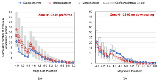
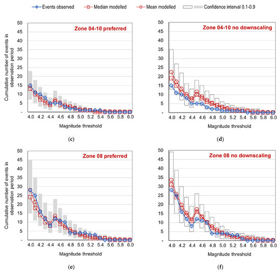
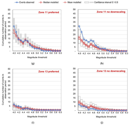
Figure 12.
Comparison of long-term event counts by zone, modelled and observed. The modelled distributions were obtained by generating 500 stochastic catalogues using the downscaled parameters and another 500 stochastic catalogues with the original parameters, each one spanning 300 years. The observation periods reflecting completeness differ by magnitude class; therefore, the event numbers shown are not always decreasing with the magnitude threshold. (a,c,e,g,i) Zone-by-zone downscaled model results. (b,d,f,h,j) Results for the same zones with parameters before downscaling, for comparison. (k,l) Results for Zones 05–06 and 99 where the downscaling approach is not used. (m,n) Results for the total modelled area, with and without downscaling.
6.4. Test of Event Accumulation by Zone, 2000–2021
The comparison of modelled versus observed cumulative event numbers (cf. Figure 6) is performed in this test for each zone separately. The results are shown in Figure 13. The model shows a better fit to the observations in the central Zones (01–02–03 and 04–10) than on the periphery; this can also reflect variations of underlying data quality. The biggest deviation is observed in Zone 13 where the smallest events were excluded from the downscaling to obtain a better fit to long-term event counts in higher magnitude classes.
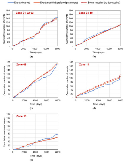
Figure 13.
Modelled versus observed event accumulation by zone in the study period 2000–2021 for . (a–e) Results of the test shown for each zone. Zones 05–06 and 99 with no downscaling are omitted.
7. Discussion and Conclusions
ETAS methodology has been applied to Hungarian earthquake data of the period 1996–2021. Despite the data challenges caused by moderate seismicity, we succeeded in fitting space–time ETAS parameters to recent instrumental data of the region, which include the 2020–2021 Croatian earthquake sequences. Our conclusions from the modelling exercise are the following:
- Poisson goodness-of-fit tests of the modelled versus the observed process show a satisfactory fit for events , which is appropriate for application in insurance. On the other hand, the same tests show significant deviations from the model at the magnitude threshold . These deviations at low magnitudes likely result from the inhomogeneities of the observed process between earthquake clusters, from data deficiencies, and possibly also from boundary effects at the edge of the modelled area or at the magnitude threshold.
- A stretched exponential time response function is used in the model. Based on the results of the event accumulation and time lag tests, we conclude that this time response form is appropriately fitted to the observed data. Deviations from the theoretical curve in the time lag test occur at very short time periods due to early aftershock incompleteness and at long time periods due to the time bounds of the observed catalogue. The modelled branching ratio implies a stable process. A systematic comparison of the stretched exponential function against the more commonly used modified Omori law as an alternative, however, was not part of this study.
- The model uses a Gaussian space response function with an allowance for epicenter error. The results of the standardized distance test show a good fit between the model and the observed data. The km value of the error parameter is consistent with the horizontal error estimates of the underlying catalogue. On the other hand, the fitted parameter possibly also absorbs a correction for a deviation of the data from the Gaussian space response model or from the constraint. An indication for this is that the 42-m value of the parameter is unlikely to reflect the aftershock radius of events by itself.
- After the overall ETAS parameter estimation, parameter adjustments for regional zones (downscaling) were also calculated. In this step, historical catalogue data going back to 1700 were incorporated. Despite the known limitations of the historical catalogue, we find it important that, in an insurance model for a moderately active region like Hungary, the most destructive historical events are taken into account for parameterization and for model testing. Even after the inclusion of historical events, the dataset used for downscaling is still dominated by recent instrumental data which have a lower magnitude threshold of completeness. The modelled event numbers were tested against long-term historical observations in the magnitude range relevant for insurance losses. For the total modelled area, the test outcomes show a good fit both with and without downscaling, with the modelled median numbers falling slightly closer to the observations with the non-downscaled parameters. However, downscaling provides clear improvements to the results by zone. While the parameters of the overall model are subject to significant uncertainties, the tests indicate that the downscaled parameters are only moderately sensitive to the variations of the overall parameters.
- For a Hungarian model, the central Zone 01–02–03 is especially important. In this zone, the downscaled model overestimates long-term event numbers in the 4.0–4.5 magnitude range. On the other hand, it gives better-fitting and more conservative results than the original parameterization for magnitudes , which is desirable in the case of a model for insurance applications. Zone 01–02–03 has experienced some notable event clusters in the 2000–2021 period, corresponding to the Oroszlány 2011, Tenk 2013, and Érsekvadkert-Iliny 2013–2015 events. The observed overall event accumulation in the zone is well-fitted to the downscaled model, as shown in Figure 13a; however, this graph masks the inhomogeneities between the two 2013 event sequences, which were geographically distant but overlapped in time.
Finally, we reflect on how the results of this study contribute to the planned application in insurance. In this study, only the first module of an earthquake risk model was covered, that is, a statistical model of event occurrences. With the help of this model, synthetic earthquake catalogues can be generated, representing sequences of events that may happen in the future and possibly cause losses. Unlike in those models where only mainshocks are modelled, the synthetic catalogues of this model also include aftershock sequences. However, the subset of the mainshocks can be extracted from the catalogues if a simplified model variant is preferred. If aftershocks are modelled, then the future scenarios are not independent from the past, as large earthquakes are followed by periods of increased seismic activity. This effect can be captured by the stochastic catalogue generator of this model if recent events are added to the simulation as fixed inputs, occurring before the simulated time interval.
The synthetic catalogues mentioned above will be used as a starting point for simulating insurance losses when the full model is in place. Future work on the model will focus on developing those modules that were not discussed in this study: the ground motion attenuation and the vulnerability modules. Another possible area of future work is to extend the geographical coverage of the model to other Central European countries.
Author Contributions
Conceptualization, J.C.-B. and P.S.; Methodology, P.S.; Software, P.S.; Formal analysis, P.S.; Data curation, L.T.; Writing—original draft preparation, P.S.; Writing—review and editing, J.C.-B. and L.T.; Supervision, J.C.-B. and L.T.; Project administration, J.C.-B. All authors have read and agreed to the published version of the manuscript.
Funding
This research was fully funded by the UNIQA Insurance Group AG.
Data Availability Statement
Original datasets analysed in this study are mostly publicly available and can be found here: http://mek.niif.hu/04800/04801/ (accessed on 5 February 2023), http://www.isc.ac.uk/iscbulletin/search/ (accessed on 5 February 2023), https://earthquake.usgs.gov/earthquakes/search/ (accessed on 5 February 2023), http://www.georisk.hu/Bulletin/bulletinh.html (accessed on 5 February 2023), http://www.georisk.hu/Tajekoztato/tajekoztato.html (accessed on 5 February 2023). Other, pre-processed data presented in this study are available on request from the author: László Tóth; email: toth@georisk.hu.
Acknowledgments
The authors acknowledge the financial support of the UNIQA Insurance Group AG, Wien, Austria and especially Kurt Svoboda and Roman Schneider. The authors also thank Balázs Sághy at UNIQA Biztosító Zrt., Budapest, Hungary for all his support and encouragement given to this research, and for his help with software tools.
Conflicts of Interest
The authors declare no conflict of interest.
References
- Directive 2009/138/EC of the European Parliament and of the Council of 25 November 2009 on the Taking-Up and Pursuit of the Business of Insurance and Reinsurance (Solvency II). Available online: https://eur-lex.europa.eu/eli/dir/2009/138/oj (accessed on 5 February 2023).
- Commission Delegated Regulation (EU) 2015/35 of 10 October 2014 Supplementing Directive 2009/138/EC of the European Parliament and of the Council on the Taking-Up and Pursuit of the Business of Insurance and Reinsurance (Solvency II). Available online: https://eur-lex.europa.eu/eli/reg_del/2015/35/oj (accessed on 5 February 2023).
- Petrinjski Potresi: Prosinac 2020.—Prosinac 2021.—Geofizički Odsjek. Godina Dana od Razornog Potresa Kod Petrinje. Available online: https://www.pmf.unizg.hr/geof/seizmoloska_sluzba/potresi_kod_petrinje/2020–2021 (accessed on 16 December 2022).
- Oros, E.; Placinta, A.O.; Popa, M.; Diaconescu, M. The 1991 Seismic Crisis in the West of Romania and Its Impact on Seismic Risk and Hazard Assessment. Environ. Eng. Manag. J. 2019, 19, 609–623. [Google Scholar] [CrossRef]
- Ogata, Y. Statistical models for earthquake occurrences and residual analysis for point processes. J. Am. Stat. Assoc. 1988, 83, 9–27. [Google Scholar] [CrossRef]
- Ogata, Y. Space-Time Point-Process Models for Earthquake Occurrences. Ann. Inst. Stat. Math. 1998, 50, 379–402. [Google Scholar] [CrossRef]
- Zhuang, J.; Ogata, Y.; Vere-Jones, D. Stochastic Declustering of Space-Time Earthquake Occurrences. J. Am. Stat. Assoc. 2002, 97, 369–380. [Google Scholar] [CrossRef]
- Zhuang, J.; Ogata, Y.; Vere-Jones, D. Analyzing earthquake clustering features by using stochastic reconstruction. J. Geophys. Res. 2004, 109, B05301. [Google Scholar] [CrossRef]
- Hardebeck, J. Appendix S–Constraining Epidemic Type Aftershock Sequence (ETAS) Parameters from the Uniform California Earthquake Rupture Forecast, Version 3 Catalog and Validating the ETAS Model for Magnitude 6.5 or Greater Earthquakes. In Uniform California Earthquake Rupture Forecast, Version 3 (UCERF3)—The Time-Independent Model, Field, E.H., Biasi, G.P., Bird, P., Dawson, T.E., Felzer, K.R., Jackson, D.D., Johnson, K.M., Jordan, T.H., Madden, C., Michael, A.J., et al., U.S. Geological Survey Open-File Report 2013–1165, 97 p., California Geological Survey Special Report 228, and Southern California Earthquake Center Publication 1792. Available online: https://pubs.usgs.gov/of/2013/1165/ (accessed on 5 February 2023).
- Veen, A.; Schoenberg, F.P. Estimation of Space–Time Branching Process Models in Seismology Using an EM–Type Algorithm. J. Am. Stat. Assoc. 2008, 103, 614–624. [Google Scholar] [CrossRef]
- Ogata, Y.; Zhuang, J. Space–time ETAS models and an improved extension. Tectonophysics 2006, 413, 13–23. [Google Scholar] [CrossRef]
- Mignan, A. Modeling aftershocks as a stretched exponential relaxation. Geophys. Res. Lett. 2015, 42, 9726–9732. [Google Scholar] [CrossRef]
- Stallone, A.; Marzocchi, W. Empirical evaluation of the magnitude-independence assumption. Geophys. J. Int. 2019, 216, 820–839. [Google Scholar] [CrossRef]
- Turcotte, D.L.; Holliday, J.R.; Rundle, J.B. BASS, an alternative to ETAS. Geophys. Res. Lett. 2007, 34, L12303. [Google Scholar] [CrossRef]
- Zhuang, J.; Werner, M.J.; Harte, D.S. Stability of earthquake clustering models: Criticality and branching ratios. Phys. Rev. E 2013, 88, 062109. [Google Scholar] [CrossRef]
- Guo, Y.; Zhuang, J.; Zhou, S. A hypocentral version of the space–time ETAS model. Geophys. J. Int. 2015, 203, 366–372. [Google Scholar] [CrossRef]
- Guo, Y.; Zhuang, J.; Zhou, S. An improved space-time ETAS model for inverting the rupture geometry from seismicity triggering. J. Geophys. Res. Solid Earth 2015, 120, 3309–3323. [Google Scholar] [CrossRef]
- Seif, S.; Mignan, A.; Zechar, J.D.; Werner, M.J.; Wiemer, S. Estimating ETAS: The effects of truncation, missing data, and model assumptions. J. Geophys. Res. Solid Earth 2016, 122, 449–469. [Google Scholar] [CrossRef]
- Magyarországi Földrengések Évkönyve. Hungarian Earthquake Bulletin 1995–2019; GeoRisk: Budapest, Hungary, 1996–2020; HU ISSN 1219-963X; Available online: http://www.georisk.hu/Bulletin/bulletinh.html (accessed on 5 February 2023).
- MABISZ: A Decemberi Földrengések Magyar Kárbejelentéseinek a Száma Meghaladja a Horvátországit. Available online: https://mabisz.hu/a-decemberi-foldrengesek-magyar-karbejelenteseinek-a-szama-meghaladja-a-horvatorszagit/ (accessed on 16 December 2022).
- Zsíros, T. A Kárpát-Medence Szeizmicitása és Földrengés Veszélyessége: Magyar Földrengés Katalógus (456–1995), MTA GGKI: Budapest, Hungary, 2000. Available online: https://mek.oszk.hu/04800/04801/ (accessed on 5 February 2023).
- International Seismological Centre. On-Line Bulletin. 2022. Available online: https://doi.org/10.31905/D808B830 (accessed on 29 April 2021).
- U.S. Geological Survey. Available online: https://earthquake.usgs.gov/earthquakes/search/ (accessed on 29 April 2021).
- Grünthal, G.; Wahlström, R.; Stromeyer, D. The unified catalogue of earthquakes in central, northern, and northwestern Europe (CENEC)—Updated and expanded to the last millennium. J. Seism. 2009, 13, 517–541. [Google Scholar] [CrossRef]
- GeoRisk—Földrengés Mérnöki Iroda—Earthquake Engineering. Havi Földrengés Tájékoztató (Monthly EQ list). Available online: http://www.georisk.hu/Tajekoztato/tajekoztato.html (accessed on 5 February 2023).
- Woessner, J.; Laurentiu, D.; Giardini, D.; Crowley, H.; Cotton, F.; Grünthal, G.; Valensise, G.; Arvidsson, R.; Basili, R.; Demircioglu, M.B.; et al. The 2013 European Seismic Hazard Model: Key components and results. Bull. Earthq. Eng. 2015, 13, 3553–3596. [Google Scholar] [CrossRef]
- Utsu, T. Aftershock and earthquake statistics (I): Some parameters which characterize an aftershock sequence and their interrelations. J. Fac. Sci. Hokkaido Univ. 1969, 3, 129–195. [Google Scholar]
- Hainzl, S.; Christophersen, A.; Enescu, B. Impact of Earthquake Rupture Extensions on Parameter Estimations of Point-Process Models. Bull. Seism. Soc. Am. 2008, 98, 2066–2072. [Google Scholar] [CrossRef]
- Felzer, K.R.; Becker, T.W.; Abercrombie, R.E.; Ekström, G.; Rice, J.R. Triggering of the 1999MW7.1 Hector Mine earthquake by aftershocks of the 1992MW7.3 Landers earthquake. J. Geophys. Res. Atmos. 2002, 107, ESE 6-1–ESE 6-13. [Google Scholar] [CrossRef]
- Fletcher, R.; Powell, M.J.D. A Rapidly Convergent Descent Method for Minimization. Comput. J. 1963, 6, 163–168. [Google Scholar] [CrossRef]
- Burkhard, M.; Grünthal, G. Seismic source zone characterization for the seismic hazard assessment project PEGASOS by the Expert Group 2 (EG1b). Swiss J. Geosci. 2009, 102, 149–188. [Google Scholar] [CrossRef]
- Wang, Q.; Schoenberg, F.P.; Jackson, D.D. Standard Errors of Parameter Estimates in the ETAS Model. Bull. Seism. Soc. Am. 2010, 100, 1989–2001. [Google Scholar] [CrossRef]
- Weichert, D.H. Estimation of the earthquake recurrence parameters for unequal observation periods for different magnitudes. Bull. Seism. Soc. Am. 1980, 70, 1337–1346. [Google Scholar] [CrossRef]
- Tóth, L.; Győri, E.; Mónus, P.; Zsíros, T. Seismic Hazard in the Pannonian Region. In The Adria Microplate: GPS Geodesy, Tectonics and Hazards; Pinter, N., Ed.; Springer: Dordrecht, The Netherlands, 2006; pp. 369–384. [Google Scholar] [CrossRef]


Disclaimer/Publisher’s Note: The statements, opinions and data contained in all publications are solely those of the individual author(s) and contributor(s) and not of MDPI and/or the editor(s). MDPI and/or the editor(s) disclaim responsibility for any injury to people or property resulting from any ideas, methods, instructions or products referred to in the content. |
© 2023 by the authors. Licensee MDPI, Basel, Switzerland. This article is an open access article distributed under the terms and conditions of the Creative Commons Attribution (CC BY) license (https://creativecommons.org/licenses/by/4.0/).