Abstract
THz-Time domain spectroscopic imaging is demonstrated combining a robotic scanning method with continuous signal acquisition and holographic reconstruction of the object to improve the imaging resolution. We apply the method to a metallic Siemens star in order to quantify resolution and to wood samples to demonstrate the technique on a non-metallic object with an unknown structure.
1. Introduction
The THz spectral range covering frequencies between 0.1 THz and 10 THz or, alternatively, wavelengths between 0.03 mm and 3 mm is used for sensing applications in non-destructive evaluation, material characterisation, medical and chemical analyses, and security and communication [1]. THz material properties, such as absorption and thus penetration depth, all depend on the THz wavelength. To obtain a map of THz properties, THz imaging has been developed over the past two decades [2,3]. THz imaging using a single wavelength source is evolving towards real-time applications [4,5]. To obtain a map of spectral information, THz spectral imaging techniques have been developed and were reviewed recently [6]. Spectral imaging can be performed using a tunable THz source, but here we focus on THz-Time Domain Spectroscopy (TDS) for obtaining spectral information with a single point detector [7]. Due to the short THz pulses, they are often used in time-of-flight measurements to determine layered structures, e.g., in the inspection of cultural heritage [8,9], while spectral imaging has found applications in the assessment of, e.g., agricultural products [10]. It is based on scanning the beam using mirrors [11,12] or on scanning the object. For measurements in transmission, scanning the object is favorable, typically using an x–y translation stage [13,14]. However, such stages might not be ideal, as their travel range and sample mounting possibilities are restricted once a handling system is devised. In contrast, the six axes of a robot arm offer more flexibility, both in travel range and sample handling. Robot-assisted imaging is being developed in medical applications [15] as well as non-destructive evaluation [16] and is being explored in THz applications [17,18,19].
The lateral resolution of THz imaging is typically dependent on the beam size of the THz source on the object. To improve the lateral resolution, aperture-based near-field imaging has been reported [7]. However, reducing the aperture diameter to improve lateral resolution reduces the radiation level on the detector, causing a trade-off between resolution and signal-to-noise ratio. In addition, near-field imaging using apertures is impractical for larger objects, as the object would need to be scanned in close vicinity of the aperture or would need to be lifted off and be approached again for each measurement, which renders the procedure time-consuming. On the other hand, increasing the distance of the object surface from the aperture would jeopardize resolution, as the (sub-wavelength) aperture diffracts the beam to a larger spot. In holographic THz imaging, the lateral resolution is limited by the acceptance angle of the detector array, which is related to the ratio of detector size to object distance [20]. The phase delay from the measurement point can be retrieved in TDS from the Fourier spectrum [21]. A THz-TDS image thus contains both the amplitude and phase of the signal, so that a holographic reconstruction [5] to the object plane can be performed.
In this paper, we present THz-TDS imaging combining a robotic scanning method with continuous signal acquisition and holographic reconstruction of the object to improve the resolution. We apply the method to a metallic Siemens star in order to quantify resolution and to wood samples with birefringent optical properties [22] to demonstrate the technique on a structured non-metallic object.
2. Materials and Methods
2.1. TDS Experimental Setup
A commercial THz-TDS system TeraFlash (TOPTICA Photonics AG, Graefelfing, Germany) with a bandwidth from 0.2 THz to 6.0 THz was used. The beam from the emitter was focused onto the sample using two off-axis parabolic mirrors shown in Figure 1 (artistic illustration). For some experiments, a metallic aperture with a diameter of was placed in the focused beam to restrict the spot size. Two polarizers P1 and P2 (wire grid polarizers G30X10-S from SEMIC RF, Taufkirchen, Germany) allowed setting the polarisation direction before the sample and to analyse the polarisation after the sample, respectively. Raw spectra of the TDS were collected with an in-house extension of the TeraFlash control program written in LabVIEW. The samples were mounted on a robot arm and scanned line by line in a meander-like manner with constant speed (2 mm/s to 5 mm/s) at a specific distance (0.1 mm to 5 mm) from the aperture mask.
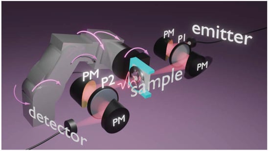
Figure 1.
Schematic representation of the THz-TDS setup for measurements using a robot arm for sample scanning (PM: off-axis parabolic mirror, P1, P2: polarizer).
2.2. Robotics
In order to allow for 2D scans of the sample, a precise six-axis industrial robot arm (Meca500, Mecademic Robotics, Montreal, QC, Canada) with a positioning repeatability of was used. An electric parallel finger gripper (MEGP-25E, Mecademic Robotics, Canada) was used to control the sample position in the THz beam using a custom-written Python program. Custom gripper fingers were 3D-printed (Material: PolyTerraTM PLA, Polymaker Inc., Shanghai, China; Printer: Prusa i3 MK3S+, Prusa Resarch S.R.O., Prague, Czech Republic) and used to clamp the PTFE-based sample holder with the robot’s end effector. The approach of the sample to the aperture mask was conducted with a manual controlled robot operation in a rectangular coordinate system and visually supervised by the robot operator. Subsequently, the sample was moved horizontally across the mask aperture with a constant velocity. At the end of each line, the position of the robot end effector was recorded along with a timestamp in order to be synchronized with the recorded THz spectra.
2.3. Synchronization
The LabVIEW-based THz-TDS control program stored spectra at a varying rate from 9 spectra per second to 16 spectra per second in an unsynchronized manner. The THz-TDS controller hardware did not allow direct access to the internal timestamps. Consequently, every spectrum was tagged with a software (LabVIEW) based timestamp, which is derived from the computer’s CPU clock and can be assumed to be highly correlated with the effective measuring time. The Python control program of the robot ran on the same computer as the THz-TDS control software and used timestamps derived from the same CPU clock. Due to the hardware abstraction layers and implementation details of the LabVIEW and Python frameworks, offsets may have occurred due to drifting and latencies, which are varying over time. In practice, it was hard to quantify the resulting time scales. A generous, educated guess for the upper error bound is 40 ms, which for the scanning speeds used in this paper results in an error smaller than the expected experimental resolution limit. This allowed the usage of the two timestamps for the synchronization of each measured THz-TDS spectrum with a sample position. However, we still had to consider a small, constant offset originating from the measurement procedure itself, which was determined for a specific scanning speed setting from two consecutive scan lines of the resolution target. Figure 2 shows a typical mapping of the scan positions of the spectra with the robot movement.
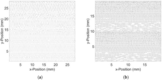
Figure 2.
Synchronization using timestamps of TDS and robot: (a) a scan speed of 5 / and a total scanning time of 6 ; (b) a scan speed of 2 / and a total scanning time of 20 .
For data collection times above around 7 min, short sequences of spectra are missing and impair reliable data collection. As a solution, the scan was split into several parts, storing the data to disk in chunks. This is illustrated in Figure 2, where the spectra were collected in two parts, with scanning times of 10 min each. Image data were calculated using a regular grid with a pixel distance of half of the line spacing and attributing the spectrum of the scan position with the shortest Euclidean distance. A Gaussian kernel with a width of 1 pixel was then applied to the image for smoothing.
2.4. Samples
2.4.1. Resolution Target
As a resolution target, a nine-spoke Siemens star with a diameter of 12 was fabricated from a thick metal sheet using laser ablation. It was attached to a 29 mm × 33 mm × 2.2 mm PTFE holder using tape above and below the star.
2.4.2. Wood Samples
Wood sample #1 (33 mm × 33 mm × 2 mm) is an LR cut from a spruce trunk, showing annual rings of different widths where L is the longitudinal and R is the radial direction. For localization purposes. a 1 mm hole was drilled into the lower left corner of the sample.
Wood sample #2 is a 2.65 mm thick RT cut of a spruce branch where R is the radial and T is the tangential direction. It shows concentric annual rings and a dark core of about 3 mm. Samples are shown in Figure 3. For both wood samples. the inner part was measured by attaching them to a 33 mm × 33 mm × 2 mm square PTFE holder with a 16 mm × 16 mm × 2 mm opening using double-sided tape.
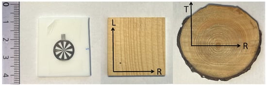
Figure 3.
Resolution sample (left), wood sample #1; LR spruce (middle), wood sample #2; RT spruce from branch (right), scale in cm; wood directions R, T, and L are shown in the figure.
2.5. Simulation of TDS Experiment
The TDS experiment was simulated using holographic reconstruction. The reconstruction method was based on evaluating the Rayleigh–Sommerfeld diffraction integral by use of the fast Fourier transform. The forward propagation of a complex wave field with wavelength from a plane at , , to a plane at , is obtained by [23,24].
where is the two-dimensional Fourier spectrum, and are the Fourier frequencies for at . Back propagation from a given diffraction field to a source field can be obtained by the complex conjugate in Equation (1).
The simulation of the TDS experiment was conducted by propagating the THz field in steps from the source to the detector as illustrated in Figure 4.
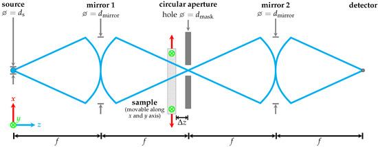
Figure 4.
Simulation scheme of TDS experiments (not to scale).
Starting with a point source or a source with a Gaussian intensity distribution of width , the field is propagated to a parabolic mirror of diameter at distance f corresponding to the focal length of the mirror. The ratio of defines the numerical aperture. The field is then mirrored (by taking the complex conjugate of the field) and propagated by to the sample position. The field is then modified by the transmission function of the sample at position x and y and propagated by to the focal point of the experiment. Here, a metal mask with an aperture of diameter is applied to the field. The field is then propagated by f to a parabolic mirror. The field is mirrored again and propagated to the detector, where the complex intensity is integrated. Parameters of the simulations are the sample position in x and y, the wavelength , , and .
3. Results
3.1. Resolution Target
In a first experiment, the resolution target was scanned without using a mask. The intensity images and their simulation are shown in Figure 5 top and bottom row, respectively. The resolution is strongly frequency-dependent, as expected for the wavelength limited resolution d of such an optical setup given by
where is the numerical aperture and the wavelength. If we assume for our setup , the resolution limits are estimated to d = 2 mm for 0.5 THz and d = 0.5 mm for 2.0 THz.
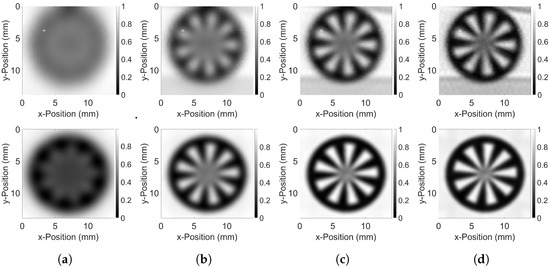
Figure 5.
Resolution target images without mask for selected frequencies. Measurement (top) and simulation (bottom); (a) 0.5 THz; (b) 1.0 THz; (c) 1.5 THz; (d) 2.0 THz.
Next, we looked at a configuration where the sample was positioned very close ( = 0.5 mm) to an aperture of diameter . Figure 6 shows the measured images in the top row and the simulated images in the bottom row. The resolution is much improved compared to Figure 5 and only slightly frequency-dependent. At low frequency, especially at 0.5 THz, the centre of the Siemens star shows interference effects, which can be attributed to the finite distance from the mask. This effect can be seen in both the measurement and the simulations.
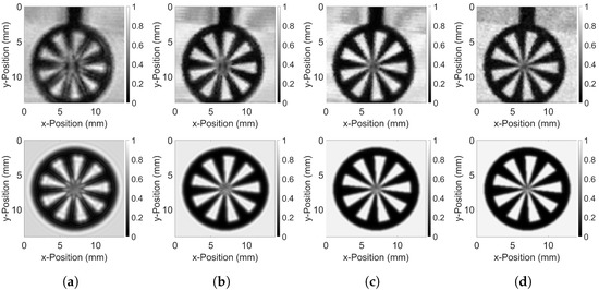
Figure 6.
Resolution target images for selected frequencies taken with a 0.5 mm mask at a distance of 0.5 mm. Measurement (top row) and simulation (bottom row): (a) 0.5 THz; (b) 1.0 THz; (c) 1.5 THz; (d) 2.0 THz.
3.2. Holographic Reconstruction
In a third configuration, the sample was put at a distance of 5 from the mask. The images in the first two rows in Figure 7 show the typical intensity pattern of a hologram expected from such a resolution target.
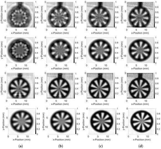
Figure 7.
Resolution target images at distance mm from mask: measurement: (first row), and simulations (second row); holographic reconstruction of measurements (third row) and holographic reconstruction of simulations (fourth row); (a) 0.5 THz; (b) 1.0 THz; (c) 1.5 THz; (d) 2.0 THz.
Measurements and simulations are again in good agreement. Back propagation of the complex images taken at 5 to the sample position at 0 yields a good reconstruction of the original target, as shown in the third and fourth row in Figure 7. For the simulation, we assumed a spot size of 0.5 mm instead of a point source to better match the measured images.
3.3. Birefringence in Wood
An LR cut of a spruce sample (wood sample #1) was used because this cut is known to be birefringent [22] and at the same time shows the annual ring structure. The principal axes of birefringence can be assumed parallel and perpendicular to the annual rings. The sample was scanned two times, once with the annual rings perpendicular () to the polarization and once with the annual rings parallel () to the polarization. The intensity and phase images for selected frequencies are shown in Figure 8.
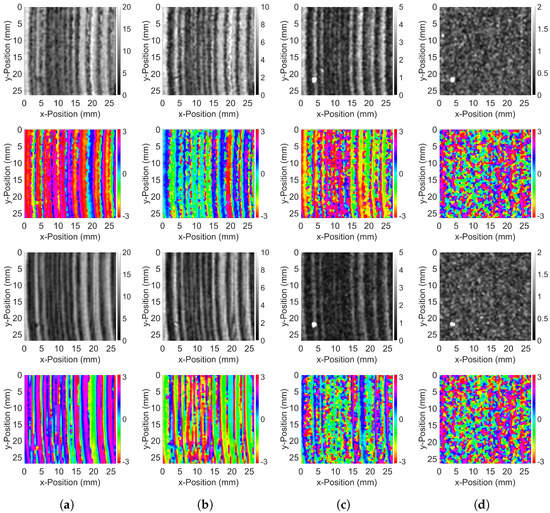
Figure 8.
Intensity (gray scale) and phase images (color scale) of the wood sample #1. Sample orientation of annual rings with respect to polarization: (top two rows) and (bottom two rows): (a) 0.5 THz; (b) 1.0 THz; (c) 1.5 THz; (d) 2.0 THz.
The samples show strong anisotropic properties. For a given frequency, the phase images for the two orientations show an overall phase shift, a known consequence of birefringence. Furthermore, the images with generally show a lower transmission, resulting in darker images as compared to the images with . This is in line with the direction-dependent conductivity in the microfibrils in wood, which are preferably oriented along the longitudinal direction L.
For the RT cut, wood sample #2, the principal axes of birefringence are expected to be position-dependent. In order to assess the full local anisotropic optical properties, the sample was imaged in four sets of polarizer orientations: [, ] = [, ], [, ], [, ], and [, ]. This allowed the local determination of all four complex Jones matrix elements. Figure 9 shows intensity and phase images for all four polarizer orientations for 0.5 THz.
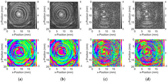
Figure 9.
Intensity (top row) and phase images (bottom row) at 0.5 THz for wood sample #2 for measurements at different polarizer orientations [, ]: (a) [, ]; (b) [, ]; (c) [, ]; (d) [, ].
In general, the influence of the annual ring structure is clearly visible. The intensity and phase images pairs for the bright field configurations ([, ], [, ]) and the dark field configurations ([, ], [, ]) are very similar indicating the absence of optical activity. The dark diagonal lines in the dark field configurations are isoclinics. A birefringence with principal axes parallel and perpendicular to the polarizers will block the field completely, which is not the case for other directions.
4. Discussion
With the above results, we present a versatile technique for THz spectral imaging. In the following, we will discuss several aspects in view of future use. Two scanning methods were used, either scanning the sample very close to the aperture or scanning at a distance and using holographic reconstruction.
The use of a small aperture close to the sample was key to a decent resolution, including the longer wavelengths. It allows us to overcome the resolution limit given by the wavelength and the small numerical aperture of the setup. Apart from the wavelength, the limiting factors for resolution are mask aperture, sample distance, and sample thickness. Estimated resolutions extracted from the images in Figure 5, Figure 6 and Figure 7 are summarized in Table 1. They illustrate that, using an aperture mask, the resolution is not governed by the limit given by Equation (3) but rather by the size of the aperture mask.

Table 1.
Resolutions for selected frequencies compared to resolution limit.
The presented simulation of the imaging method is in good agreement with the measurements. It can be used to optimize the setup for a specific imaging task.
The annual ring structure of wood samples is imaged nicely, and the polarisation-dependent images are consistent with a structured birefringent material. The increasing absorption of THz radiation with frequency puts an upper limit of about 2 THz for imaging wood structures. A local mapping of refractive indices and extinction coefficients is not straightforward due to diffraction and interference effects within a sample of a thickness exceeding the wavelength. Here, modelling using multilayer field propagation could give more insights.
The use of holographic reconstruction has the potential for imaging structures embedded in a homogenous matrix or a micro-fluidic device. Furthermore, it allows reconstruction to curved sample surfaces from a planar scan. In order to increase the accuracy of the reconstruction, the illuminated region of the sample could be increased. However, this might negatively impact the intensity passed through the aperture. One may argue that the scanning of a sample close to a mask does not correspond to a holographic data collection. This would only be the case if the sample were illuminated by an infinite plane wave. In this case, scanning a sample before a fixed mask would be equivalent to scanning a mask (representing a pixel of a camera) before a fixed sample. However, the reconstruction works well for a focusing illumination of limited spot size. If holographic reconstruction is used, the spot size on the sample can be optimized in order to allow for proper reconstruction, but still maintaining enough intensity hitting the aperture. A spot size in the order of seems reasonable.
The use of the robot is a new approach compared to traditional XY stages, where only the sample can be scanned. It offers a more flexible way to position the sample. It allows changing the distance to the aperture mask, and the sample can be put in different orientations with respect to the polarization of the incident light. Polarization-dependent measurements can be realized in three ways: (1) by rotating the sample by the robot, (2) dropping and re-picking the sample rotated by 90 (used for wood sample #1), and (3) by setting the polarizer angles manually to (used for wood sample #2). With the robot arm, it is possible to scan a non-planar convex object of known surface shape by minimizing the distance of the sample to the aperture mask and choosing the orientation of the sample with respect to the incident beam. Furthermore, repeatable measurement, e.g., accounting for changing humidity conditions are possible.
The higher jitter in the annual ring structure in the images for in Figure 8 indicates that the synchronization of spectrum collection is not perfect and demonstrates one limitation of our scanning setup. This may have led to a slightly lower resolution in the horizontal scanning direction compared to the vertical direction. The extraction of spectra from the available time domain spectrometer control software has its limitation with respect to achievable data rate as well as proper synchronization. However, for the images collected for this work, its influence on resolution is small compared to other factors.
Today’s state-of-the-art TDS systems may offer much faster spectrum collection including in time data storage. Here, it is even more important that the control software allows for low level hardware access or at least hardware clock/timestamp synchronization. In addition, the saving of spectra has to be optimized for reliability at high data rates with low latency.
The rather long scanning times of 6 min to 20 min for our images are due to our specific TDS system and its limited access to the raw spectra. We see a high potential for shorter sample scanning times. With a newer system a speed up to a factor of five seems reasonable, provided that fast data storage is available. Spectrum collection of current TDS systems can exceed 50 spectra per second. Furthermore, an optimization of scanning speed, sample scan area, and aperture size in view of the targeted resolution allows an optimization of scanning times.
5. Conclusions
The THz-TDS imaging method combining a robotic scanning method with continuous signal acquisition has high potential for THz spectral imaging. In particular, the possibility of holographic reconstruction opens new ways to access structures from a distance. Key factors for good resolution are a small aperture mask, fast collection of THz spectra, the ability to move and position the sample very accurately, and to correctly synchronize spectral data with sample positions. A THz source with a higher power as well as a more sensitive detector would allow for using even smaller apertures. The use of robots allows for flexible scanning options and reliable, repetitive imaging tasks. This method can find applications to non-destructive testing from medical to industrial applications that currently use THz imaging.
Author Contributions
D.B. and R.B. designed and guided the robot integration; L.N.C. and S.L.G. realised the robot scanning and performed the measurements; E.H. contributed to the holographic reconstruction method; E.M. contributed to the TDS setup and its visualization; D.S. designed, implemented, and tested the TDS data collection software; P.Z. led the project, was responsible for data evaluation and simulations and drafted the manuscript. All authors have read and agreed to the published version of the manuscript.
Funding
This research was funded by the Swiss National Science Foundation, grant number 200021-179061/1.
Institutional Review Board Statement
Not applicable.
Informed Consent Statement
Not applicable.
Data Availability Statement
Data underlying the results may be obtained from the authors upon reasonable request.
Acknowledgments
The authors would like to thank Markus Rüggeberg and Jingming Cao for providing and preparing the wood samples.
Conflicts of Interest
The authors declare no conflict of interest.
Abbreviations
The following abbreviations are used in this manuscript:
| THz | Terahertz |
| TDS | Time domain spectroscopy |
| NA | Numerical Aperture |
References
- Dhillon, S.S.; Vitiello, M.S.; Linfield, E.H.; Davies, A.G.; Hoffmann, M.C.; Booske, J.; Paoloni, C.; Gensch, M.; Weightman, P.; Williams, G.P.; et al. The 2017 terahertz science and technology roadmap. J. Phys. D Appl. Phys. 2017, 50, 043001. [Google Scholar] [CrossRef]
- Mittleman, D.M. Twenty years of terahertz imaging. Opt. Express 2018, 26, 9417–9431. [Google Scholar] [CrossRef] [PubMed]
- Hu, B.; Nuss, M. Imaging with terahertz waves. Opt. Lett. 1995, 20, 1716–1718. [Google Scholar] [CrossRef] [PubMed]
- Guerboukha, H.; Nallappan, K.; Skorobogatiy, M. Toward real-time terahertz imaging. Adv. Opt. Photonics 2018, 10, 843–938. [Google Scholar] [CrossRef]
- Valzania, L.; Zhao, Y.; Rong, L.; Wang, D.; Georges, M.; Hack, E.; Zolliker, P. THz Coherent Lensless Imaging. Appl. Opt. 2019, 58, G256–G275. [Google Scholar] [CrossRef] [PubMed]
- Bandyopadhyay, A.; Sengupta, A. A Review of the Concept, Applications and Implementation Issues of Terahertz Spectral Imaging Technique. IETE Tech. Rev. 2022, 39, 471–489. [Google Scholar] [CrossRef]
- Wang, Q.; Xie, L.; Ying, Y. Overview of imaging methods based on terahertz time-domain spectroscopy. Appl. Spectrosc. Rev. 2022, 57, 249–264. [Google Scholar] [CrossRef]
- Picollo, M.; Fukunaga, K.; Labaune, J. Obtaining noninvasive stratigraphic details of panel paintings using terahertz time domain spectroscopy imaging system. J. Cult. Herit. 2015, 16, 73–80. [Google Scholar] [CrossRef]
- Giovannacci, D.; Cheung, H.C.; Walker, G.C.; Bowen, J.W.; Martos-Levif, D.; Brissaud, D.; Cristofol, L.; Mélinge, Y. Time-domain imaging system in the terahertz range for immovable cultural heritage materials. Strain 2019, 55, e12292. [Google Scholar] [CrossRef]
- Ge, H.; Lv, M.; Lu, X.; Jiang, Y.; Wu, G.; Li, G.; Li, L.; Li, Z.; Zhang, Y. Applications of THz Spectral Imaging in the Detection of Agricultural Products. Photonics 2021, 8, 518. [Google Scholar] [CrossRef]
- Harris, Z.B.; Arbab, M.H. Terahertz PHASR Scanner With 2 kHz, 100 ps Time-Domain Trace Acquisition Rate and an Extended Field-of-View Based on a Heliostat Design. IEEE Trans. Terahertz Sci. Technol. 2022, 12, 619–632. [Google Scholar] [CrossRef]
- Gao, J.; Cui, Z.; Cheng, B.; Qin, Y.; Deng, X.; Deng, B.; Li, X.; Wang, H. Fast Three-Dimensional Image Reconstruction of a Standoff Screening System in the Terahertz Regime. IEEE Trans. Terahertz Sci. Technol. 2018, 8, 38–51. [Google Scholar] [CrossRef]
- Ma, H. Fast, smooth and precise control of 2D stages movements for THz imaging. In Proceedings of the IWACIII 2017—5th International Workshop on Advanced Computational Intelligence and Intelligent Informatic, Beijing, China, 2–5 November 2017. [Google Scholar]
- Morohashi, I.; Zhang, Y.; Qiu, B.; Irimajiri, Y.; Sekine, N.; Hirakawa, K.; Hosako, I. Rapid Scan THz Imaging Using MEMS Bolometers. J. Infrared Millim. Terahertz Waves 2020, 41, 675–684. [Google Scholar] [CrossRef]
- Salcudean, S.E.; Moradi, H.; Black, D.G.; Navab, N. Robot-Assisted Medical Imaging: A Review. Proc. IEEE 2022, 110, 951–967. [Google Scholar] [CrossRef]
- Xiao, Z.; Xu, C.; Xiao, D.; Liu, F.; Yin, M. An Optimized Robotic Scanning Scheme for Ultrasonic NDT of Complex Structures. Exp. Tech. 2017, 41, 389–398. [Google Scholar] [CrossRef]
- Stübling, E.; Bauckhage, Y.; Jelli, E.; Fischer, B.; Globisch, B.; Schell, M.; Heinrich, A.; Balzer, J.; Koch, M. A THz Tomography System for Arbitrarily Shaped Samples. J. Infrared Millim. Terahertz Waves 2017, 38, 1179–1182. [Google Scholar] [CrossRef]
- Kang, L.H.; Han, D.H. Robotic-based terahertz imaging for nondestructive testing of a PVC pipe cap. NDT E Int. 2021, 123, 102500. [Google Scholar] [CrossRef]
- Christmann, S.; Busboom, I.; Fertsch, D.; Gallus, C.; Haehnel, H.; Feige, V.K.S. Imaging using terahertz time-domain spectroscopy in motion. Proc. SPIE 2021, 11685, 1168506. [Google Scholar] [CrossRef]
- Hack, E.; Zolliker, P. Terahertz holography for imaging amplitude and phase objects. Opt. Express 2014, 22, 16079–16086. [Google Scholar] [CrossRef]
- Petrov, N.V.; Kulya, M.S.; Tsypkin, A.N.; Bespalov, V.G.; Gorodetsky, A. Application of Terahertz Pulse Time-Domain Holography for Phase Imaging. IEEE Trans. Terahertz Sci. Technol. 2016, 6, 464–472. [Google Scholar] [CrossRef]
- Zolliker, P.; Rüggeberg, M.; Valzania, L.; Hack, E. Extracting Wood Properties From Structured THz Spectra: Birefringence and Water Content. IEEE Trans. Terahertz Sci. Technol. 2017, 7, 722–731. [Google Scholar] [CrossRef]
- Matsushima, K.; Schimmel, H.; Wyrowski, F. Fast calculation method for optical diffraction on tilted planes by use of the angular spectrum of plane waves. JOSA A 2003, 20, 1755–1762. [Google Scholar] [CrossRef] [PubMed]
- Goodman, J. Introduction to Fourier Optics, 2nd ed.; McGraw-Hill: New York, NY, USA, 1996. [Google Scholar]


Disclaimer/Publisher’s Note: The statements, opinions and data contained in all publications are solely those of the individual author(s) and contributor(s) and not of MDPI and/or the editor(s). MDPI and/or the editor(s) disclaim responsibility for any injury to people or property resulting from any ideas, methods, instructions or products referred to in the content. |
© 2023 by the authors. Licensee MDPI, Basel, Switzerland. This article is an open access article distributed under the terms and conditions of the Creative Commons Attribution (CC BY) license (https://creativecommons.org/licenses/by/4.0/).