
Optimization of BP Neural Network Model for Rockburst Prediction under Multiple Influence Factors


Abstract
:1. Introduction
2. Principle
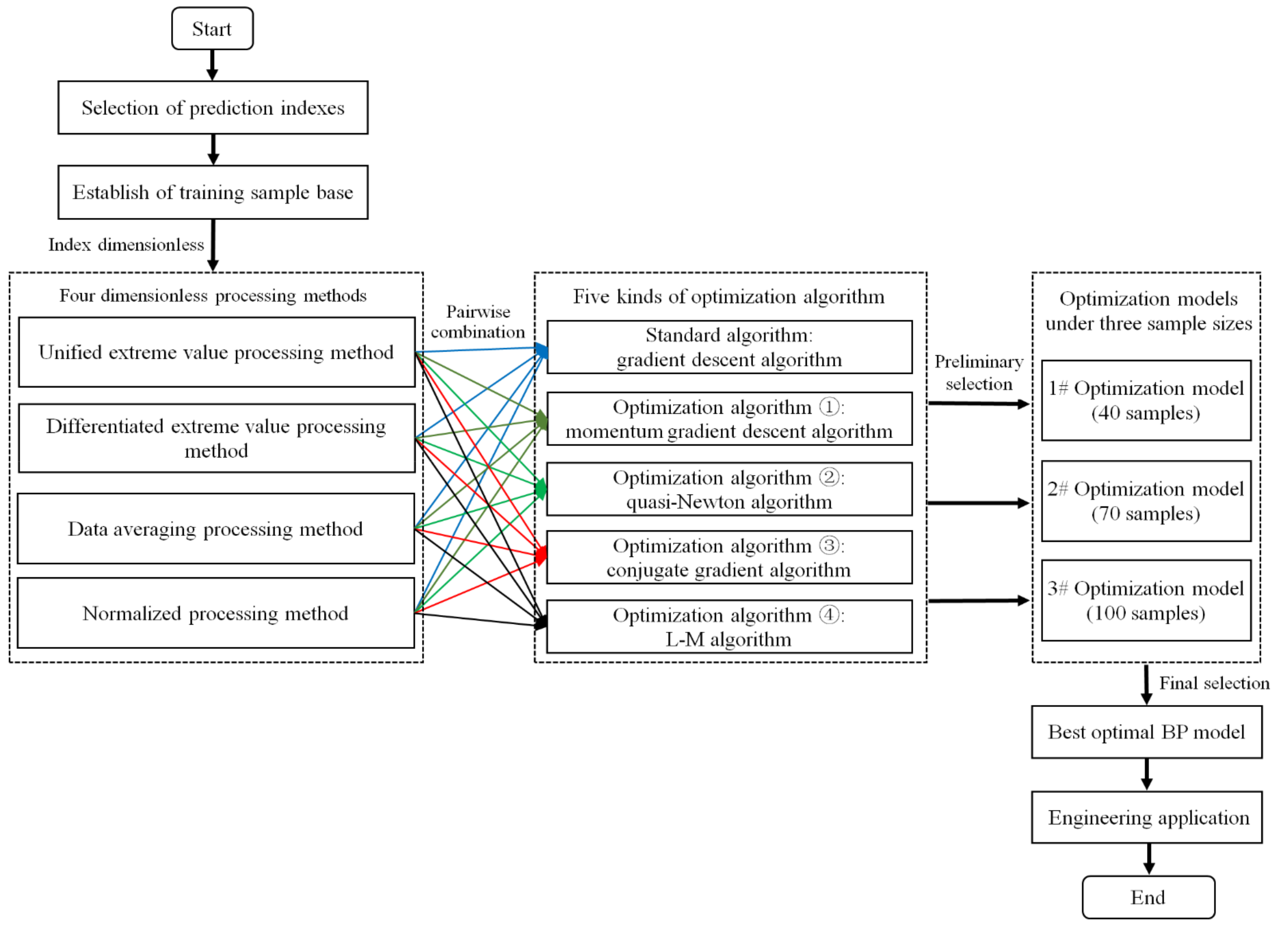
2.1. Dimensionless Methods
- (1)
- Unified extreme value processing method
- (2)
- Differentiated extreme value processing method
- (3)
- Data averaging processing method
- (4)
- Normalized processing method
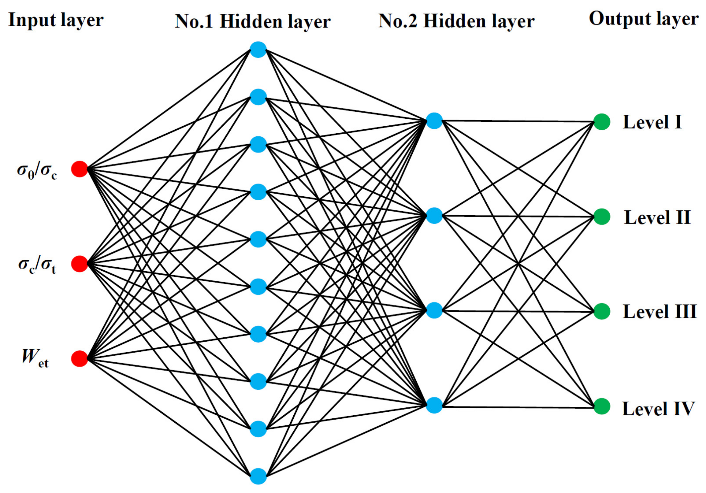
2.2. BP Neural Network
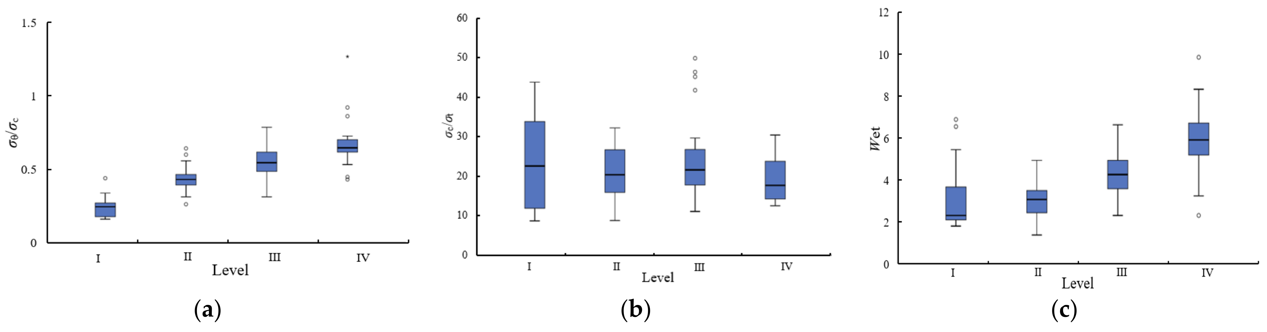
3. Index Selection and Data Analysis
4. Research Method
5. Prediction Results and Analysis
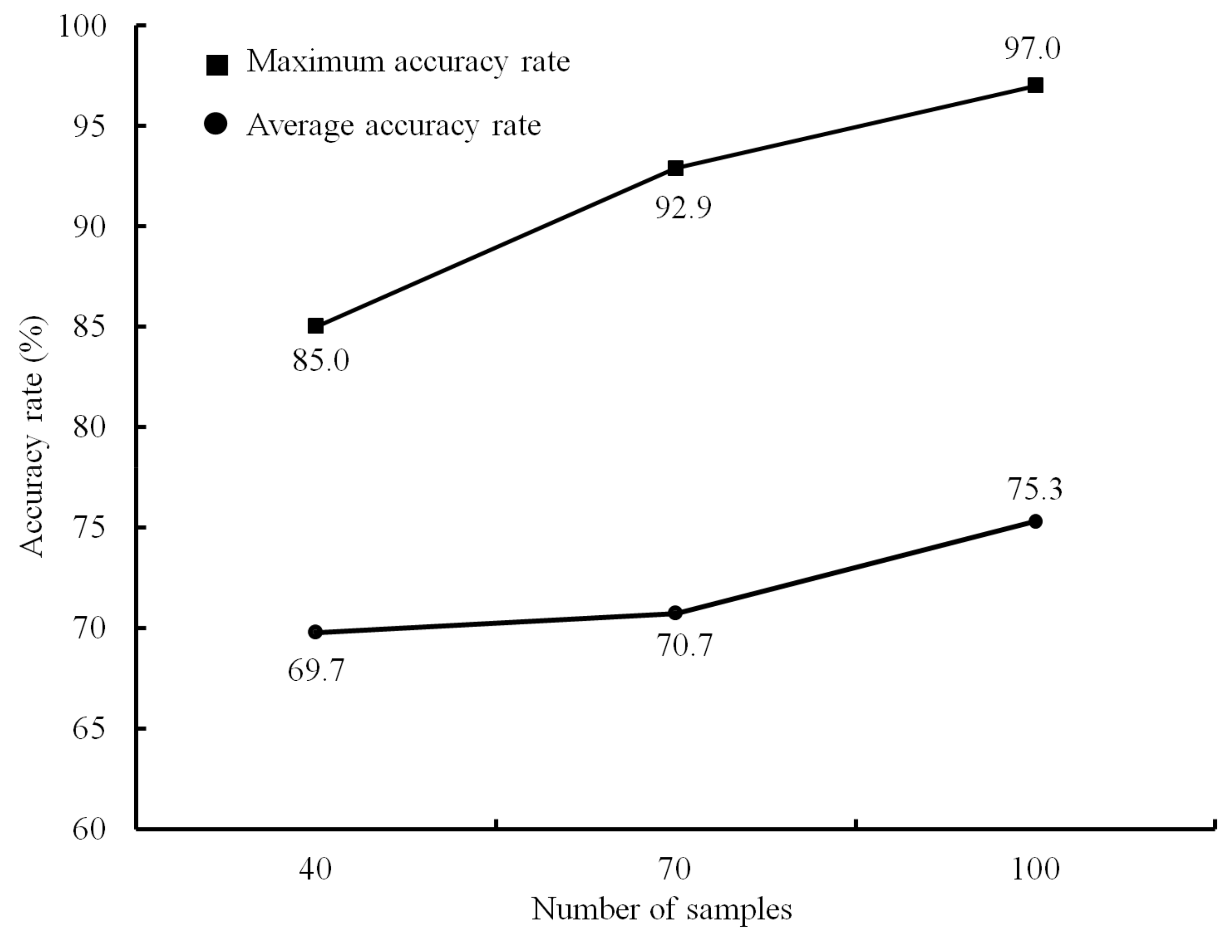
5.1. Prediction Results
5.2. Analysis
5.3. Limitation
6. Engineering Application
- (1)
- Maluping mine
- (2)
- Dongguashan copper mine
- (3)
- 3 + 390 working face of Jinping II hydropower station
7. Conclusions
Author Contributions
Funding
Institutional Review Board Statement
Informed Consent Statement
Data Availability Statement
Conflicts of Interest
Appendix A

| No. | Prediction Indexes | Actual Risk Level | ||
|---|---|---|---|---|
| σθ/σc | σc/σt | Wet | ||
| 1 | 0.11 | 31.2 | 7.4 | I |
| 2 | 0.10 | 23.0 | 5.7 | I |
| 3 | 0.20 | 36.0 | 2.3 | I |
| 4 | 0.19 | 47.9 | 1.9 | I |
| 5 | 0.13 | 6.7 | 1.4 | I |
| 6 | 0.19 | 6.7 | 1.4 | I |
| 7 | 0.23 | 6.7 | 1.4 | I |
| 8 | 0.28 | 9.7 | 1.9 | I |
| 9 | 0.11 | 27.2 | 7.0 | I |
| 10 | 0.13 | 18.8 | 3.6 | I |
| 11 | 0.10 | 21.4 | 4.7 | I |
| 12 | 0.31 | 42.8 | 1.8 | I |
| 13 | 0.20 | 11.2 | 3.6 | I |
| 14 | 0.20 | 14.1 | 3.6 | I |
| 15 | 0.28 | 42.7 | 2.2 | I |
| 16 | 0.11 | 29.4 | 2.0 | I |
| 17 | 0.23 | 7.5 | 1.5 | I |
| 18 | 0.43 | 45.9 | 1.7 | I |
| 19 | 0.22 | 36.4 | 1.8 | I |
| 20 | 0.40 | 15.6 | 3.5 | II |
| 21 | 0.44 | 13.1 | 2.1 | II |
| 22 | 0.37 | 24.0 | 5.1 | II |
| 23 | 0.45 | 11.2 | 2.0 | II |
| 24 | 0.67 | 26.8 | 0.9 | II |
| 25 | 0.56 | 20.4 | 2.0 | II |
| 26 | 0.46 | 20.4 | 2.0 | II |
| 27 | 0.49 | 19.7 | 2.3 | II |
| 28 | 0.44 | 19.7 | 2.3 | II |
| 29 | 0.42 | 19.7 | 2.3 | II |
| 30 | 0.46 | 19.7 | 2.3 | II |
| 31 | 0.28 | 23.6 | 4.9 | II |
| 32 | 0.56 | 34.3 | 1.9 | II |
| 33 | 0.30 | 20.4 | 5.0 | II |
| 34 | 0.35 | 22.7 | 3.3 | II |
| 35 | 0.45 | 14.8 | 3.1 | II |
| 36 | 0.41 | 30.7 | 4.3 | II |
| 37 | 0.22 | 9.0 | 4.9 | II |
| 38 | 0.45 | 6.8 | 2.2 | II |
| 39 | 0.35 | 12.1 | 2.9 | II |
| 40 | 0.37 | 29.7 | 3.5 | II |
| 41 | 0.42 | 32.8 | 3.0 | II |
| 42 | 0.38 | 28.8 | 3.0 | II |
| 43 | 0.62 | 8.3 | 1.8 | II |
| 44 | 0.42 | 29.9 | 2.4 | II |
| 45 | 0.42 | 15.5 | 3.2 | II |
| 46 | 0.57 | 31.2 | 3.2 | II |
| 47 | 0.34 | 24.0 | 6.6 | III |
| 48 | 0.42 | 21.7 | 5.0 | III |
| 49 | 0.40 | 14.7 | 7.1 | III |
| 50 | 0.40 | 15.0 | 7.1 | III |
| 51 | 0.48 | 24.0 | 5.1 | III |
| 52 | 0.61 | 24.0 | 5.1 | III |
| 53 | 0.70 | 11.7 | 2.8 | III |
| 54 | 0.83 | 28.9 | 3.2 | III |
| 55 | 0.74 | 28.9 | 3.2 | III |
| 56 | 0.79 | 22.0 | 2.0 | III |
| 57 | 0.84 | 19.7 | 2.3 | III |
| 58 | 0.52 | 21.2 | 5.5 | III |
| 59 | 0.60 | 28.3 | 3.4 | III |
| 60 | 0.53 | 21.0 | 3.6 | III |
| 61 | 0.66 | 21.5 | 4.1 | III |
| 62 | 0.52 | 17.8 | 4.3 | III |
| 63 | 0.57 | 25.6 | 3.8 | III |
| 64 | 0.61 | 25.6 | 3.7 | III |
| 65 | 0.56 | 29.2 | 4.8 | III |
| 66 | 0.49 | 49.5 | 4.7 | III |
| 67 | 0.46 | 45.5 | 5.2 | III |
| 68 | 0.47 | 55.0 | 5.0 | III |
| 69 | 0.61 | 25.0 | 3.7 | III |
| 70 | 0.55 | 31.3 | 4.6 | III |
| 71 | 0.50 | 50.9 | 5.2 | III |
| 72 | 0.69 | 16.9 | 3.4 | III |
| 73 | 0.54 | 12.2 | 4.9 | III |
| 74 | 0.47 | 16.5 | 5.5 | III |
| 75 | 0.52 | 18.6 | 4.2 | III |
| 76 | 0.55 | 11.1 | 4.0 | III |
| 77 | 0.56 | 16.3 | 3.3 | III |
| 78 | 0.28 | 9.5 | 6.1 | III |
| 79 | 0.66 | 22.3 | 3.2 | III |
| 80 | 0.72 | 27.5 | 4.3 | III |
| 81 | 0.62 | 19.4 | 4.5 | III |
| 82 | 0.59 | 18.8 | 4.2 | III |
| 83 | 0.77 | 17.5 | 5.5 | IV |
| 84 | 0.54 | 14.2 | 6.2 | IV |
| 85 | 0.58 | 13.2 | 6.3 | IV |
| 86 | 0.66 | 13.2 | 6.8 | IV |
| 87 | 0.74 | 24.4 | 6.3 | IV |
| 88 | 1.00 | 11.2 | 2.0 | IV |
| 89 | 0.93 | 28.9 | 3.2 | IV |
| 90 | 1.41 | 19.2 | 3.1 | IV |
| 91 | 0.71 | 32.2 | 5.5 | IV |
| 92 | 0.69 | 32.1 | 5.9 | IV |
| 93 | 0.42 | 17.0 | 10.9 | IV |
| 94 | 0.72 | 13.9 | 9.1 | IV |
| 95 | 0.64 | 14.4 | 7.7 | IV |
| 96 | 0.72 | 13.2 | 5.2 | IV |
| 97 | 0.65 | 28.6 | 6.8 | IV |
| 98 | 0.44 | 20.3 | 8.1 | IV |
| 99 | 0.64 | 17.5 | 7.2 | IV |
| 100 | 0.65 | 12.4 | 5.4 | IV |
References
- Zhao, J.; Jiang, Q.; Lu, J.F.; Chen, B.R.; Pei, S.F.; Wang, Z.L. Rock fracturing observation based on microseismic monitoring and borehole imaging: In situ investigation in a large underground cavern under high geo-stress. Tunn. Undergr. Space Technol. 2022, 126, 104549. [Google Scholar] [CrossRef]
- Zhao, J.; Jiang, Q.; Pei, S.; Chen, B.; Xu, D.P.; Song, L.B. Microseismicity and focal mechanism of blasting-induced block falling of intersecting chamber of large underground cavern under high geostress. J. Cent. South Univ. 2023, 30. [Google Scholar] [CrossRef]
- Du, W. Research on the law of geological disasters and prevention and control measures of tunnel excavation. D. Cent. South Univ. 2001.
- Adoko, A.; Gokceoglu, C.; Wu, L.; Zuo, Q. Knowledge-based and data-driven fuzzy modeling for rockburst prediction. Int. J. Rock Mech. Min. Sci. 2013, 61, 86–95. [Google Scholar] [CrossRef]
- Li, Y.; Wang, C.; Xu, J.; Zhou, Z.; Xu, J.; Cheng, J. Rockburst prediction based on the KPCA-APSO-SVM model and its engineering application. Shock. Vib. 2021, 2021, 7968730. [Google Scholar] [CrossRef]
- Li, X.; Eunhye, K.; Gabriel, W. A study of rock pillar behaviors in laboratory and in-situ scales using combined finite-discrete element method models. Int. J. Rock Mech. Min. Sci. 2019, 118, 21–32. [Google Scholar] [CrossRef]
- Zhou, J.; Li, X.; Shi, X. Long-term prediction model of rockburst in underground openings using heuristic algorithms and support vector machines. Saf. Sci. 2012, 50, 629–644. [Google Scholar] [CrossRef]
- Pu, Y.; Apel, D.; Xu, H. Rockburst prediction in kimberlite with unsupervised learning method and support vector classifier. Tunn. Undergr. Space Technol. 2019, 90, 12–18. [Google Scholar] [CrossRef]
- Faradonbeh, R.; Taheri, A. Long-term prediction of rockburst hazard in deep underground openings using three robust data mining techniques. Eng. Comput. 2019, 35, 659–675. [Google Scholar] [CrossRef]
- Yin, X.; Liu, Q.; Pan, Y.; Huang, X.; Wu, J.; Wang, X. Strength of stacking technique of ensemble learning in rockburst prediction with imbalanced data: Comparison of eight single and ensemble models. Nat. Resour. Res. 2021, 30, 1795–1815. [Google Scholar] [CrossRef]
- Dong, L.; Li, X.; Peng, K. Prediction of rockburst classification using random forest. Trans. Nonferrous. Met. Soc. China 2013, 23, 472–477. [Google Scholar] [CrossRef]
- Liang, W.; Sari, A.; Zhao, G.; McKinnon, D.; Wu, H. Short-term rockburst risk prediction using ensemble learning methods. Nat. Hazards 2020, 104, 1923–1946. [Google Scholar] [CrossRef]
- Liu, J.; Shi, H.; Wang, R.; Si, Y.; Wei, D.; Wang, Y. Quantitative risk assessment for deep tunnel failure based on normal cloud model: A case study at the Ashele copper mine, China. Appl. Sci. 2021, 11, 5208. [Google Scholar] [CrossRef]
- Lin, Y.; Zhou, K.; Li, J. Application of cloud model in rockburst prediction and performance comparison with three machine learning algorithms. IEEE Access 2018, 6, 2839754. [Google Scholar]
- Li, T.; Li, Y.; Yang, X. Rockburst prediction based on genetic algorithms and extreme learning machine. J. Cent. South Univ. 2017, 24, 2105–2113. [Google Scholar] [CrossRef]
- Xue, Y.; Bai, C.; Qiu, D.; Kong, F.; Li, Z. Predicting rockburst with database using particle swarm optimization and extreme learning machine. Tunn. Undergr. Space Technol. 2020, 98, 103287. [Google Scholar] [CrossRef]
- Sousa, L.; Miranda, T.; Sousa, R.; Tinoco, J. The use of data mining techniques in rockburst risk assessment. Engineering 2017, 3, 552–558. [Google Scholar] [CrossRef]
- Li, N.; Feng, X.; Jimenez, R. Predicting rockburst hazard with incomplete data using Bayesian networks. Tunn. Undergr. Space Technol. 2017, 61, 61–70. [Google Scholar] [CrossRef]
- Pu, Y.; Apel, D.; Lingga, B. Rockburst prediction in kimberlite using decision tree with incomplete data. J. Sustain. Min. 2018, 17, 158–165. [Google Scholar] [CrossRef]
- Ghasemi, E.; Gholizadeh, H.; Adoko, A. Evaluation of rockburst occurrence and intensity in underground structures using decision tree approach. Eng. Comput. 2020, 36, 213–225. [Google Scholar] [CrossRef]
- Faradonbeh, R.; Haghshenas, S.; Taheri, A.; Mikaeil, R. Application of self-organizing map and fuzzy c-mean techniques for rockburst clustering in deep underground projects. Neural Comput. Appl. 2019, 32, 8545–8559. [Google Scholar] [CrossRef]
- Afraei, S.; Shahriar, K.; Madani, H. Statistical assessment of rockburst potential and contributions of considered predictor variables in the task. Tunn. Undergr. Space Technol. 2018, 72, 250–271. [Google Scholar] [CrossRef]
- Ding, X.; Wu, J.; Li, J.; Liu, C. Artificial neural network for forecasting and classification of rockbursts. J. Hohai Univ. Nat. Sci. 2003, 31, 424–427. [Google Scholar]
- Guo, L.; Wu, A.; Ma, D. The method to predict rockbursts proneness based on RES theory. J. Cent. South Univ. Nat. Sci. 2004, 35, 304–309. [Google Scholar] [CrossRef]
- Bai, M.; Wang, L.; Xu, Z. Study on a neutral network model and its application in predicting the risk of rock blast. China Saf. Sci. J. 2002, 12, 65–69. [Google Scholar]
- Li, Y.; Yin, J.; Ai, K. Application of BP neural network in prediction of rockburst. J. Yangtze River Sci. Res. Inst. 2008, 25, 183–185+190. [Google Scholar] [CrossRef]
- Wang, B. Application of improved BP neural network in tunnel rockburst prediction. Transp. Stand 2010, 29, 86–89. [Google Scholar]
- Sun, C. A prediction model of rockburst in tunnel based on the improved MATLAB-BP neural network. J. Chongqing Jiaotong Univ. Nat. Sci. 2019, 38, 41–49. [Google Scholar]
- Zhang, Q.; Wang, W.; Liu, T. Prediction of rockbursts based on particle swarm optimization-BP neural network. J. China Three Gorges Univ. Nat. Sci. 2011, 33, 41–45+56. [Google Scholar]
- Hu, M.; Chen, J.; Lu, Y. Research on rockburst prediction based on BP neural network and GA. Min. Res. Dev. 2011, 31, 90–94. [Google Scholar]
- Meng, L.; Li, T.; Wang, Z. A model for predicting rockburst by MATLAB neural network toolbox. Chin. J. Geol. Hazard Control. 2003, 14, 81–85. [Google Scholar]
- Li, Y.; Wang, C.; Liu, Y. Classification of Coal Bursting Liability Based on Support Vector Machine and Imbalanced Sample Set. Minerals 2023, 13, 15. [Google Scholar] [CrossRef]
- Ahmad, M.; Hu, J.; Hadzima, M.; Ahmad, F.; Tang, X.; Rahman, Z.; Nawaz, A.; Abrar, M. Rockburst hazard prediction in underground projects using two intelligent classification techniques: A comparative study. Symmetry 2021, 13, 632. [Google Scholar] [CrossRef]
- Wu, S.; Wu, Z.; Zhang, C. Rockburst prediction probability model based on case analysis. Tunn. Undergr. Space Technol. 2019, 93, 103069. [Google Scholar] [CrossRef]
- Kornowski, J.; Kurzeja, J. Prediction of rockburst probability given seismic energy and factors defined by the expert method of hazard evaluation (MRG). Acta Geophys. 2012, 60, 472–486. [Google Scholar] [CrossRef]
- Wang, C.; Li, Y.; Zhang, C. Prediction model of rockburst intensity classification based on data mining analysis with large samples. J. Kunming Univ. Sci. Technol. Nat. Sci. 2020, 45, 26–31. [Google Scholar]
- Wang, C.; Li, Y.; Shao, L.; Zhang, Y.; Xu, J.; Wang, H. BP model for rockburst prediction based on nine unconstrained optimization algorithms is preferred. J. Kunming Univ. Sci. Technol. Nat. Sci. 2021, 46, 32–37. [Google Scholar]
- Liu, K.; Li, X.; Zhu, Z.; Brand, L.; Wang, H. Factor-bounded nonnegative matrix factorization. ACM Trans. Knowl. Discov. Data (TKDD) 2021, 15, 1–18. [Google Scholar] [CrossRef]
- Li, X.; Wang, H. Adaptive Principal Component Analysis. In Proceedings of the 2022 SIAM International Conference on Data Mining (SDM). Society for Industrial and Applied Mathematics, Alexandria, VA, USA, 28–30 April 2022. [Google Scholar]
- Yang, J.; Li, X.; Zhou, Z.; Lin, Y. A fuzzy assessment method of rock-burst prediction based on rough set theory. Met. Mine 2010, 39, 26–29. [Google Scholar]
- Tian, R.; Meng, H.; Chen, S.; Wang, C.; Zhang, F. Prediction of intensity classification of rockburst based on deep neural network. J. China Coal. Soc. 2020, 45, 191–201. [Google Scholar]
- Wang, Y.; Shang, Y.; Sun, H.; Yan, X. Study of prediction of rockburst intensity based on efficacy coefficient method. Rock Soil Mech. 2010, 31, 529–534. [Google Scholar]


| Level | Characteristic | σθ/σc | σc/σt | Wet |
|---|---|---|---|---|
| I | mean | 0.20 | 24.49 | 2.99 |
| median | 0.20 | 23.00 | 2.00 | |
| minimum | 0.10 | 6.70 | 1.40 | |
| maximum | 0.43 | 47.90 | 7.40 | |
| standard deviation | 0.20 | 36.00 | 2.30 | |
| II | mean | 0.43 | 20.77 | 2.94 |
| median | 0.42 | 20.40 | 2.90 | |
| minimum | 0.22 | 6.80 | 0.90 | |
| maximum | 0.67 | 34.30 | 5.10 | |
| standard deviation | 0.37 | 24.00 | 5.10 | |
| III | mean | 0.57 | 24.20 | 4.41 |
| median | 0.56 | 21.85 | 4.30 | |
| minimum | 0.28 | 9.50 | 2.00 | |
| maximum | 0.84 | 55.00 | 7.10 | |
| standard deviation | 0.40 | 14.70 | 7.10 | |
| IV | mean | 0.72 | 19.08 | 6.18 |
| median | 0.68 | 17.25 | 6.25 | |
| minimum | 0.42 | 11.20 | 2.00 | |
| maximum | 1.41 | 32.20 | 10.90 | |
| standard deviation | 0.58 | 13.20 | 6.30 |
| Prediction Model | Index Dimensionless Method | A (40)/% | A (70)/% | A (100)/% |
|---|---|---|---|---|
| Standard BP model | Unified extreme value processing method | 70.0 | 60.0 | 75.0 |
| Differential extreme value processing method | 77.5 | 48.6 | 59.0 | |
| Normalized processing method | 67.5 | 67.1 | 60.0 | |
| Data averaging processing method | 70.0 | 52.9 | 68.0 | |
| GDM–BP model | Unified extreme value processing method | 62.5 | 57.1 | 69.0 |
| Differential extreme value processing method | 52.5 | 60.0 | 69.0 | |
| Normalized processing method | 67.5 | 54.3 | 62.0 | |
| Data averaging processing method | 67.5 | 57.1 | 66.0 | |
| BFG–BP model | Unified extreme value processing method | 72.5 | 70.0 | 89.0 |
| Differential extreme value processing method | 65.0 | 70.0 | 81.0 | |
| Normalized processing method | 65.0 | 88.6 | 64.0 | |
| Data averaging processing method | 85.0 | 65.7 | 91.0 | |
| SCG–BP model | Unified extreme value processing method | 80.0 | 82.9 | 95.0 |
| Differential extreme value processing method | 77.5 | 81.4 | 78.0 | |
| Normalized processing method | 60.0 | 70.0 | 45.0 | |
| Data averaging processing method | 65.0 | 70.0 | 91.0 | |
| LM–BP model | Unified extreme value processing method | 80.0 | 92.9 | 97.0 |
| Differential extreme value processing method | 72.5 | 88.6 | 94.0 | |
| Normalized processing method | 70.0 | 84.3 | 58.0 | |
| Data averaging processing method | 67.5 | 92.9 | 95.0 |
| Prediction Model | Unified Extreme Value Processing Method | Differentiated Extreme Value Processing Method | Normalized Processing Method | Data Averaging Processing Method |
|---|---|---|---|---|
| Standard BP model | 145 | 124 | 134 | 133 |
| GDM–BP model | 134 | 132 | 127 | 133 |
| BFG–BP model | 167 | 156 | 152 | 171 |
| SCG–BP model | 185 | 166 | 118 | 166 |
| LM–BP model | 194 | 185 | 145 | 187 |
| Prediction Model | Extreme Difference |
|---|---|
| Standard BP model | 21 |
| GDM–BP model | 7 |
| BFG–BP model | 19 |
| SCG–BP model | 67 |
| LM–BP model | 49 |
| Dimensionless Method | Extreme Difference |
|---|---|
| Unified extreme value processing | 60 |
| Differentiated extreme value processing | 51 |
| Normalized processing | 34 |
| Data averaging processing | 54 |
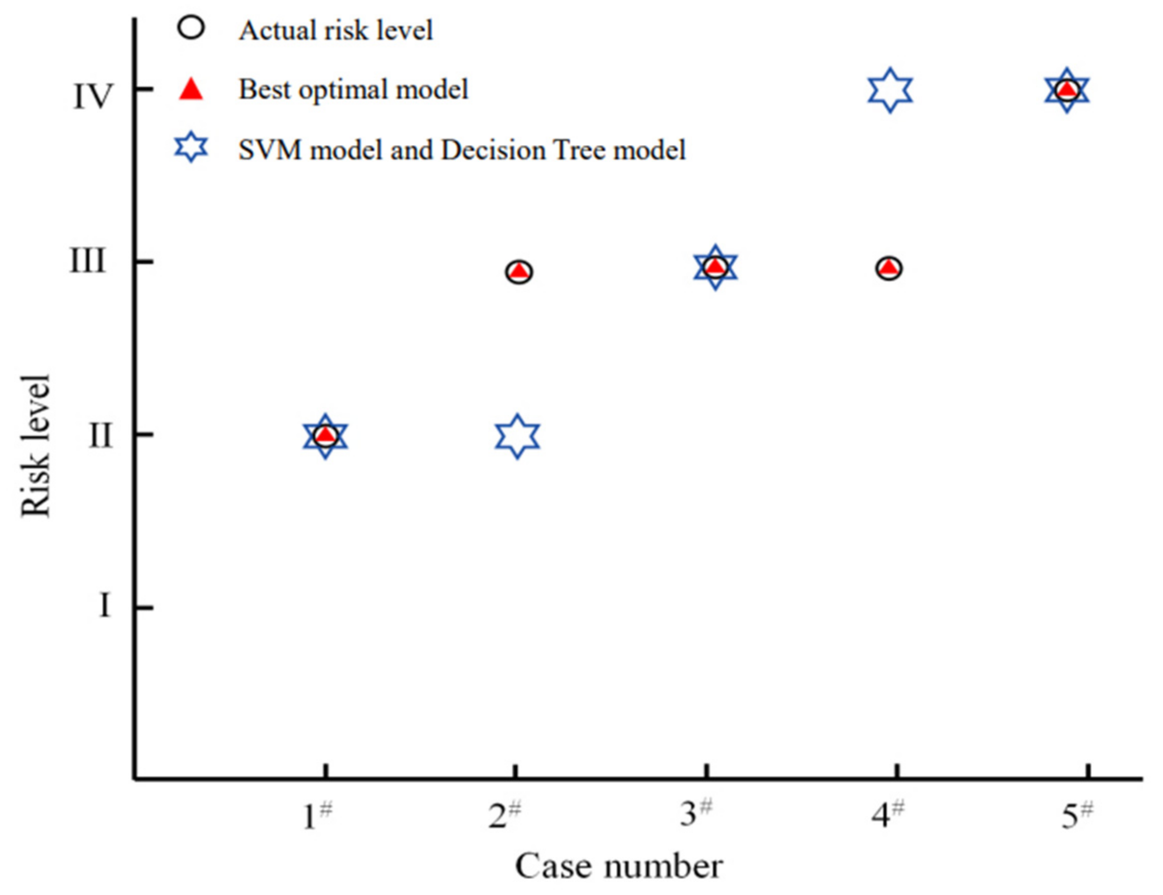
| No. | Prediction Indexes | Actual Level | Prediction Results | ||||
|---|---|---|---|---|---|---|---|
| σθ/σc | σc/σt | Wet | LM-BP Model | Decision Tree | SVM Model | ||
| 1 | 0.45 | 11.20 | 2.03 | II | II | II | II |
| No. | Prediction Indexes | Actual Level | Prediction Results | ||||||
|---|---|---|---|---|---|---|---|---|---|
| σθ/σc | σc/σt | Wet | LM-BP Model | Decision Tree | SVM Model | DA-DNN Model [41] | Cloud Model [41] | ||
| 2 | 0.46 | 11.10 | 3.97 | III | III | II | II | III | III |
| No. | Prediction Indexes | Actual Level | Prediction Results | |||||
|---|---|---|---|---|---|---|---|---|
| σθ/σc | σc/σt | Wet | LM-BP Model | Decision Tree | SVM Model | Cloud Model [42] | ||
| 3 | 0.84 | 19.69 | 2.30 | III | III | III | III | III |
| No. | Prediction Indexes | Actual Level | Prediction Results | ||||
|---|---|---|---|---|---|---|---|
| σθ/σc | σc/σt | Wet | LM-BP Model | Decision Tree | SVM Model | ||
| 4 | 0.42 | 13.98 | 7.44 | III | III | IV | IV |
| 5 | 0.65 | 28.60 | 6.80 | IV | IV | IV | IV |
Disclaimer/Publisher’s Note: The statements, opinions and data contained in all publications are solely those of the individual author(s) and contributor(s) and not of MDPI and/or the editor(s). MDPI and/or the editor(s) disclaim responsibility for any injury to people or property resulting from any ideas, methods, instructions or products referred to in the content. |
© 2023 by the authors. Licensee MDPI, Basel, Switzerland. This article is an open access article distributed under the terms and conditions of the Creative Commons Attribution (CC BY) license (https://creativecommons.org/licenses/by/4.0/).
Share and Cite
Wang, C.; Xu, J.; Li, Y.; Wang, T.; Wang, Q. Optimization of BP Neural Network Model for Rockburst Prediction under Multiple Influence Factors. Appl. Sci. 2023, 13, 2741. https://doi.org/10.3390/app13042741
Wang C, Xu J, Li Y, Wang T, Wang Q. Optimization of BP Neural Network Model for Rockburst Prediction under Multiple Influence Factors. Applied Sciences. 2023; 13(4):2741. https://doi.org/10.3390/app13042741
Chicago/Turabian StyleWang, Chao, Jianhui Xu, Yuefeng Li, Tuanhui Wang, and Qiwei Wang. 2023. "Optimization of BP Neural Network Model for Rockburst Prediction under Multiple Influence Factors" Applied Sciences 13, no. 4: 2741. https://doi.org/10.3390/app13042741
APA StyleWang, C., Xu, J., Li, Y., Wang, T., & Wang, Q. (2023). Optimization of BP Neural Network Model for Rockburst Prediction under Multiple Influence Factors. Applied Sciences, 13(4), 2741. https://doi.org/10.3390/app13042741