Computer Percolation Models for Espresso Coffee: State of the Art, Results and Future Perspectives

Abstract

Coffee is one of the most consumed beverages in the world. This has two main consequences: a high level of competitiveness among the players operating in the sector and an increasing pressure from the supply chain on the environment. These two aspects have to be supported by scientific research to foster innovation and reduce the negative impact of the coffee market on the environment. In this paper, we describe a mathematical model for espresso coffee extraction that is able to predict the chemical characterisation of the coffee in the cup. Such a model has been tested through a wide campaign of chemical laboratory analyses on espresso coffee samples extracted under different conditions. The results of such laboratory analyses are compared with the simulation results obtained using the aforementioned model. The comparison shows a close agreement between the real and in silico extractions, revealing that the model is a very promising scientific tool to take on the challenges of the coffee market.

1. Introduction

Coffee needs no introduction, it is one of the most consumed beverages around the world. Its supply chain involves almost all countries, from producers to roasters and consumers. Despite coffee production being limited to geographical areas with favourable climate conditions, most countries have coffee consumers among their populations [1], and each country uses its preferred extraction techniques. The reasons for fostering coffee consumption are various and depend on the consumer’s feelings or needs. In fact, coffee is a multi-purpose beverage with its functional, social and healthy benefits. As a consequence, one of the main future goals of the coffee industry is the customised coffee preparation, because personal preferences are influenced by people’s traditions and culture but also depend on temporary needs and health issues. For instance, a strong coffee usually aids concentration after a poor night’s sleep or a light drink is usually sought after a heavy meal.

Different coffee brews have been characterised by several chemical studies. Many of those are devoted to the extraction of espresso coffee (EC) and its peculiarity, because EC is a complex beverage, poorly stable with respect to volatiles and foam and unique in its sensorial properties. In fact, it is described as a beverage with a heavy body, intense aroma, bitter/acid taste and pleasant lingering aftertaste [2]. More than 1000 compounds occur in a cup of EC, among them caffeine is the best-known compound and its recognition and attraction are probably due to the stimulating effects on the central nervous system [3]. Caffeine also influences the coffee flavour since, together with other compounds, such as trigonelline, thermally generated compounds (e.g., pyrazines, piperazine) and derivatives of phenolic acids (e.g., chlorogenic acid), it affects the bitterness of coffee. The bitterness is an important attribute of EC that drives consumer acceptance [4]. In addition, several pieces of evidence have demonstrated that phenolic acids and chlorogenic acids possess antioxidant, anti-inflammatory and anticarcinogenic activities [5,6,7]. Another revered taste of coffee flavour is the acidity (sourness); organic acids, such as acetic, citric and tartaric acid, seem to be the main responsible for this sensation in the oral mucosa [8]. Regarding aroma, lipids play a key role because they retain lipophilic compounds that sensibly contribute to the aroma of the beverage. Numerous factors, such as type of coffee blend, roasting and grinding degree and preparation method (i.e., coffee extraction technique) can influence the levels of chemical compounds that arrive in the cup and, accordingly, the final coffee flavour and quality [9,10]. Therefore, a study that brings together all the mentioned compounds provides an all-round description of a cup of coffee, in terms of flavour, quality and health-related aspects.

The chemical and physical aspects in coffee extraction are complex, thus a complete description of such a process by a mathematical model is challenging. The physico-chemical modelling of coffee extraction has been faced in a limited number of studies. Among them, the model provided in [11] uses an approach that deals with the intragranular and intergranular motion of coffee particles to illustrate the dissolution and transport of filtered coffee. This one-dimensional model has been exploited in [12] to study the coffee extraction uniformity. In [13], a one-dimensional percolation model is proposed and used to calculate the Extraction Yield (EY), i.e., an important indicator used by the coffee industry to describe the extraction efficiency. A similar percolation model is used in [14] to predict the EY and the proposed numerical approach ensures the positivity of the concentrations and the mass conservation. The same solving strategy is also adopted in [15] where the percolation model is generalised for the prediction of an arbitrary number of chemical compounds. All these one-dimensional percolation models have the advantage to be simple computational tools to predict the global water flow and extraction dynamics, considering quantities averaged over the whole domain or over some domain sections [16]. The only three-dimensional model, considering the main percolation processes and endowed with numerical simulations and a preliminary experimental validation, can be found in [17].

In this paper, we investigate the EC extraction process by a mathematical model to characterise an espresso beverage through the identification of the nutritional and organoleptic characteristics. Such a study enlarges and completes the model proposed in [17], introducing the dynamics of all the most important compounds in a coffee cup, considering wide extraction conditions, different granulometries of the coffee powder and different coffee varieties. In particular, we analyse a detailed physico-chemical model of water percolation in a porous medium to compute the amount of each chemical compound at the end of the extraction process with prescribed geometrical and physical parameters and the respective initial concentrations in the coffee powder. This comprehensive model is experimentally validated on the basis of the comparison between the amount of compounds obtained by numerical simulations and the ones obtained from chemical laboratory analyses. To this purpose, a large extraction campaign has been conducted under different extraction conditions (water temperature and water pressure), physical characteristics of the coffee powder (granulometry) and coffee varieties. These extraction conditions have been recognised as critical aspects in coffee preparation, in fact, the scientific literature has extensively shown that these parameters significantly influence the chemical characterisation of a coffee cup [18,19,20]. In particular, among the extraction conditions considered, water temperature and pressure vary in their maximum admissible range for espresso extraction, whereas the tamping pressure is discarded as its influence in the chemical composition of the cup is hardly detectable [18]. Concerning the granulometry, three different particle size profiles are considered because the grain dimension influences both the extraction kinetics and the final chemical profile. The different granulometries are obtained starting from a reference granulometry, called optimal, which is the granulometry that allows one to obtain 40 g (gram) of coffee from 20 g of powder in 20 s (second). Then, finer and coarser granulometries with respect to the optimal one are obtained with the empirical rule of keeping the amount of extracted coffee but increasing and decreasing the extraction time, respectively. As far as coffee varieties are concerned, the choice falls on the extremes, i.e., the Arabica and Robusta varieties, for two reasons: the speciality coffee world commonly performs single variety coffee extractions and, on the other hand, it is assumed that some linear interpolation of the results can be performed to characterise a blend of Arabica and Robusta. The obtained interesting results pave the way towards the rigorous analysis of two ambitious applications: 1. the customisation of the coffee beverage by devising a relation between chemical compounds and taste; 2. the study of innovative extraction techniques. Such applications cannot be investigated through simplified percolation models, which do not give precise predictive power on the extraction dynamics for each chemical compound. Conversely, the proposed model is able to address some lack of symmetry in the domain (for instance, extractions by using filters without cylindrical symmetry) or to be easily generalised to more complex processes, such as the centrifuge extraction [21].

The paper is organised as follows. Section 2 describes the materials and methods used in this research, in particular, both the water percolation model in a porous medium and the procedures for the chemical analyses. Section 3 reports and discuss both the results of the laboratory analyses and the results of the numerical simulations. From the laboratory results, a direct connection can be understood between chemical compounds in the coffee cup and physico-chemical variables involved in the extraction. In addition, Section 3 compares the laboratory measurements with the numerical results. Finally, Section 4 gives some closing comments and further developments.

2. Materials and Methods

The materials and methodologies used to carry out this research are described. In particular, Section 2.1 briefly describes the fluid-dynamics model in a porous medium that formulates the percolation process. Section 2.2 presents the materials used and procedures followed in the chemical laboratory analyses performed both on the EC and the ground coffee samples.

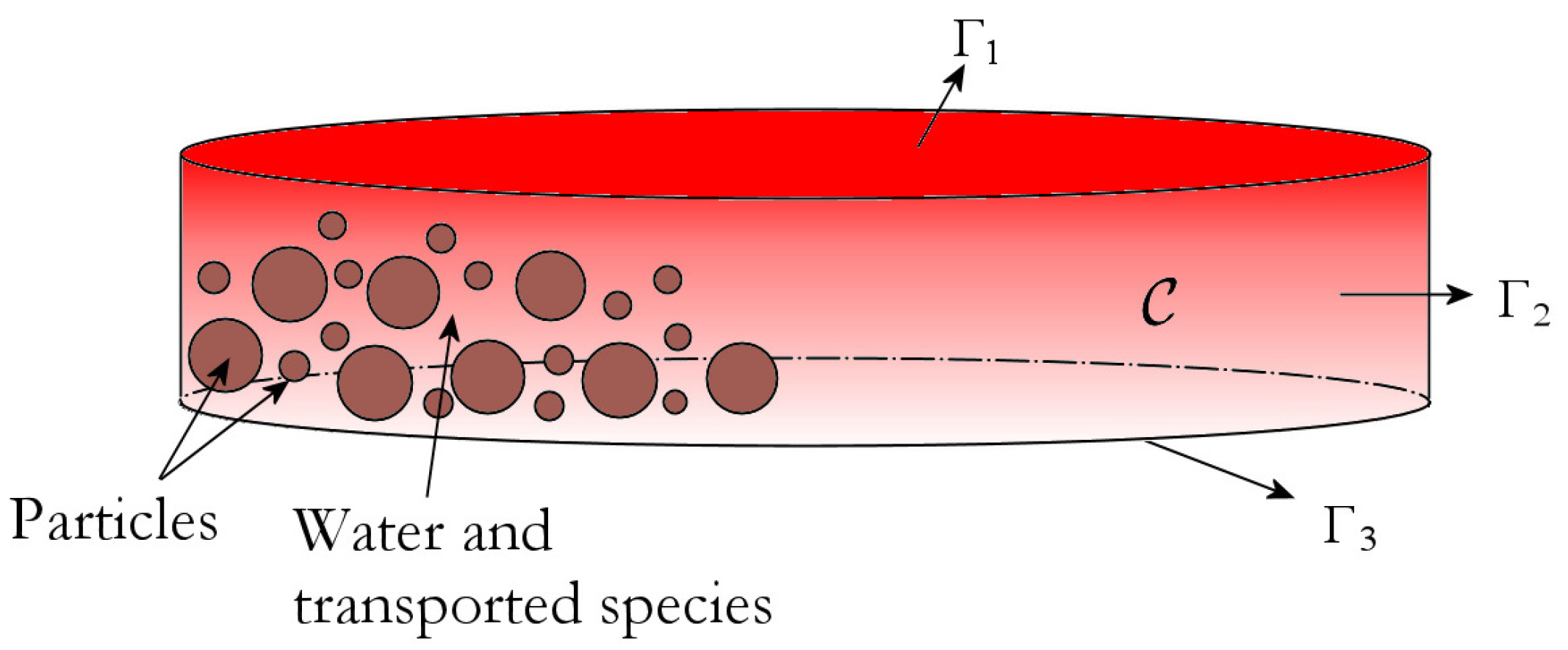
2.1. The Percolation Model

The EC extraction consists of the following physico-chemical process: hot water with prescribed pressure pours into the basket and hits the tamped coffee powder within the basket, it flows into the powder passing by the void spaces in the coffee grains and dissolves several chemical substances from the wet grains of the coffee pod. The water also removes a certain amount of fine particles from the ground coffee and transports it downward. This extraction process can be described as a fluid-dynamics process that is the well-known percolation process. From the fluid-dynamics point of view, these components are involved: the dynamics of the fluid, the fine particles worn away by the flow from the porous matrix and the chemical species dissolved in the fluid, as well as the transfer of heat between the solid medium and the fluid. The books [22,23] provide a general formalisation of percolation processes. A preliminary study of the percolation model used in this work can be found in [17]. This model is based on some key hypotheses:

• The porous medium is isotropic and homogeneous.
• A chemical species is called liquid if it undergoes the transport process; in contrast, a chemical species is called solid if it is not involved in the transport process so it is bound to the porous medium. Thus, being liquid or solid is independent of the actual physical phase.
• The first 5 s of the real extraction process are called imbibition, when the porous medium gets wet. After imbibition, there is no gaseous phase in the porous medium, the porous medium is saturated and a local thermal balance occurs between coffee powder and water. The percolation process is investigated after imbibition.

The percolation problem has the circular cylinder $\mathcal{C}$ in Figure 1 as spatial domain. We fix a 3D Cartesian coordinate system and we suppose that the z-axis of such system and the symmetry axis of $\mathcal{C}$ coincide, ${\Gamma }_3$ with radius R lays on the plane $z=-H$ while ${\Gamma }_1$ lays on the plane $z=0$, thus the height of $\mathcal{C}$ is $H>0$. The following model describes the physico-chemical process of EC percolation, under the previous assumptions:

$$\left\{\begin{array}{c}{S}_0\frac{\partial h}{\partial t}+\nabla ·\mathbf{q}=Q\hfill \\ \mathbf{q}=-\mathbf{K}{f}_{\mu }·(\nabla h+\chi \mathbf{e})\hfill \\ \begin{array}{ccc}\epsilon \frac{\partial C_k}{\partial t}+\mathbf{q}·\nabla C_k+\nabla ·{\mathbf{j}}_k=R_k-C_{k}Q,\hfill & \hfill & k=1,\dots ,N_{l-s},\hfill \\ {\epsilon }_s\frac{\partial C_m^s}{\partial t}=R_m^s,\hfill & \hfill & m=1,\dots ,N_s,\hfill \end{array}\hfill \\ \left(\epsilon \rho c+{\epsilon }_s{\rho }^s{c}^s\right)\frac{\partial T}{\partial t}+\rho c\mathbf{q}·\nabla T-\nabla ·(\mathsf{\Lambda }·\nabla T)=H_e-\rho c\left(T-T_0\right)Q,\hfill \end{array}\right.$$

(1)

prescribing all the equations in the spatial domain $\mathcal{C}$ and for $t\in (0,\tau )$, with $\tau >0$ the percolation time. We note that the fluid flow in porous media that are saturated is described in (1) by the first equation, which combined with the second one, is known as Richards Equation [24], formulated for the unknown hydraulic head h. Here, $S_0$ is the specific storage coefficient and the term Q accounts for sources and/or sinks of liquid mass. h depends on the pressure head $\psi$ and the elevation z, more precisely, $h=\psi +z$, where $\psi =p/{\rho }_{0}g$, with g the gravity acceleration, ${\rho }_0$ a fluid mass density of reference and p the pressure. The second equation is the Darcy law for the unknown Darcy flux $\mathbf{q}$. Here, $\mathbf{e}$ is the coordinate unit vector ${(0,0,1)}^T$, $\mathbf{K}$ is the hydraulic conductivity tensor and $\chi ,f_{\mu }$ the buoyancy coefficient and the viscosity relation function, respectively, which account for the effects of temperature and pressure on density and viscosity. The third equation is the advective–diffusive–reactive equation written for the chemical species k with unknown mass concentration $C_k$. Such concentration $C_k$ can be solid or liquid, in particular, a species appears in this equation if it undergoes transport and diffusion processes. The equations of this kind are $N_{l-s}$, each equation is associated with one liquid–solid species to be considered. In these equations, $R_k$ in the right-hand side denotes the total reaction rate of the k-th species [25], $\epsilon$ is the porosity, the hydrodynamic diffusion-dispersion ${\mathbf{j}}_k$ is given by the Fick’s law:

$${\mathbf{j}}_k=-{\mathbf{D}}_k·\nabla C_k,$$

where the hydrodynamic dispersion tensor, ${\mathbf{D}}_k$, is defined as:

$$\begin{array}{cc}\hfill {\mathbf{D}}_k& =\left(\epsilon D_k+{\beta }_T^k\parallel \mathbf{q}\parallel \right)\mathit{I}+\left({\beta }_L^k-{\beta }_T^k\right)\frac{\mathbf{q}\otimes \mathbf{q}}{\parallel \mathbf{q}\parallel },\hfill \end{array}$$

(2)

where ${\beta }_T^k$ is the transverse dispersion coefficient, ${\beta }_L^k$ is the longitudinal dispersion coefficient, $D_k$ is the molecular diffusion coefficient, $\mathit{I}$ is the identity matrix and the symbol ⊗ denotes the tensor product. Mass balance for the species m becomes the fourth equation, where $C_m^s$ is the unknown concentration. Such species m is uniquely solid, meaning attached to the solid matrix, as suggested by the superscript s, thus it is not involved in the diffusion and transport processes. The equations of this kind are $N_s$, one for each solid species of interest. Here, for the m-th solid species $R_m^s$ denotes the total reaction rate and ${\epsilon }_s=1-\epsilon$ denotes the solid volume fraction. System (1) lastly shows the heat equation, where the unknown is the system temperature T and both the convective and diffusive heat transfer are considered. Here, in the right-hand-side $H_e$ accounts for all the internal sources and/or sinks of energy, $T_0$ is a reference temperature, $\rho c$ is the fluid volumetric heat capacity, ${\rho }^s{c}^s$ is the solid volumetric heat capacity and $\mathsf{\Lambda }$ is the tensor of thermal hydrodynamic conductivity, whose definition is similar to that of ${\mathbf{D}}_k$:

$$\begin{array}{cc}\hfill \mathsf{\Lambda }& =\left(\epsilon \mathrm{\Lambda }+{\epsilon }_s{\mathrm{\Lambda }}^s+\rho c{\gamma }_T\parallel \mathbf{q}\parallel \right)\mathit{I}+\rho c({\gamma }_L-{\gamma }_T)\frac{\mathbf{q}\otimes \mathbf{q}}{\parallel \mathbf{q}\parallel },\hfill \end{array}$$

(3)

where ${\gamma }_L$ and ${\gamma }_T$ are the thermal dispersion coefficients for the longitudinal and transverse directions, respectively, ${\mathrm{\Lambda }}^s$ is the thermal conductivity of the solid matrix and $\mathrm{\Lambda }$ is the thermal conductivity of the fluid.

Boundary and initial conditions are required to close system (1) and briefly discussed in the following. For the hydraulic head, the conditions are:

$$\left\{\begin{array}{ccc}h=h_{z0},\hfill & \hfill & \mathrm{on}{\mathsf{\Gamma }}_1,t>0,\hfill \\ \frac{\partial h}{\partial r}=0,\hfill & \hfill & \mathrm{on}{\mathsf{\Gamma }}_2,t>0,\hfill \\ \mathbf{q}·\mathbf{n}=-{\mathsf{\Phi }}_{h}min\{h_C-h,0\},\hfill & \hfill & \mathrm{on}{\mathsf{\Gamma }}_3,t>0,\hfill \\ p=p_0\left(z\right),\hfill & \hfill & \mathrm{in}\mathcal{C},t=0,\hfill \end{array}\right.$$

(4)

where the initial condition for h is missing due to the definition of the initial condition for p that automatically prescribes an initial condition for h. In (4), $p_0$ is the prescribed pressure profile when percolation starts, thus for the compatibility condition it must be $h_{z0}=p_0\left(0\right)/{\rho }_{0}g$. In these and the successive conditions where necessary, the outward unit normal vector is denoted by $\mathbf{n}$. Moreover, the third condition allows an external flux with rate ${\mathsf{\Phi }}_h(h-h_C)$ when $h>h_C$, where ${\mathsf{\Phi }}_h$ is a prescribed transfer coefficient that can be considered as the admittance of the filter placed at the lower base of the coffee pod, and $h_C$ is a proper value for the hydraulic head.

For the concentration $C_k$ of the k-th liquid/solid species, the following conditions are adopted:

$$\left\{\begin{array}{ccc}\nabla C_k·\mathbf{n}=0,\hfill & \hfill & \mathrm{on}{\mathsf{\Gamma }}_1,{\mathsf{\Gamma }}_2,t>0,\hfill \\ -({\mathbf{D}}_k·\nabla C_k)·\mathbf{n}=-{\mathsf{\Phi }}_{k}min\{C_{kC}-C_k,0\},\hfill & \hfill & \mathrm{on}{\mathsf{\Gamma }}_3,t>0,\hfill \\ C_k=0,\hfill & \hfill & \mathrm{in}\mathcal{C},t=0,\hfill \end{array}\right.$$

(5)

where, as before, the admittance of the filter is denoted by ${\mathsf{\Phi }}_k$ but in this case, it refers to the species k, and a proper value of the concentration $C_{kC}$ is defined. In such a way, when $C_k>C_{kC}$, an external mass flux occurs with rate ${\mathsf{\Phi }}_k(C_k-C_{kC})$. Moreover, on the top and lateral faces, a Neumann condition is prescribed because no further changes in the solution are considered beyond such faces.

On the other hand, only the initial condition is required for the solid species m:

$$\begin{array}{ccc}\hfill & C_m^s=C_0^s,\hfill & \hfill \mathrm{in}\mathcal{C},t=0,\end{array}$$

(6)

where the initial concentration of the species m in the solid fraction of the porous matrix is $C_0^s$.

Finally, for the temperature these conditions are prescribed:

$$\left\{\begin{array}{ccc}T=T_{z0},\hfill & \hfill & \mathrm{on}{\mathsf{\Gamma }}_1,t>0,\hfill \\ \nabla T·\mathbf{n}=0,\hfill & \hfill & \mathrm{on}{\mathsf{\Gamma }}_2,{\mathsf{\Gamma }}_3,t>0,\hfill \\ T=T_0,\hfill & \hfill & \mathrm{in}\mathcal{C},t=0,\hfill \end{array}\right.$$

(7)

where $T_0$ is the temperature of the thermally balanced system water-porous medium when the percolation starts, and $T_{z0}$ is the temperature of the water entering the coffee pod. At the lateral and bottom faces, the Neumann condition is imposed because the real profile of the temperature is unknown on those faces.

2.2. Chemical Analyses

Two types of coffee were selected for this study, i.e., Arabica and Robusta. Arabica coffee was a blend from Perfero caffè (Fermo, Italy) composed of 50% of natural coffee, Geisha from Peru, variety typica, caturra and 50% of natural coffee from Guatemala (Batch 12-221, Perfero caffè), with a medium roasting degree for EC. Robusta coffee was a blend from Perfero caffè constituted by 50% of Uganda coffee and 50% of Indonesia (Flores island) coffee (Batch 10-221, Perfero caffè), with a medium roasting degree for EC. For the present research, about 4 kg (kilogram) of coffee beans Arabica and 4 kg of Robusta have been used. Coffee beans were ground by Mythos 1 grinder (Simonelli Group S.p.A., Belforte del Chienti, Italy) [26], and the coffee powder was tamped by the automatic tamping machine PuqPress M2 [27]. The preparation of EC samples was performed by a professional barista using the VA388 Black Eagle espresso coffee machine from Victoria Arduino (Simonelli Group S.p.A.) [28]. The EC extraction was carried out by keeping constant the amount of coffee (20 ± 0.1 g) added in the VST^© Competition filter basket and the amount of EC obtained in the cup (40 ± 2 g). The tamping force (20 kgF—kilogram-force) was kept constant for each sample as well. Then, the experiment was focused on varying three extraction parameters, i.e., granulometry (O, optimal; C, coarse; F, fine), temperature of water (88, 93.4 and 98 °C) and pressure of water (6, 9 and 12 bar), resulting in a grid of 27 different EC samples for Arabica and 27 for Robusta. The time of extraction was fixed at 25 ± 1 s for EC samples considered optimal (optimal granulometry, water temperature of 93.4 °C and water pressure of 9 bar) and was different for EC samples prepared at different conditions than those optimal, since the brew ratio between mass of coffee pod and mass of EC was kept constant, 1:2. Moreover, another six EC samples were prepared by setting different conditions than those occurring in the previous grid. Hence, a total of 33 EC samples were prepared for Arabica and 33 for Robusta coffee.

Table 1. Extraction conditions of each EC sample. r denotes the type of granulometry: optimal (O), coarse (C) and fine (F).

Arabica Sample	T [°C]	p [bar]	r	Robusta Sample	T [°C]	p [bar]	r
A1	93.4	9	O	R1	93.4	9	O
A2	93.4	6	O	R2	93.4	12	O
A3	93.4	12	O	R3	93.4	6	O
A4	88	9	O	R4	88	9	O
A5	88	6	O	R5	88	12	O
A6	88	12	O	R6	88	6	O
A7	98	12	O	R7	98	9	O
A8	98	9	O	R8	98	12	O
A9	98	6	O	R9	98	6	O
A10	96	9	O	R10	96	9	O
A11	91	8	O	R11	91	8	O
A12	93.4	9	C	R12	93.4	9	C
A13	93.4	6	C	R13	93.4	12	C
A14	93.4	12	C	R14	93.4	6	C
A15	98	9	C	R15	88	9	C
A16	98	12	C	R16	88	12	C
A17	98	6	C	R17	88	6	C
A18	88	9	C	R18	98	9	C
A19	88	12	C	R19	98	12	C
A20	88	6	C	R20	98	6	C
A21	89	10	C	R21	97	7	C
A22	97	7	C	R22	89	10	C
A23	93.4	9	F	R23	93.4	9	F
A24	93.4	6	F	R24	93.4	12	F
A25	93.4	12	F	R25	93.4	6	F
A26	98	12	F	R26	88	9	F
A27	98	6	F	R27	88	12	F
A28	98	9	F	R28	88	6	F
A29	88	9	F	R29	98	6	F
A30	88	12	F	R30	98	9	F
A31	88	6	F	R31	98	12	F
A32	90	8	F	R32	95	11	F
A33	95	11	F	R33	90	8	F

summarises the extraction conditions for each EC sample. All the extractions were performed in duplicate ($n=2$).

The EC samples were analysed for the contents of total solids, total lipids and some selected bioactive compounds such as alkaloids (caffeine and trigonelline), chlorogenic acids (3-caffeoylquinic acid, 3-CQA, 5-caffeoylquinic acid, 5-CQA and 3,5-dicaffeoylquinic acid, 3,5-diCQA), phenolic acids (ferulic acid) and organic acids (acetic, citric and tartaric acid). These classes of compounds affect the coffee taste and flavour hence they participate at the final cup quality. The analysis of total lipids and contents of these different classes of compounds were also performed in roasted and ground (R&G) coffee for both Arabica and Robusta. Hence, the EY for each class of compounds was approximately estimated. All the performed analyses were carried out almost in duplicate ($n=2$) since the acceptable Relative Standard Deviation (% RSD) was fixed to 20%.

The materials and methods used in the laboratory analyses are illustrated in the following. In Section 2.2.1, all the chemicals and reagents are listed and their acquisition specified. In Section 2.2.2 and Section 2.2.3, the procedures for the analysis of total solids, lipids and bioactive compounds are described, respectively, both for the EC and R&G coffee powder.

2.2.1. Chemicals and Reagents

The analytical standards for each studied compound have been purchased from Sigma-Aldrich (Milan, Italy). Stock solutions of the alkaloids, phenolic acids and chlorogenic acids were prepared by dissolving the pure powder into methanol (10 mg/10 mL, where mg denotes milligram and mL millilitre), while those of organic acids by dissolving the pure powder into water (100 mg/10 mL). Working diluted solutions were daily prepared by appropriately diluting the stock solution in methanol or water (organic acids). Ultrapure water was obtained by purified deionised water by Milli-Q Reagent Water System (Bedford, MA, USA). Phosphoric acid ($H_{3}P{O}_4$, 85%) and HPLC-grade acetonitrile were bought from Sigma-Aldrich (Milan, Italy). All other chemicals and reagents were analytical grade. Before HPLC-DAD analysis, all samples were filtered by Captiva PTFE 13 mm (millimetre), 0.45 μm (micrometre) filter from Agilent Technology (Santa Clara, CA, USA).

2.2.2. Total Solids and Total Lipids

Total solids were measured by following the existing procedures but with some adjustments [29,30]. A total of 1 mL of the EC sample was oven dried up to constant weight (12 h, 100 ± 2 °C, where h denotes hours and °C degree Celsius). The remaining solid residue was measured and total solids were defined as the ratio between dry coffee residue and the volume of EC (w/v, i.e., weight/volume) expressed in g/100 mL.

Total lipids in EC samples were analysed by following already developed procedures but with some modifications [29,30]. Briefly, a liquid–liquid extraction with hexane (3 times, 5 mL) was performed from 10 mL of Arabica EC. For the Robusta samples, 20 mL of EC were extracted three times with 10 mL of hexane. Each time the organic phase was pipetted out and each fraction reconstituted into a flask. Then, sample was dried using anhydrous sodium sulfate, filtered and transferred into a round bottom flask. Finally, the solvent was removed by Buchi rotavapor R-200 (Buchi Italia s.r.l., Cornaredo, Italy) under reduced pressure. The total weight of lipids was measured after complete evaporation of solvent and total lipids were defined as the ratio between dry organic-phase residue and the volume of EC (w/v) expressed as g/100 mL.

The analysis of total lipids in R&G coffee has been carried out by following an existing procedure with some modifications [31]. A total of 55.5 g of R&G coffee were extracted with 500 mL of hexane (solvent-to-sample ratio, 9:1) in a Soxhlet extractor for 6.5 h. The liquid extract was then dried using anhydrous sodium sulfate, filtered and transferred into a round bottom flask. Using a Buchi rotavapor R-200, the solvent was evaporated and then the coffee oil residue weighed. Total solids in R&G coffee were expressed as g/100 g.

2.2.3. Bioactive Compounds Analysis by HPLC-DAD

The preparation method for bioactive compounds analysis such as alkaloids, chlorogenic acids, organic acids and phenolic acids in EC and R&G coffee was performed by following previous procedures [8,17]. Briefly, EC sample was diluted 1:50 in mobile phase, centrifuged at 13,000 rpm (revolutions per minute) for 10 min (minute) and filtered using 0.45 μm filter. In contrast, bioactive compounds from R&G coffee (1 g) were extracted with 20 mL of water at 80 °C for 30 min in a water bath under magnetic stirring. After cooling down the sample at room temperature, this was centrifuged for 5 min at 5000 rpm, diluted 1:5 in mobile phase and filtered with 0.45 μm filter.

The analysis of bioactive compounds has been performed by implementing an already developed analytical method [8]. In detail, the analysis has been carried out by using an Agilent 1100 series high-performance liquid chromatograph with a diode-array detector (DAD) from Agilent Technology (Santa Clara, CA) instead of an HPLC coupled with variable wavelength detector (VWD). In addition, in the current method other two chlorogenic acids have been added, i.e., 3-CQA and 3,5-diCQA. The separation of bioactive compounds was achieved onto Gemini C18 analytical column (250 mm × 3 mm × 5 μm) from Phenomenex (Castel Maggiore, Bologna, Italy). The mobile phase was composed of phosphate buffer solution (pH 2.5) (A) and acetonitrile (B). The elution has been achieved at 0.6 mL/min in gradient mode as follows: 0 min, 2% B; 5 min, 2% B; 10 min, 15% B; 15 min, 15% B; 18 min, 30% B, 23 min, 30% B; 25 min, 40% B. The injection volume was 5 μL and the temperature of the column was 30 °C. The acquisition was performed by monitoring a wavelength of 325 nm (nanometre) for chlorogenic acids and phenolic acids, 200 nm for organic acids, 264 nm and 274 nm for trigonelline and caffeine, respectively.

3. Results and Discussion

Results of the whole research are given and discussed, starting from the results obtained by the chemical laboratory analyses, given in Section 3.1; then, the numerical results are shown in Section 3.2, together with a comparison between such in silico results and the chemical ones from real extractions.

3.1. Results of Chemical Analyses

The results of chemical analyses are shown for all the different EC samples, reported in Table 1 and obtained with this extraction protocol: 20 ± 0.1 g in and 40 ± 2 g out. In Section 3.1.1, the results for total solids and lipids are presented, while in Section 3.1.2, the results for caffeine, trigonelline, cholorogenic acids, ferulic acid, acetic acid, citric acid and tartaric acid are shown.

3.1.1. Total Solids and Total Lipids: Results

Total solids, also called dry matter, measure the strength or concentration of coffee brew, which is the first indicator of coffee extraction efficiency [10]. In this study, total solids have been calculated in different EC samples prepared by varying granulometry, pressure and temperature using two coffee types, i.e., Arabica and Robusta. These results are shown in

Table 2. Content of total solids (TS) (g/100 mL) found in different EC samples, Arabica and Robusta.

Arabica Sample	TS (g/100 mL)	RSD (%)	Robusta Sample	TS (g/100 mL)	RSD (%)
A1	10.03	2.9	R1	9.78	17.9
A2	9.65	2.6	R2	10.12	16.9
A3	10.42	1.0	R3	10.15	18.8
A4	9.69	4.7	R4	10.31	9.7
A5	9.59	2.4	R5	10.72	9.1
A6	9.94	5.4	R6	11.20	0.9
A7	9.87	10.7	R7	11.19	3.8
A8	9.80	3.2	R8	9.63	14
A9	9.38	1.9	R9	10.88	3.7
A10	9.57	0.4	R10	12.09	16.9
A11	10.21	4.5	R11	9.83	14.5
A12	8.79	2.2	R12	9.46	3.6
A13	10.08	11.2	R13	8.62	17.1
A14	10.38	14.4	R14	10.86	0.7
A15	9.15	8.9	R15	9.69	4.7
A16	9.38	0.9	R16	11.03	5.6
A17	9.49	4.5	R17	9.13	2.7
A18	9.59	6.8	R18	9.53	1.8
A19	9.05	1.2	R19	8.85	19.4
A20	9.79	0.9	R20	11.30	8.0
A21	8.80	6.4	R21	10.88	11.0
A22	9.22	1.2	R22	8.53	9.6
A23	10.73	5.0	R23	12.55	3.5
A24	10.84	7.6	R24	10.05	18.3
A25	10.50	2.3	R25	11.95	6.7
A26	10.90	9.9	R26	11.63	18.6
A27	11.61	2.3	R27	11.28	3.1
A28	10.93	3.5	R28	10.36	3.5
A29	10.87	6.2	R29	12.37	8.3
A30	10.65	0.6	R30	11.23	0.3
A31	11.52	5.6	R31	11.73	13.7
A32	11.42	4.5	R32	10.90	13.8
A33	10.31	1.9	R33	11.19	3.7

.

ECs prepared with finer coffee powder generate higher levels of total solids (total solids average of all ECs prepared with coarse, optimal and fine granulometry, 9.52, 9.82 and 10.73 g/100 mL for Arabica and 9.83, 10.44 and 11.46 g/100 mL for Robusta, respectively). At optimal conditions, i.e., 9 bar of pressure and 93.4 °C of water temperature set up for these coffee types, finer particle sizes increased the total solids level both for Arabica (8.79, 10.03 and 10.73 g/100 mL) and Robusta (9.46, 9.78 and 12.55 g/100 mL). These findings are in agreement with [32,33,34], in which higher total solids levels are reported when finer particles are used. On the other hand, the influence of water temperature and pressure is more complex to understand since variations were in ranges quite narrow. Similar results were found in another research project [17], which analysed different ECs prepared by varying pressure, temperature and tamping pressure and they concluded that among different extraction conditions variations, although slight, such differences in the EC cup are appreciable. Some variations are appreciable in our experiment as well. For example, ECs extracted with 93.4 °C generate a smaller increment on total solids than 88 °C and 98 °C especially with optimal granulometry and pressure in Arabica samples. Regardless of the water temperature used, in Arabica coffee increasing the water pressure results in higher total solids levels on coffees prepared with optimal granulometry whereas in lower total solid contents on ECs prepared with finer particles. Hence, particle sizes, water pressure and temperature can affect the total solids content and therefore the coffee extraction efficiency.

The lipids in EC possess an important role in retaining lipophilic aroma compounds; therefore, high amount of lipids increases the aroma contained in the cup. Moreover, lipids can influence the foam phase [35]. Therefore, all EC samples were analysed also for the content of total lipids by following a liquid–liquid extraction procedure and results are shown in

Table 3. Lipid contents (g/100 mL) found in different EC samples, Arabica and Robusta.

Arabica Sample	Total Lipids (g/100 mL)	RSD (%)	Robusta Sample	Total Lipids (g/100 mL)	RSD (%)
A1	0.45	6.6	R1	0.07	16.8
A2	0.53	14.8	R2	0.11	17.1
A3	0.55	16.9	R3	0.14	15.7
A4	0.59	19.2	R4	0.06	13.1
A5	0.38	17.4	R5	0.11	12.0
A6	0.47	15.8	R6	0.08	8.8
A7	0.39	16.0	R7	0.10	6.4
A8	0.41	12.3	R8	0.10	9.6
A9	0.38	18.1	R9	0.06	4.2
A10	0.30	14.5	R10	0.03	19.0
A11	0.29	19.2	R11	0.07	6.5
A12	0.33	11.5	R12	0.11	20.0
A13	0.34	9.0	R13	0.10	8.5
A14	0.44	12.1	R14	0.12	19.9
A15	0.43	17.9	R15	0.07	5.2
A16	0.52	8.3	R16	0.11	18.7
A17	0.55	12.9	R17	0.08	16.9
A18	0.29	3.5	R18	0.09	19.0
A19	0.65	1.1	R19	0.08	1.8
A20	0.43	18.2	R20	0.04	14.2
A21	0.36	0.0	R21	0.06	0.6
A22	0.35	12.1	R22	0.09	10.4
A23	0.52	12.2	R23	0.09	13.1
A24	0.45	8.7	R24	0.07	15.3
A25	0.45	2.1	R25	0.07	18.0
A26	0.41	12.8	R26	0.02	16.2
A27	0.68	4.6	R27	0.09	12.1
A28	0.69	18.2	R28	0.07	17.4
A29	0.66	19.5	R29	0.05	11.5
A30	0.47	8.4	R30	0.05	1.3
A31	0.62	17.8	R31	0.08	9.4
A32	0.59	4.8	R32	0.09	5.4
A33	0.47	14.8	R33	0.09	7.9

.

The averages of total lipids content in Arabica and Robusta samples are 0.466 g/100 mL and 0.080/100 mL, respectively, which correspond to 93 and 20 mg per cup (20 mL), respectively. These results are in agreement with those reported in the literature (45.0–146.5 mg per cup in Arabica and 13.6–119.2 mg per cup in Robusta) [9]. The lipid content increased with finer particle sizes (0.448 and 0.515 g/100 mL for optimal and fine granulometry in Arabica and 0.068 and 0.094 g/100 mL for optimal and fine granulometry in Robusta) while it is hard to describe how diverse temperatures and pressures of extraction affected the lipid contents in EC. The total content of lipids was also evaluated in R&G coffee. Arabica sample contains 13.87 g/100 g (3.4% RSD) while Robusta coffee 9.32 g/100 g (2.3% RSD). Similar levels are presented in the literature such as about 15 g/100 g in Arabica and 10 g/100g in Robusta [9].

3.1.2. Bioactive Compounds Analysis by HPLC-DAD: Results

The analysis of nine bioactive compounds such as alkaloids (caffeine and trigonelline), chlorogenic acids (3,5-dicaffeoylquinic acid—3,5-diCQA, 3-caffeoylquinic acid—3-CQA and 5-caffeoylquinic acid—5-CQA), phenolic acids (ferulic acid) and organic acids (acetic, citric and tartaric acid) was performed by HPLC-DAD instrument in both EC and R&G coffee. Before investigation of coffee samples, the analytical method was validated by studying linearity, limit of detection (LOD), limit of quantification (LOQ) and repeatability. Linearity was evaluated by injecting seven different concentrations of the target analytes then plotting and calculating calibration curves with the respective determination coefficients (R2). All target compounds showed good linearity because the R2 was higher than or equal to 0.9953. LODs and LOQs were calculated by injecting low concentrations of reference standards and the concentration with the signal-to-noise ratio (SN) of 10 was assigned to LOQ while that with SN of 3 to LOD. LODs ranged from 0.09 to 8.5 mg/L (L denotes litre) while LOQs were 0.3-28 mg/L for all analytes. Repeatability has been calculated by injection of different standard concentrations five times in the same days (intra-day repeatability) and over three consecutive days (inter-day repeatability). All the repeatability measurements were expressed as Relative Standard Deviations (% RSD). The intra-day repeatability ranged from 2.1 to 4.3% while the inter-day repeatability was 3.6–6.7% for all target compounds.

The content of bioactive compounds in EC samples prepared by varying three variables is presented in

Table 4. Contents of bioactive compounds (g/L) found in Arabica EC samples. TR denotes trigonelline, TA tartaric acid, AA acetic acid, CA citric acid, CF caffeine, FA ferulic acid, CQA chlorogenic acid, OA organic acid. % RSD for all compounds are from 0.3 to 19.7%.

Sample	TR	TA	AA	CA	3-CQA	5-CQA	CF	FA	3,5- diCQA	Tot CQA	Tot OA
A1	3.41	3.45	7.27	16.18	2.95	5.89	5.27	0.27	0.30	9.13	26.89
A2	3.55	3.53	6.98	17.92	3.05	5.74	5.45	0.32	0.32	9.11	28.43
A3	3.55	3.56	7.94	17.40	3.11	6.01	5.40	0.29	0.32	9.44	28.89
A4	3.54	3.54	7.55	16.56	2.94	5.95	5.44	0.30	0.30	9.20	27.66
A5	3.47	3.47	7.75	14.86	2.86	5.44	5.19	0.30	0.30	8.59	26.07
A6	3.28	3.29	5.34	15.58	2.69	5.21	4.77	0.30	0.28	8.17	24.21
A7	3.52	3.53	4.52	11.25	3.02	5.71	5.34	0.34	0.31	9.04	19.31
A8	3.39	3.38	6.11	14.08	2.82	5.24	5.20	0.28	0.30	8.36	23.57
A9	3.36	3.35	7.02	13.65	2.81	5.20	5.10	0.28	0.30	8.31	24.02
A10	3.19	3.19	6.50	13.01	2.66	5.00	4.85	0.27	0.28	7.94	22.70
A11	3.86	3.84	4.67	8.89	3.18	5.93	5.80	0.32	0.32	9.42	17.40
A12	3.13	3.17	6.83	12.98	2.47	4.53	4.76	0.25	0.27	7.26	22.98
A13	3.37	3.38	10.97	16.04	2.58	4.79	5.00	0.27	0.27	7.65	30.39
A14	3.53	3.53	7.12	10.73	2.73	5.00	5.24	0.27	0.29	8.02	21.38
A15	3.20	3.21	3.80	6.32	2.44	4.62	4.85	0.25	0.27	7.32	13.33
A16	3.12	3.11	8.04	10.50	2.37	4.37	4.61	0.23	0.25	7.00	21.65
A17	3.19	3.18	5.92	13.10	2.45	5.76	4.79	0.23	0.21	8.42	22.19
A18	3.23	3.21	11.69	15.90	2.43	4.51	4.71	0.25	0.25	7.19	30.80
A19	2.99	2.98	7.55	13.53	2.26	4.14	4.41	0.23	0.23	6.64	24.07
A20	3.39	3.37	4.57	11.46	2.55	4.77	5.00	0.24	0.27	7.59	19.40
A21	3.32	3.31	13.09	16.42	2.53	4.83	4.82	0.27	0.26	7.62	32.81
A22	3.00	3.01	6.64	10.19	2.37	4.43	4.45	0.24	0.25	7.05	19.84
A23	3.48	3.50	5.42	11.40	2.97	5.51	5.43	0.30	0.32	8.80	20.32
A24	3.54	3.54	4.47	7.94	2.96	5.64	5.53	0.32	0.32	8.93	15.95
A25	3.49	3.48	8.04	16.56	2.93	5.50	5.44	0.31	0.32	8.75	28.08
A26	3.49	3.49	5.53	18.06	2.99	5.64	5.50	0.33	0.33	8.95	27.09
A27	3.71	3.72	7.07	20.49	3.20	5.99	5.98	0.33	0.32	9.51	31.28
A28	3.48	3.49	13.28	17.08	2.98	5.54	5.41	0.32	0.31	8.84	33.86
A29	3.38	3.35	9.53	16.36	2.87	5.30	5.65	0.30	0.30	8.47	29.24
A30	3.46	3.45	5.53	16.51	2.96	5.53	5.49	0.29	0.30	8.80	25.49
A31	3.70	3.69	6.25	18.78	3.15	5.91	5.83	0.34	0.33	9.38	28.73
A32	3.71	3.69	5.68	18.44	3.17	5.88	5.73	0.30	0.32	9.37	27.80
A33	2.75	2.77	4.67	14.02	2.36	4.52	4.40	0.24	0.26	7.14	21.46
Average	3.39	3.39	7.07	14.31	2.78	5.27	5.18	0.28	0.29	8.35	24.77

and

Table 5. Contents of bioactive compounds (g/L) found in Robusta EC samples. TR denotes trigonelline, TA tartaric acid, AA acetic acid, CA citric acid, CF caffeine, FA ferulic acid, CQA chlorogenic acid, OA organic acid. % RSD for all compounds are from 0.1 to 19.2%.

Sample	TR	TA	AA	CA	3-CQA	5-CQA	CF	FA	3,5- diCQA	Tot CQA	Tot OA
R1	2.83	2.75	15.06	18.93	2.28	3.41	7.88	0.39	0.45	6.14	36.74
R2	2.79	2.58	11.55	17.02	2.19	3.21	7.46	0.36	0.48	5.88	31.15
R3	2.66	2.59	7.17	19.07	2.23	3.26	7.46	0.35	0.47	5.96	28.83
R4	2.90	2.72	9.86	20.26	2.44	4.40	8.35	0.42	0.57	7.42	32.84
R5	2.62	2.51	7.17	19.22	2.08	3.01	6.98	0.37	0.45	5.54	28.90
R6	3.17	3.06	14.43	17.95	2.56	4.85	8.54	0.42	0.60	8.01	35.44
R7	2.64	2.52	7.46	18.21	2.09	3.00	6.97	0.36	0.46	5.55	28.18
R8	2.73	2.65	10.01	21.04	2.20	4.27	7.58	0.35	0.50	6.97	33.69
R9	2.76	2.66	10.10	21.15	2.24	3.22	7.48	0.41	0.48	5.95	33.91
R10	2.45	2.41	8.90	19.19	2.02	3.47	6.92	0.39	0.48	5.97	30.50
R11	2.93	2.86	16.94	23.81	2.39	3.46	8.12	0.46	0.51	6.35	43.60
R12	2.50	2.43	13.38	18.44	1.93	2.79	6.82	0.33	0.40	5.12	34.25
R13	2.48	2.40	12.85	18.50	2.23	2.65	6.44	0.36	0.36	5.24	33.74
R14	2.67	2.64	12.32	15.64	2.23	3.15	7.37	0.37	0.44	5.82	30.59
R15	2.68	2.69	11.84	21.81	2.21	3.13	7.22	0.37	0.42	5.75	36.34
R16	2.93	2.75	15.73	19.16	2.23	3.31	7.20	0.38	0.40	5.95	37.64
R17	2.50	2.41	9.57	15.78	2.19	2.87	6.53	0.37	0.39	5.46	27.77
R18	2.56	2.41	9.67	15.73	2.05	2.95	6.57	0.33	0.37	5.36	27.81
R19	2.30	2.26	11.35	14.17	1.93	2.67	6.22	0.32	0.35	4.94	27.79
R20	2.70	2.55	11.14	17.64	2.25	3.04	7.33	0.40	0.44	5.73	31.33
R21	2.67	2.60	12.75	16.10	2.26	3.16	7.31	0.36	0.43	5.84	31.45
R22	2.57	2.56	13.62	16.30	2.40	2.83	6.99	0.35	0.38	5.61	32.48
R23	3.17	2.99	6.54	18.41	2.64	3.92	8.36	0.54	0.51	7.07	27.95
R24	2.82	2.79	12.51	19.56	2.48	3.57	8.28	0.44	0.53	6.58	34.87
R25	2.99	2.40	8.37	16.30	2.21	3.17	7.39	0.45	0.40	5.78	27.08
R26	3.19	3.19	12.70	21.47	3.09	3.85	8.80	0.51	0.52	7.46	37.36
R27	2.85	2.71	14.29	18.76	2.35	3.48	7.81	0.42	0.49	6.32	35.76
R28	3.19	3.14	16.36	20.66	2.83	3.96	9.15	0.46	0.53	7.32	40.16
R29	2.59	2.45	8.71	16.76	2.26	2.99	7.39	0.42	0.51	5.77	27.92
R30	2.70	2.52	10.97	17.52	2.26	3.34	7.51	0.41	0.48	6.08	31.01
R31	2.57	2.46	11.74	16.71	2.33	3.19	7.10	0.42	0.44	5.96	30.90
R32	2.54	2.49	8.80	18.06	2.30	3.26	7.68	0.40	0.45	6.01	29.35
R33	2.78	2.64	9.00	18.09	2.22	3.33	7.58	0.41	0.49	6.05	29.73
Average	2.74	2.63	11.30	18.41	2.29	3.34	7.48	0.40	0.46	6.09	32.33

. The average contents of caffeine, chlorogenic acids, ferulic acid, organic acids and trigonelline are 5.18, 8.35, 0.28, 24.77 and 3.39 g/L which correspond to 103.5, 166.9, 5.7, 495.3 and 67.8 mg per cup of Arabica; while in Robusta samples the average contents of the same compounds are 7.48, 6.09, 0.40, 32.33 and 2.74 g/L which coincide to 149.6, 121.8, 8.0, 646.7 and 54.8 mg per cup. Similar levels are reported in the literature [8,20]. For instance, in [8], in ECs prepared by changing perforated disk height, filter basket design and amount of R&G coffee, caffeine and 5-CQA levels go from 3.2 to 5.7 g/L and from 1.8 to 5.0 g/L for Arabica, while from 4.8 to 12.1 g/L and 2.1–6.1 g/L for Robusta. In [20], which analysed 20 commercial coffee samples, the caffeine amount goes from 116.9 to 199.7 mg per cup, while trigonelline from 28.2 to 65.1 mg per cup. On the other hand, higher levels of organic acids are found in the current work with respect to [8,36] but these variations can be attributed to the complexity of the coffee supply chain. In fact, several factors related to species and plant cultivation, harvesting and processing methods, roasting, grinding and preparation techniques play an important role in coffee quality and its content of volatile and non-volatile compounds [10,37].

As for total solids and lipids, the content of bioactive compounds increases when finer particles are used. For instance, the averages of caffeine content obtained in all ECs prepared with coarse, optimal and fine granulometry are 4.82, 5.24 and 5.58 g/L in Arabica while 6.86, 7.63 and 7.98 g/L in Robusta. The same behaviour has been observed for all analytes and this inverse increment of compounds levels, with respect to particle sizes, were found also in other scientific papers [32,34,38]. Instead, the contribution of water temperature and pressure on the extraction of bioactive compounds is extremely complex and it is not possible to describe it as a linear increment or decrement. However, some small variations in compounds contents have been found. For instance, preparing ECs at 9 bar with optimal particle sizes, higher contents of caffeine, chlorogenic acids and organic acids are obtained at 88 and 93.4 °C. Some authors reported that 92 °C is an ideal water temperature for Arabica and Robusta natural blends [39].

The contents of bioactive compounds were evaluated in R&G coffee as well. In Arabica, the following contents are obtained: 12.54 g/kg (7.2%, RSD) of caffeine, 22.13 g/kg (8.6%) of chlorogenic acids, 59.54 g/kg (11.7%) of organic acids, 0.79 g/kg (15.7%) of ferulic acid and 7.97 g/kg (0.2%) of trigonelline; while in Robusta: 18.58 g/kg (9.1%) of caffeine, 16.08 g/kg (8.9%) of chlorogenic acids, 74.79 g/kg (13.1%) of organic acids, 1.06 g/kg (1.5%) of ferulic acid and 5.96 g/kg (6.7%) of trigonelline. Considering the amount of bioactive compounds in the cup and that present in R&G coffee is possible to estimate the EY. These are 82.6% and 80.5% for caffeine, 75.4% and 75.7% for chlorogenic acids, 83.2% and 86.5% for organic acids, 71.8% and 74.8% for ferulic acid, and 85% and 92% for trigonelline in Arabica and Robusta, respectively. These data are coherent with what is reported in the literature. In fact, the EY for caffeine using espresso coffee machine is reported to be 75–85% [9,40].

3.2. Numerical Results

The numerical solution of the model described in Section 2.1 gives an in silico EC, which consists of the amount of the species of interest at the end of the extraction. The numerical experiment we propose consists of two steps. The first step is making the in silico EC corresponding with the real EC used for the chemical analysis described in Section 3.1, which means that both the real and simulated extraction processes are conducted under the same extraction conditions. The second step is the comparison of the numerical results with the laboratory results. Such kinds of numerical experiments are used both for the calibration and the validation of the model, over different sets of extractions. In Section 3.2.1, the model used in the numerical experiment is further detailed with the nomenclature of the chemical species of interest, in addition, the numerical scheme for the model approximation is outlined. In Section 3.2.2, the settings of the simulations are described. Finally, in Section 3.2.3, the results of the numerical experiment are presented and discussed.

3.2.1. Numerical Approximation

The percolation model takes into account all the species analysed in Section 2.2: caffeine (CF), chlorogenic acids (CQA), trigonelline (TR), citric acid (CA), acetic acid (AA), tartaric acid (TA), ferulic acid (FE) and lipids (LP). Note that CQA accounts for the total amount of the different derivatives of chlorogenic acids. In addition, the erosion and transport of fine particles are considered. Such particles are usually called fines in coffee research and refer to all the particles with an equivalent diameter below 100 μm. The model described in Section 2.1 can easily consider fines; however, from numerical experiments not reported in this paper, we see that this does not significantly interfere with the other species. Moreover, chemical analyses for fines are not available, given their extreme complexity. Thus, we choose to discard fines, taking in mind the possibility to add them in a future analysis without compromising the validity of the current work. System (1) has $N_{l-s}=8$ equations for the liquid/solid species and $N_s=8$ equations for the solid species. In fact, each species must be considered both in the liquid and solid phase, because the liquid component $C_k,k=\mathrm{CF},\mathrm{CQA},\mathrm{TR},\mathrm{CA},\mathrm{AA},\mathrm{TA},\mathrm{FA},\mathrm{LP}$, accounts for the amount of that species which is affected by the diffusion and transport phenomena, while the solid component $C_k^s,k=\mathrm{CF},\mathrm{CQA},\mathrm{TR},\mathrm{CA},\mathrm{AA},\mathrm{TA},\mathrm{FA},\mathrm{LP}$, accounts for the amount bound to the porous matrix of the same species. For greater clarity, instead of using a numeric index for each species, we prefer the use of an alphabetic index corresponding with the acronym of the species. Finally, the right-hand-side terms of system (1) can be simplified taking $Q=0$, due to the lack of internal sources or sinks of water in the coffee pod.

Problem (1) and its initial and boundary conditions (4)–(7), whose coefficients are reported in

Table 6. Parameters in the initial and boundary conditions (4) of the hydraulic head depending on the pressure of the incoming water.

	p (bar)
	6	9	12
$h_{z0}\left(\mathrm{m}\right)$	61.18	91.78	122.37
${\mathsf{\Phi }}_h\left(1/\mathrm{s}\right)$	6.5 × ${10}^{-5}$	6.5 × ${10}^{-5}$	6.5 × ${10}^{-5}$
$h_C\left(\mathrm{m}\right)$	0	0	0

and

Table 7. Parameters in the initial and boundary conditions (5) and (6) of the chemical species. $C_{0A}^s,C_{0R}^s$ are the initial concentrations for Arabica and Robusta, respectively.

	CF	CQA	TR	CA	AA	TA	FA	LP
${\mathsf{\Phi }}_k(\mathrm{mm}/\mathrm{s})$	30	30	30	30	30	30	30	30
$C_{kC}(\mathrm{mg}/\mathrm{L})$	0	0	0	0	0	0	0	0
$C_{0A}^s(\mathrm{mg}/\mathrm{L})$	12,540	22,130	7970	39,970	11,870	7700	790	138,700
$C_{0R}^s(\mathrm{mg}/\mathrm{L})$	18,580	16,080	5960	40,920	27,910	5970	1060	96,200

, is implemented in the software FeFlow Demo 7.2 [41], which offers a complete simulation tool for porous media and groundwater movement. FeFlow embeds the numerical approximation of the model, some details of which are given below. The Kantorovich semidiscrete method is used to separate the space and time approximations. The numerical approximation of the model in the space variable is based on the finite element method. An unstructured mesh consisting of prisms with a triangular basis provides the discretisation of the spatial domain. The Galerkin method is applied with piecewise quadratic shape functions for the fluxes (for which continuity of the derivatives of the shape functions at the nodal points is requested) and piecewise linear shape functions for the unknowns for which the continuity of the shape functions at the nodal points is sufficient. However, FeFlow also implements some smoothing strategies for the fluxes to avoid the second order interpolation and to reduce the computational effort. Finally, we do not use any upwinding strategy, because our computations seem not to be affected by oscillatory behaviours. More details on the spatial discretisation can be found in [17] and an in-depth discussion for similar systems in [25,42]. The full discretisation of the system is reached by implementing the Adams–Bashforth/Crank–Nicolson predictor–corrector since it is second order accurate. For each time step, the final algebraic linear system has a sparse coefficient matrix and it is solved by using a standard iterative method.

3.2.2. Numerical Simulation Settings

The comparison of numerical and laboratory results is possible if the numerical experiment is performed under the same conditions of the extraction campaign, as shown in Table 1, and the same extraction protocol: 20 ± 0.1 g in and 40 ± 2 g out; thus, the parameters of the model used in the numerical simulations must be consistent with the corresponding real EC extraction used for laboratory analyses. Starting from the extraction grid used for the model calibration, the same four variables are taken into account: the temperature of the water entering the coffee basket $T_{z0}$—88, 93.4, 98 °C; the pressure of the water entering the basket $p_{z0}$—6, 9, 12 bar; the granulometry r of the coffee powder—optimal (O), coarse (C) and fine (F); the coffee variety v—Arabica (A) and Robusta (R). Regarding the model validation, the extractions keep the same granulometries and varieties used for the calibrations but take scattered points for temperature and pressure. So the validation is performed on off-grid points to give proof of the model robustness; however, on such points laboratory analyses are clearly available. The extraction is also influenced by other relevant physical or geometrical variables, such as the tamping pressure and extraction equipment, which have been maintained constant. The tamping pressure is fixed at 20 kgF. We note that the tamping operation affects the extraction because together with the granulometry it determines a key feature of the solid matrix, i.e., the porosity $\epsilon$. Nevertheless, the value considered for the tamping pressure corresponds to the mean tamping usually exerted by a skilled barman, thus we assumed the porosity is only affected by granulometry, which highly influences both the porosity and the accessibility of chemical substances for dissolution. Equipment, common in the world of speciality coffee, has been employed for all the extractions, in particular, the filter basket is the cylindrical VST^© with a capacity of 20 g, inner radius $R=29.25$ mm and height 26 mm. Thus, the domain of the percolation problem has a fixed radius R but height H depending on the granulometry of the coffee pod. After measuring the mean height of the coffee pods for each granulometry and each variety, fixed the tamping pressure, it comes out that the different heights have maximum distance less than a millimetre. Moreover, using a constant height $H=13.88$ mm that corresponds to the mean value, neglecting the phenomena of grain swelling and consolidation occurring at the wetting of ground coffee, very similar results can be obtained. The spatial domain $\mathcal{C}$ has been discretised by a mesh made of 3486 triangular prisms and 2160 total nodes, equally distributed on 8 circular cross sections.

The simulation settings are based on the following real data. In more detail, the extraction pressure determines the initial condition and the boundary condition on ${\mathsf{\Gamma }}_1$ for the hydraulic head (4), and we suppose that the incoming pressurised water imposes the same pressure at the top of the tamped coffee. Moreover, we assume that, at the beginning of the extraction, the pressure profile goes from the prescribed value at the top of the coffee powder to the atmospheric pressure value at the bottom by linearly decreasing, that is

$$p_0\left(z\right)=\frac{z}{-H}\left(1-p_{z0}\right)+p_{z0},$$

where $p_{z0}$ is the incoming water pressure. The values of the other parameters occurring in (4) are displayed in Table 6.

Concerning the boundary and initial conditions of the temperature in (7), the values of the incoming water temperature $T_{z0}$ have been reported above in the definition of the extraction grid, while $T_0=70$ °C is the value for the initial condition that is constant for all the cases. Regarding the boundary conditions (5) and the initial condition (6) for the chemical species, the required parameters are given in Table 7. The solid concentration at $t=0$ for Arabica and Robusta, $C_{0A}^s,C_{0R}^s$, respectively, has been taken from the analysis of the ground coffee reported in Section 3.1. Note that the equivalence $1\mathrm{kg}=1\mathrm{L}$ is assumed to work.

The remaining parameters have been set by the calibration procedure, exploiting the calibration grid described at the opening of this section. In more detail, these parameters have been fine-tuned relying on the results of the chemical analyses and then an approximation problem has been solved to find the laws that reproduce them properly. Furthermore, for the estimation of the admittance ${\mathsf{\Phi }}_k$ and the concentration threshold $C_{kC}$, reported in Table 7, a trial-and-error calibration process has been applied. Furthermore, when simulating a percolation process, it is essential to correctly formulate the dissolution or erosion from the porous medium of the chemical species. In system (1), the reaction terms $R_k,R_m^s$ account for such modelling. Inspired by groundwater flows and the related dissolution processes, we defined such terms as follows:

$$R_k=-{\alpha }_k\left(1-\epsilon \right)C_k^s,R_k^s={\alpha }_k\left(1-\epsilon \right)C_k^s,$$

(8)

where ${\alpha }_k$ is the dissolution rate, the index m in $R_m^s$ is replaced by k since each chemical species appears in two equations: that for liquid–solid species and that for solid species. The formulation of the dissolution rate ${\alpha }_k$ depends on the granulometry r and the coffee variety v in such a way:

$${\alpha }_k^{r,v}=A_0+a{T}_{z0}+b{p}_{z0}+c{T}_{z0}^2+d{p}_{z0}^2+f{T}_{z0}{p}_{z0}+l{T}_{z0}^2{p}_{z0}+m{T}_{z0}{p}_{z0}^2,$$

(9)

for $k=\mathrm{CF},\mathrm{CQA},\mathrm{TR},\mathrm{CA},\mathrm{AA},\mathrm{TA},\mathrm{FA},\mathrm{LP}$, $r=\mathrm{O},\mathrm{C},\mathrm{F}$, $v=\mathrm{A},\mathrm{R}$, where also the coefficients $A_0,a,b,c,d,f,l,m$ depend on $k,r,v$ and are listed in Appendix A.

Another pivotal parameter for a porous medium is the porosity $\epsilon$, which is largely influenced by the grain size of the coffee powder. As reference value for the optimal granulometry, we choose ${\epsilon }_{\mathrm{O}}=0.305$, which is a mean value among the values or interval reported in the literature [9,12,17]. Then, the porosity values ${\epsilon }_g,g=\mathrm{C},\mathrm{F}$, for the remaining granulometries are computed with this simple rule:

$${\epsilon }_g={\epsilon }_{\mathrm{O}}\frac{V_{\mathrm{O}}}{V_g},$$

where $V_g,g=\mathrm{O},\mathrm{C},\mathrm{F}$, is the volume percentage associated with the peak of fines in the particle size distribution (PSD) curve. To do this, we assume that the size where the peak occurs is almost the same for different granulometries. Considering the PSD curves of some samples with similar granulometries, reported in Figure 2, we obtain ${\epsilon }_{\mathrm{C}}=0.330$ and ${\epsilon }_{\mathrm{F}}=0.276$.

In addition, the hydraulic conductivity tensor $\mathbf{K}$ is a further parameter that strongly influences fluid flow. Given the isotropy of the porous medium, the tensor $\mathbf{K}$ is associated with a constant diagonal matrix whose elements depend on the pressure of the incoming water $p_{z0}$ and vary with the granulometry r:

$$k_r\left(p_{z0}\right)=\left\{\begin{array}{cc}\hfill 2.60·{10}^{-9}{p}_{z0}^2-6.50·{10}^{-8}{p}_{z0}+5.08·{10}^{-7},& r=\mathrm{O},\\ \hfill 3.90·{10}^{-9}{p}_{z0}^2-1.05·{10}^{-7}{p}_{z0}+8.50·{10}^{-7},& r=\mathrm{C},\\ \hfill 1.20·{10}^{-9}{p}_{z0}^2-3.17·{10}^{-8}{p}_{z0}+2.56·{10}^{-7},& r=\mathrm{F}.\end{array}\right.$$

We note that this law for the elements of $\mathbf{K}$ has been calculated by interpolating proper values to match the numerical flow rate with the real flow rate. Other simulation parameters are reported in

Table 8. Parameters of model (1)–(7) varying the species k, $k=\mathrm{CF},\mathrm{CQA},\mathrm{TR},\mathrm{CA},\mathrm{AA},\mathrm{TA},\mathrm{FA},\mathrm{LP}$. These parameters are independent of granulometry, except for the extraction time $\tau$.

${\mathit{S}}_0$	$1\times {10}^{-3}1/\mathrm{m}$
${\beta }_L^k,{\beta }_T^k$	$1,0.1\mathrm{m}$
$D_k$	$1\times {10}^{-9}\mathrm{m}{}^2/\mathrm{s}$
$T_0$	$100°\mathrm{C}$
$\rho c$	$4.18\mathrm{MJ}/\mathrm{m}{}^3\mathrm{K}$
${\rho }^s{c}^s$	$3.184\mathrm{MJ}/\mathrm{m}{}^3\mathrm{K}$
$\mathrm{\Lambda }$	$0.673\mathrm{W}/\mathrm{m}\mathrm{K}$
${\mathrm{\Lambda }}^s$	$0.337\mathrm{W}/\mathrm{m}\mathrm{K}$
${\gamma }_L^{\phantom{E}},{\gamma }_T^{\phantom{E}}$	$0.5,0.05\mathrm{m}$
${\tau }_{\mathrm{O}},{\tau }_{\mathrm{C}},{\tau }_{\mathrm{F}}$	$20,13,35\mathrm{s}$

next to their value. For some parameters, we have taken our cue from the standard values used in hydrogeology transport processes [25,43], such as the molecular diffusivities $D_k$, the specific storage coefficient $S_0$, the longitudinal and transverse dispersion coefficients ${\beta }_L^k,{\beta }_T^k$. Moreover, the transverse dispersivity is smaller than the longitudinal dispersivity for 1 or 2 orders of magnitude, as empirically prescribed [44]. Finally, in the heat equation, the choice of the involved parameters resembles the one made in [17], thus more details can be found there.

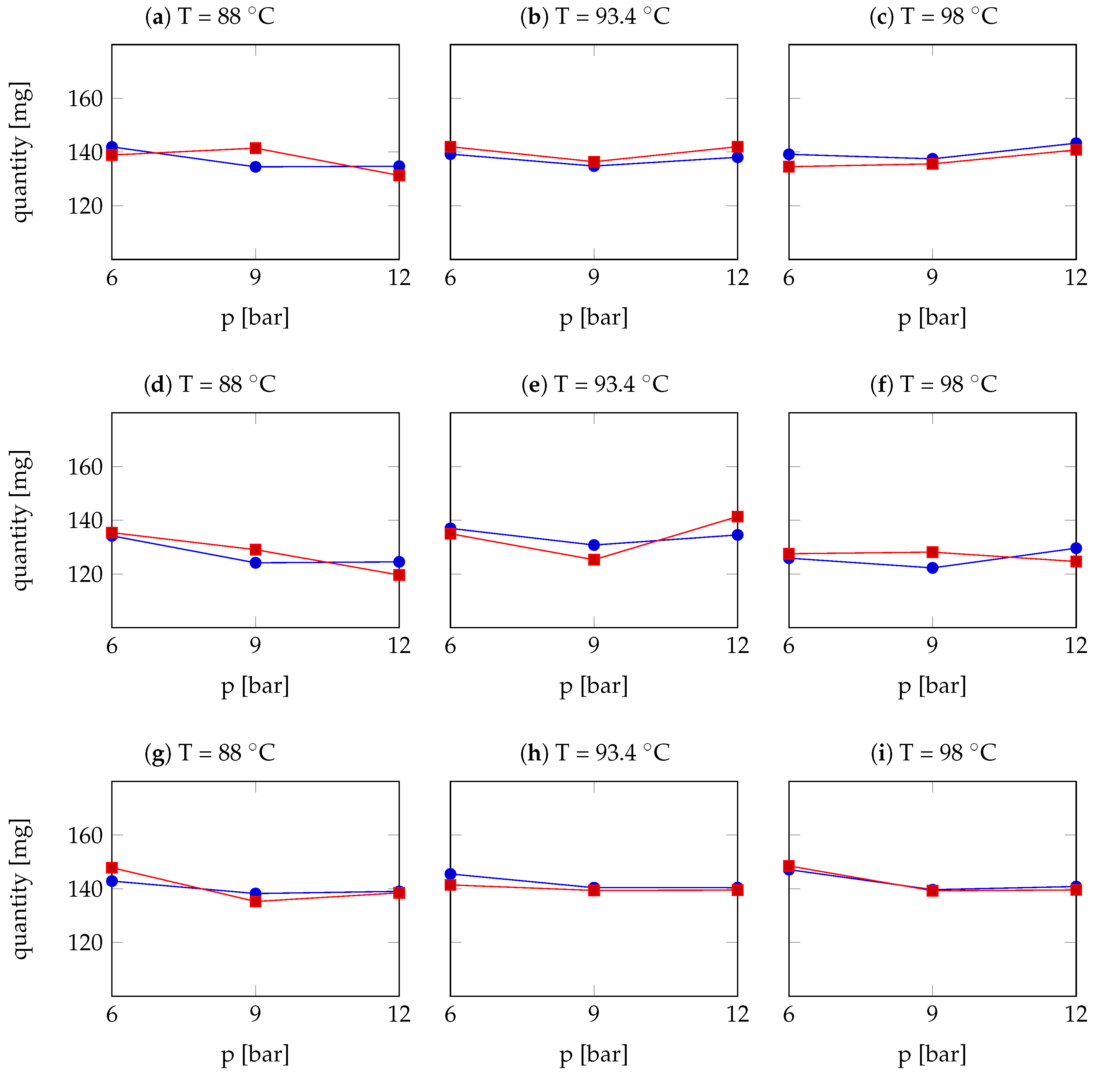
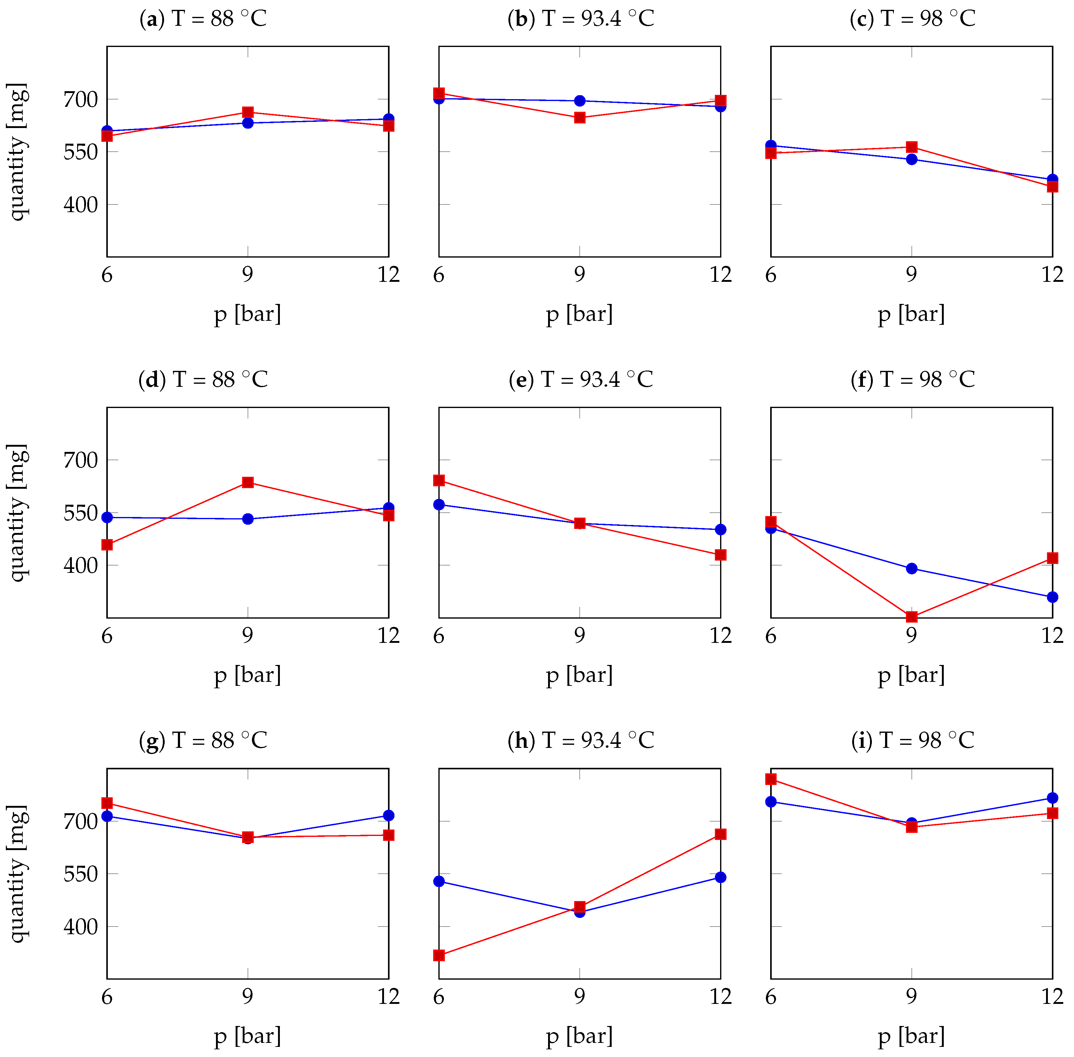
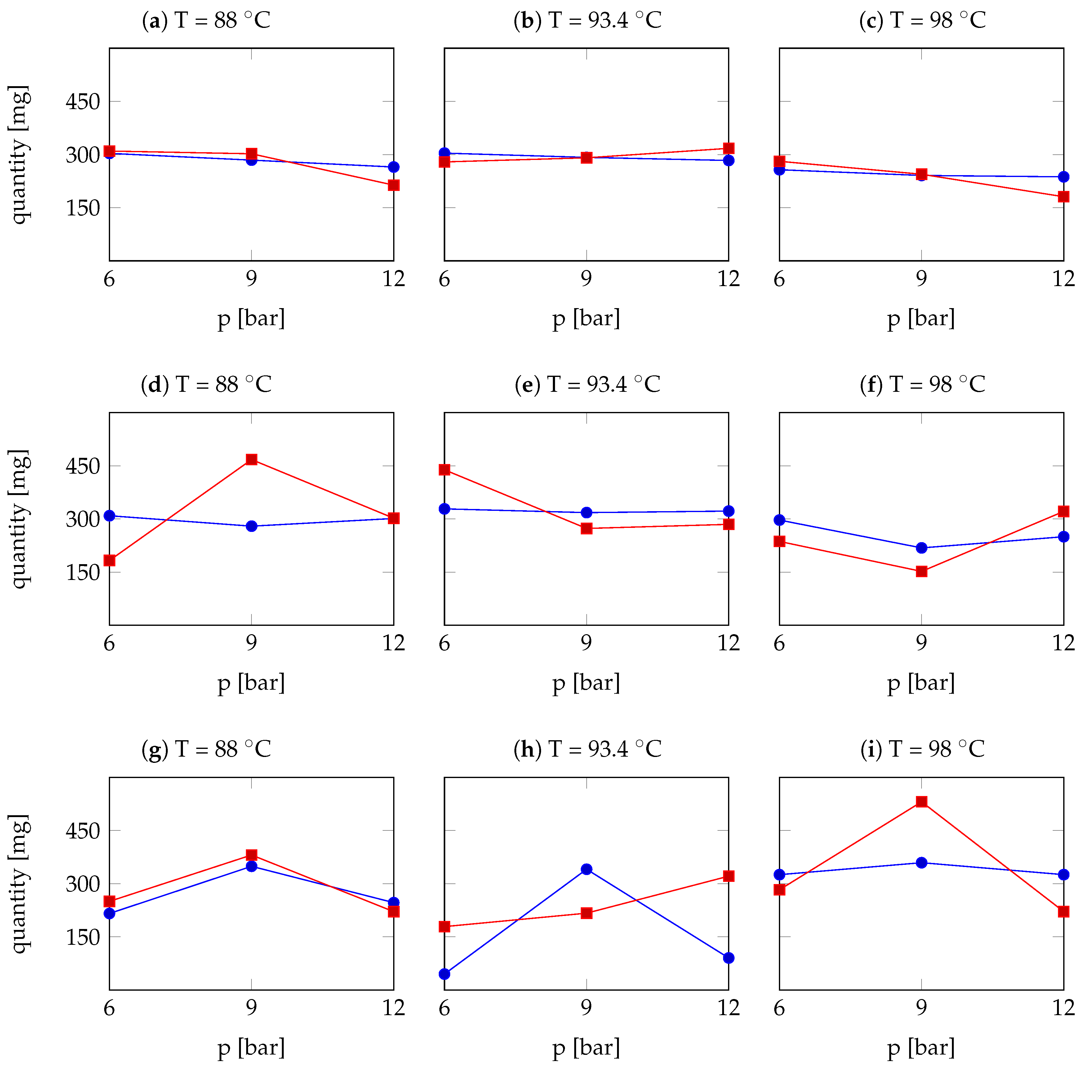
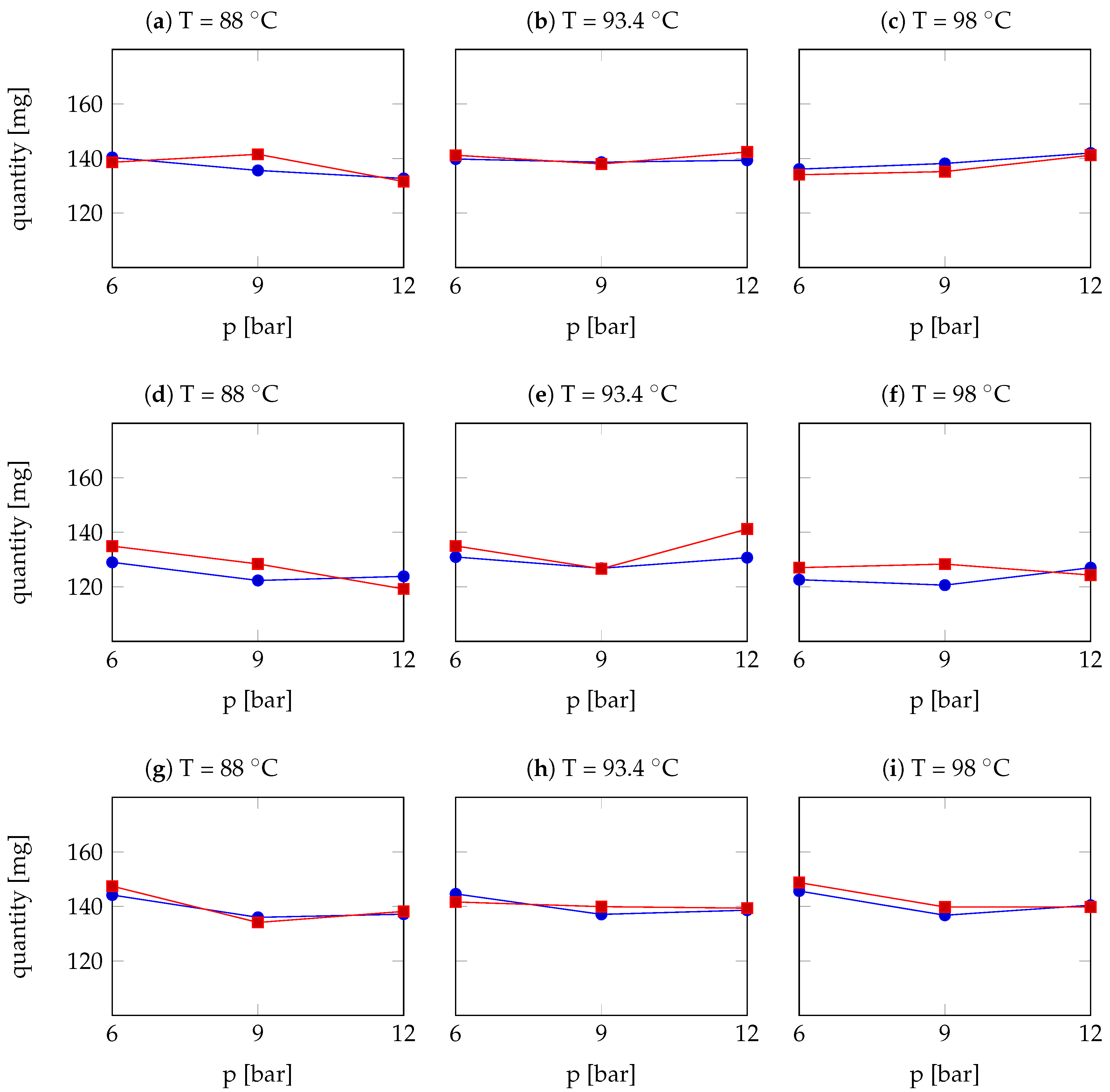
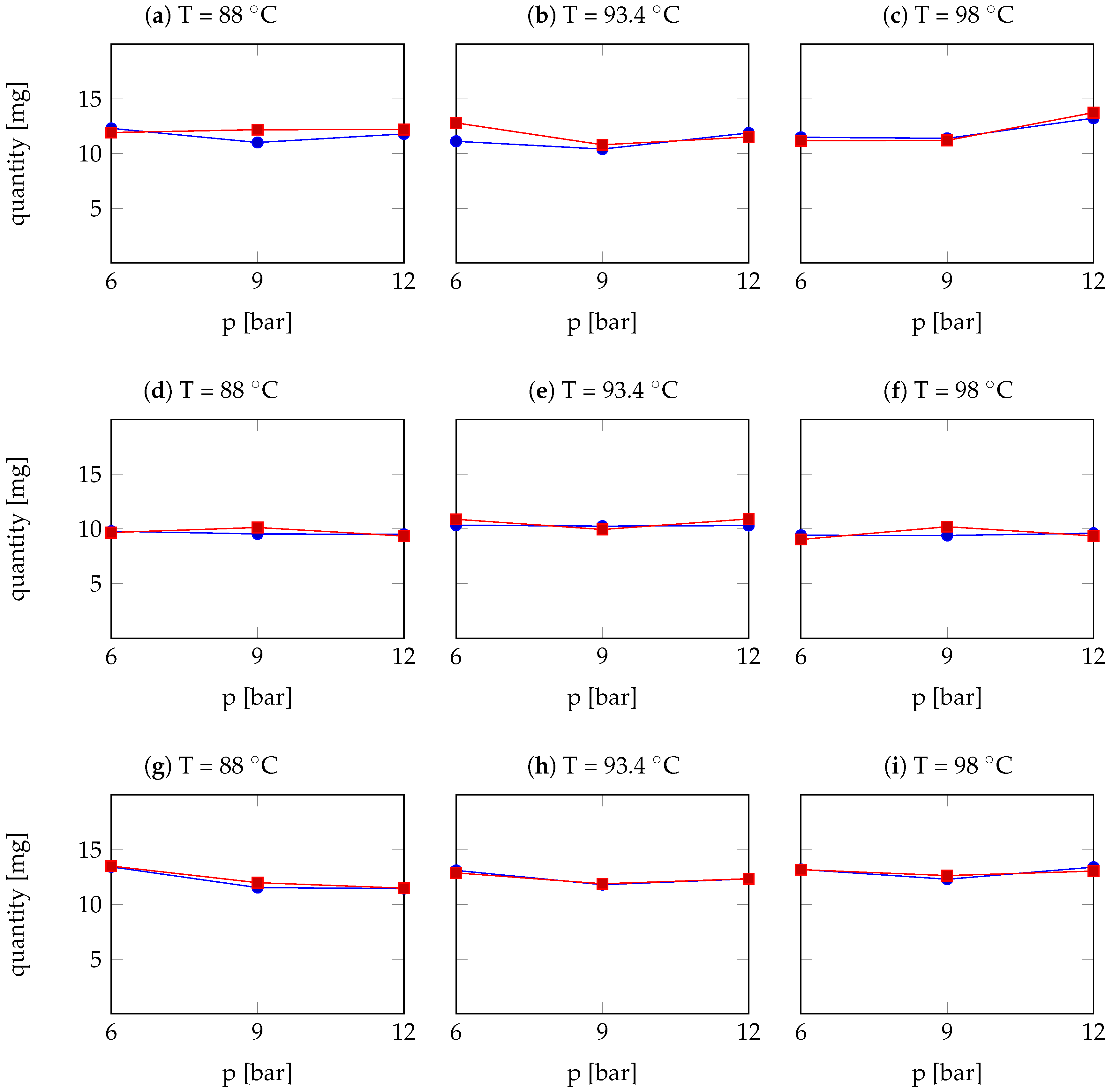
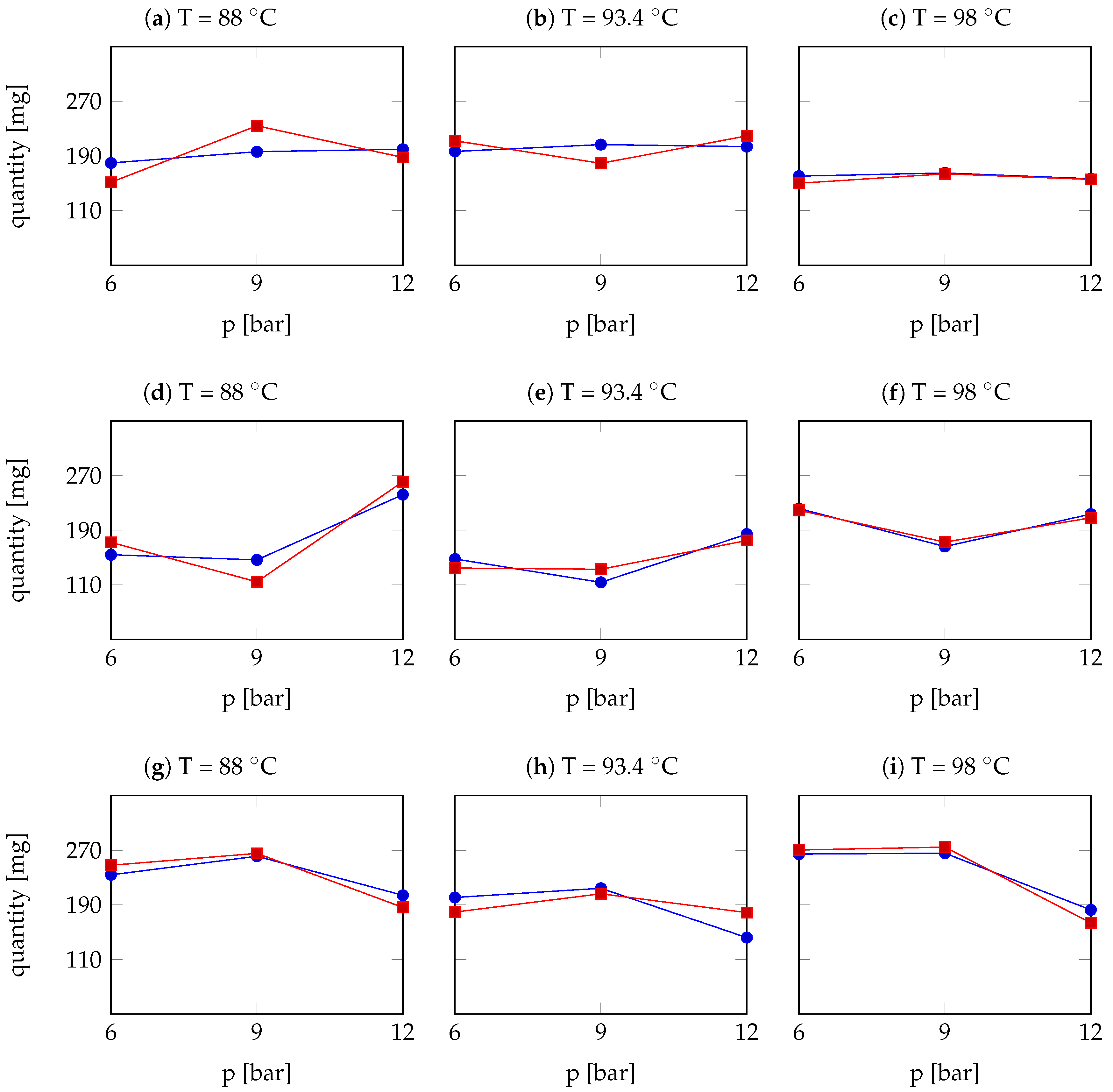
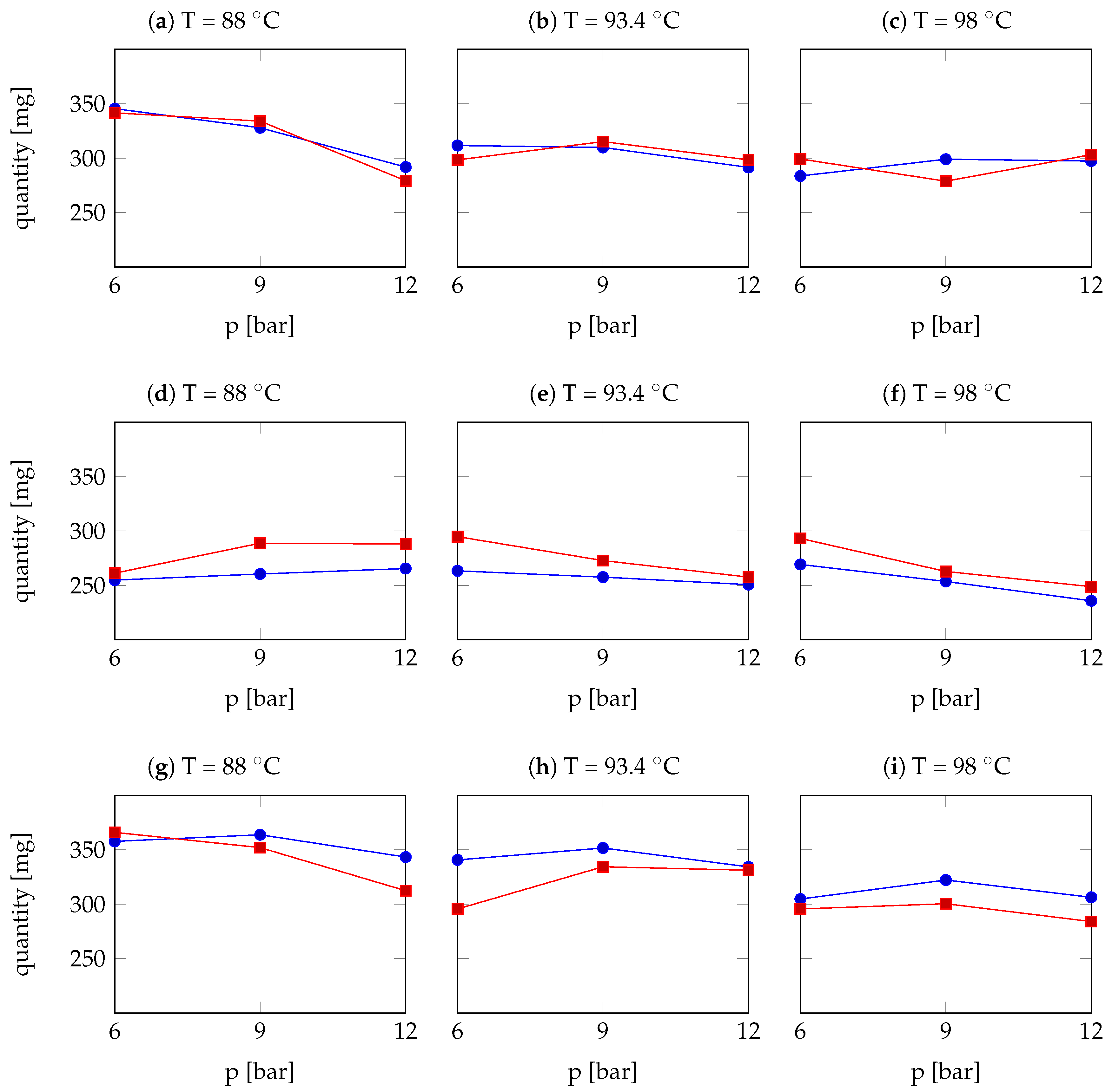
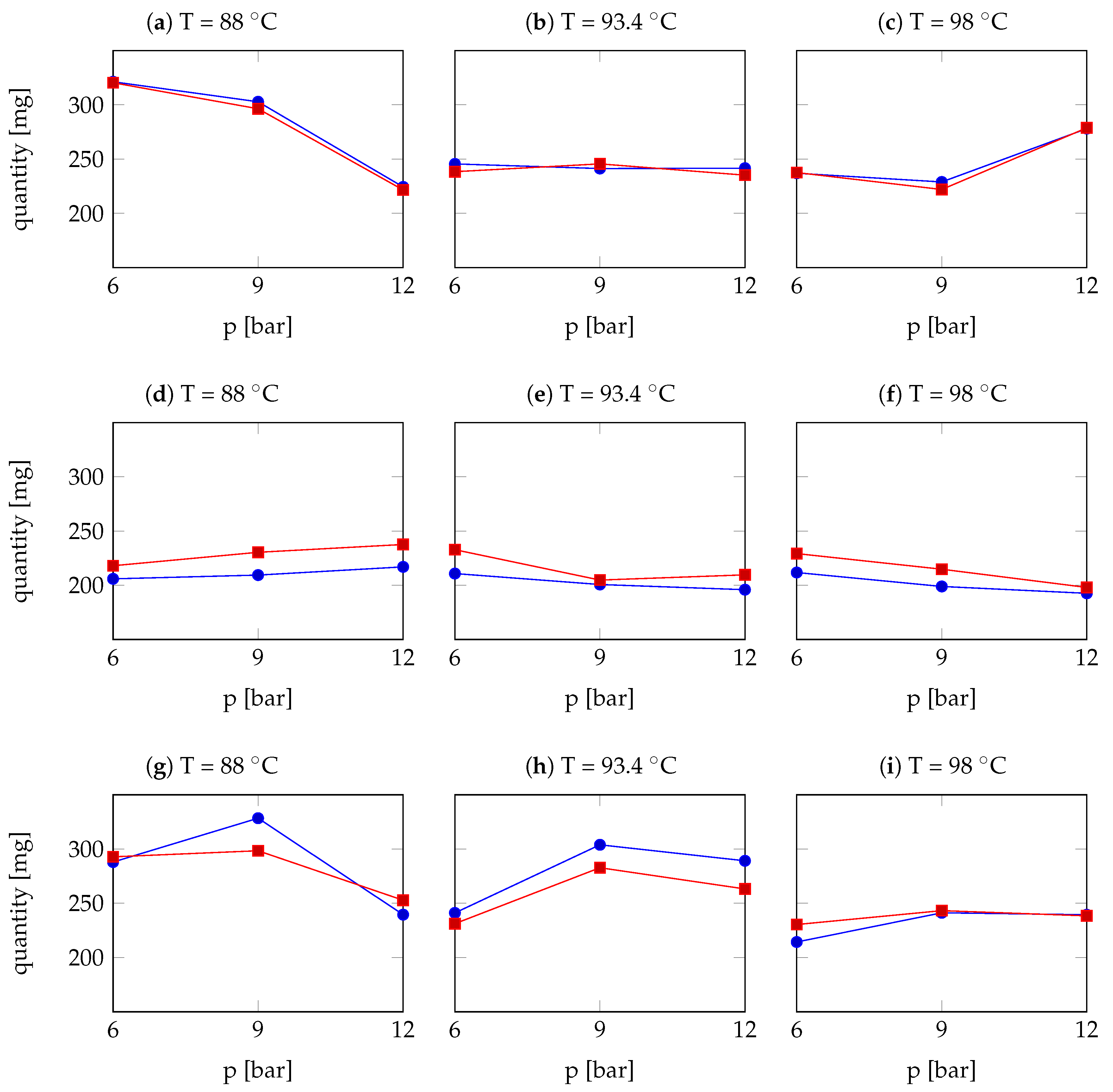
3.2.3. Results: Comparison and Discussion

We first show and discuss the results of the model calibration, then the results of the model validation, giving relevance to the comparison of chemical species between the numerical and laboratory results. Figure 3, Figure 4, Figure 5, Figure 6, Figure 7, Figure 8, Figure 9 and Figure 10 show the extracted amounts of each chemical species in a double cup of about 40 mL, for all the points of the extraction grid used in the calibration, restricting the focus on the Arabica variety. In each figure, the red profiles with square markers display the results from chemical laboratory analyses already described in Section 3.1, see Table 3, Table 4 and Table 5 for details, whereas the blue profiles with circle markers give the results from numerical simulations based on the model (1)–(7). Moreover, in these figures, each row refers to a granulometry—optimal to coarse to fine from top to bottom, each column refers to a temperature and the plots are a function of pressure. The comparison between the red and blue profiles shows a good agreement, especially for the caffeine, chlorogenic acids, trigonelline, tartaric acid and ferulic acid. For the citric acid and the lipids, the correspondence between numerical and analytical results is good, except for some points where peaks occur. In this case, the numerical results give a smooth curve between the maximum and the minimum values of laboratory results. Less correspondence is found for the acetic acid because this species shows a definitely not smooth behaviour of the dissolution coefficient thus the corresponding model of the reactive terms struggles to follow the peaks. However, the general trend of these results is again to smooth the curves of the laboratory results.

Figure 11, Figure 12, Figure 13, Figure 14, Figure 15, Figure 16, Figure 17 and Figure 18 show the extracted amounts of each chemical species in a double cup of about 40 mL for all the points of the extraction grid used in the calibration, restricting the focus on the Robusta variety. These results show similar behaviour to the ones obtained for the Arabica coffee powder, with an overall correspondence between the red and blue profiles slightly decreased, especially for the lipids, but with improved correspondence in the critical species citric acid and acetic acid.

Concerning the amount of in silico liquid coffee, the volumes fall in the interval $[39.4,40.9]$  ${\mathrm{cm}}^3$ for all the cases, which completely agrees with $40\pm 2$${\mathrm{cm}}^3$ of coffee in a double cup, that is what expected from the real extraction. The equivalence between mass and volume is assumed to be valid.

Table 9. Amount (mg) of the chemical species at the end of the percolation process for Arabica variety. The percentage error between numerical and laboratory results is in brackets. The extraction point is denoted by $(T,p,r)$.

	(91, 8, O)	(96, 9, O)	(89, 10, G)	(97, 7, G)	(90, 8, F)	(95, 11, F)
CF	215.2 (7.2)	216.0 (11.4)	186.9 (3.0)	192.0 (7.9)	221.2 (3.5)	213.9 (21.5)
CQA	369.6 (1.9)	351.4 (10.6)	324.8 (6.6)	304.5 (8.0)	347.6 (7.3)	349.5 (22.4)
TR	135.4 (12.2)	136.1 (6.5)	125.8 (5.4)	126.9 (5.7)	140.3 (5.3)	140.2 (27.2)
CA	697.2 (96.1)	634.2 (21.8)	542.2 (17.4)	493.4 (21.1)	523.2 (29.0)	541.4 (3.5)
AA	297.8 (59.6)	275.2 (5.9)	299.0 (42.9)	298.8 (12.5)	336.3 (48.1)	321.4 (72.2)
TA	138.4 (10.0)	138.8 (8.6)	123.8 (6.5)	123.4 (2.5)	138.1 (6.4)	137.6 (24.3)
FA	10.5 (17.2)	10.8 (0.3)	9.8 (9.7)	9.7 (0.2)	12.0 (1.4)	12.3 (30.0)
LP	207.0 (76.0)	188.9 (55.8)	151.9 (6.7)	172.2 (24.6)	232.4 (1.2)	188.5 (0.9)

and

Table 10. Amount (mg) of the chemical species at the end of the percolation process for Robusta variety. The percentage error between numerical and laboratory results is in brackets. The extraction point is denoted by $(T,p,r)$.

	(91, 8, O)	(96, 9, O)	(89, 10, G)	(97, 7, G)	(90, 8, F)	(95, 11, F)
CF	322.5 (0.7)	303.3 (9.6)	261.2 (6.6)	264.0 (9.7)	362.0 (19.4)	336.1 (9.4)
CQA	270.6 (6.4)	228.5 (4.3)	208.4 (7.1)	207.0 (11.5)	318.1 (31.7)	290.4 (20.8)
TR	115.1 (1.8)	109.6 (11.8)	99.8 (2.9)	96.5 (9.7)	136.7 (22.9)	122.7 (20.8)
CA	729.5 (23.4)	763.7 (0.5)	772.4 (18.4)	648.3 (0.7)	844.9 (16.8)	781.6 (8.2)
AA	520.9 (23.1)	465.3 (30.7)	505.1 (7.3)	453.7 (11.0)	503.4 (39.8)	370.3 (5.2)
TA	108.9 (4.8)	104.0 (7.9)	99.7 (2.6)	92.6 (10.9)	131.7 (24.7)	115.3 (15.8)
FA	15.6 (15.2)	15.3 (1.8)	13.2 (5.8)	13.8 (3.9)	21.6 (31.9)	19.8 (23.6)
LP	34.9 (29.1)	34.4 (157)	38.9 (14.6)	30.8 (24.5)	24.9 (30.0)	30.0 (18.0)

show the results of the validation process. In particular, the extraction points are specified along the columns and the chemical species along the rows. In Table 9, for the Arabica variety, apart from the citric acid, the acetic acid and the lipids, which have the worst performance even in the calibration process. The other species have most of the percentage errors (shown in brackets) less than 10% (these values are in bold type), some around 20% and very few greater than 20%. Table 10 shows the corresponding results for the Robusta variety. If we discard the lipids at the point $(96,9,\mathrm{O})$, the percentage errors are slightly higher on average but their dispersion is smaller than in the Arabica variety and very high errors are not reached. To sum up,

Table 11. Mean percentage error among the numerical and laboratory results for each chemical species and Arabica (A) and Robusta (R) varieties.

	CF	CQA	TR	CA	AA	TA	FA	LP
A	9.1	9.4	10.4	31.0	40.2	9.7	9.8	27.5
R	9.2	13.6	11.7	11.3	19.5	11.1	13.7	45.5

gives an overview of the predictability of the model, showing the mean percentage error of each species, averaged over all the validation points.

4. Conclusions

This work describes a fluid dynamics model for water percolation in a porous medium and uses this model to fully characterise the extraction process of EC. The proposed approach relies on reasonable simplifying hypotheses that allow a reliable description of the relevant physico-chemical phenomena characterising the EC percolation process. The resulting model is able to compute the heat transfer, the dynamics of the water and especially the most relevant chemical compounds that constitute a cup of EC. In this paper, the model undergoes a calibration and validation process, based on the following experiment: the comparison of the extracted chemical species between numerical results over in silico EC and laboratory results over real EC. A large extraction campaign has been dedicated to the model calibration. The extraction grid takes into account the variation of water temperature and pressure, granulometry and variety of the coffee powder. A smaller set of extractions in scattered points has been dedicated to the model validation. The comparison shows an extremely good correspondence for some species and a generally good behaviour for all the species, with a mean error in the predictive power around 10% in most cases.

The present study has some limitations that should be analysed in future pre-commercial trials. In particular, the following factors influencing the chemical characteristics of EC have been considered stable or of negligible influence during the extraction campaign. The tamping pressure is fixed at a value that is the mean value when extractions are performed by skilled baristas. Coffee extraction is also influenced by environmental factors, whose variability has been reduced as much as possible in this study since samples have been prepared in a few hours and with macroscopic characteristics of the laboratory fairly constant. The repeatability of the results should be tested against larger variability of the environmental factors, such as ambient temperature, air humidity and water quality. Of course, the extraction equipment also plays a relevant role and a high-quality espresso machine and grinder have been chosen but other equipment available on the market should also be considered. Finally, the whole extraction procedure, involving the proper settings and treatment of the raw material, has been executed by experienced baristas, who significantly limit human error, and this feature is essential to ensure consistency and promise repeatability of the results. In contrast, extraction conditions and granulometry vary in a proper admissible range, and the coffee variety considers pure varieties, discarding blends, for which the chemical characterisation is assumed to follow the linear interpolation of the results of this study.

Future studies can further enhance the predictability of the model by refining some aspects: firstly, the less accurate species such as acetic acid and lipids deserve a deeper investigation on their analyses variability and the modelling of their reaction terms; moreover, an in-depth study on fines would enlarge the applicability area of the model, giving information on the appreciated “crema” of EC and providing the capability to simulate the creation of the compact layer and connected critical situations, such as the clog of the filter.

The good predictive capabilities of the presented model make this simulation system a strategic tool for the coffee market, as it could actually support the current main challenges of the coffee industry, which are the personalisation of the coffee beverage, the sustainability of the coffee chain by reducing the coffee powder used and the research towards innovative extraction techniques.

References

1. Coffee Consumption by Country. Available online: https://wisevoter.com/country-rankings/coffee-consumption-by-country/ (accessed on 30 January 2023).
2. Angeloni, S.; Mustafa, A.M.; Abouelenein, D.; Alessandroni, L.; Acquaticci, L.; Nzekoue, F.K.; Petrelli, R.; Sagratini, G.; Vittori, S.; Torregiani, E.; et al. Characterization of the aroma profile and main key odorants of espresso coffee. Molecules 2021, 26, 3856. [Google Scholar] [CrossRef]
3. Heckman, M.A.; Weil, J.; De Mejia, E.G. Caffeine (1, 3, 7-trimethylxanthine) in foods: A comprehensive review on consumption, functionality, safety, and regulatory matters. J. Food Sci. 2010, 75, R77–R87. [Google Scholar] [CrossRef]
4. Kraehenbuehl, K.; Page-Zoerkler, N.; Mauroux, O.; Gartenmann, K.; Blank, I.; Bel-Rhlid, R. Selective enzymatic hydrolysis of chlorogenic acid lactones in a model system and in a coffee extract. Application to reduction of coffee bitterness. Food Chem. 2017, 218, 9–14. [Google Scholar] [CrossRef]
5. Baeza, G.; Amigo-Benavent, M.; Sarriá, B.; Goya, L.; Mateos, R.; Bravo, L. Green coffee hydroxycinnamic acids but not caffeine protect human HepG2 cells against oxidative stress. Food Res. Int. 2014, 62, 1038–1046. [Google Scholar] [CrossRef] [Green Version]
6. Liang, N.; Kitts, D.D. Role of chlorogenic acids in controlling oxidative and inflammatory stress conditions. Nutrients 2015, 8, 16. [Google Scholar] [CrossRef] [Green Version]
7. Tajik, N.; Tajik, M.; Mack, I.; Enck, P. The potential effects of chlorogenic acid, the main phenolic components in coffee, on health: A comprehensive review of the literature. Eur. J. Nutr. 2017, 56, 2215–2244. [Google Scholar] [CrossRef]
8. Khamitova, G.; Angeloni, S.; Fioretti, L.; Ricciutelli, M.; Sagratini, G.; Torregiani, E.; Vittori, S.; Caprioli, G. The impact of different filter baskets, heights of perforated disc and amount of ground coffee on the extraction of organics acids and the main bioactive compounds in espresso coffee. Food Res. Int. 2020, 133, 109220. [Google Scholar] [CrossRef]
9. Illy, A.; Viani, R. Espresso Coffee: The Science of Quality; Academic Press: Cambridge, MA, USA, 2005. [Google Scholar]
10. Folmer, B. The Craft and Science of Coffee; Academic Press: Cambridge, MA, USA, 2016. [Google Scholar]
11. Moroney, K.M.; Lee, W.T.; O’Brien, S.; Suijver, F.; Marra, J. Asymptotic Analysis of the Dominant Mechanisms in the Coffee Extraction Process. SIAM J. Appl. Math. 2016, 76, 2196–2217. [Google Scholar] [CrossRef] [Green Version]
12. Moroney, K.M.; O’Connell, K.; Meikle-Janney, P.; O’Brien, S.B.G.; Walker, G.M.; Lee, W.T. Analysing extraction uniformity from porous coffee beds using mathematical modelling and computational fluid dynamics approaches. PLoS ONE 2019, 14, e0219906. [Google Scholar] [CrossRef] [Green Version]
13. Cameron, M.I.; Morisco, D.; Hofstetter, D.; Uman, E.; Wilkinson, J.; Kennedy, Z.C.; Fontenot, S.A.; Lee, W.T.; Hendon, C.H.; Foster, J.M. Systematically improving espresso: Insights from mathematical modeling and experiment. Matter 2020, 2, 631–648. [Google Scholar] [CrossRef] [Green Version]
14. Egidi, N.; Giacomini, J.; Maponi, P.; Perticarini, A.; Cognigni, L.; Fioretti, L. An advection–diffusion–reaction model for coffee percolation. Comput. Appl. Math. 2022, 41, 229. [Google Scholar] [CrossRef]
15. Giacomini, J.; Maponi, P.; Perticarini, A. CMMSE: A reduced percolation model for espresso coffee. J. Math. Chem. 2022, 61, 520–538. [Google Scholar] [CrossRef]
16. Moroney, K.; Lee, W.; O’Brien, S.; Suijver, F.; Marra, J. Modelling of coffee extraction during brewing using multiscale methods: An experimentally validated model. Chem. Eng. Sci. 2015, 137, 216–234. [Google Scholar] [CrossRef]
17. Giacomini, J.; Khamitova, G.; Maponi, P.; Vittori, S.; Fioretti, L. Water flow and transport in porous media for in-silico espresso coffee. Int. J. Multiph. Flow 2020, 126, 103252. [Google Scholar] [CrossRef]
18. Kuhn, M.; Lang, S.; Bezold, F.; Minceva, M.; Briesen, H. Time-resolved extraction of caffeine and trigonelline from finely-ground espresso coffee with varying particle sizes and tamping pressures. J. Food Eng. 2017, 206, 37–47. [Google Scholar] [CrossRef]
19. Cordoba, N.; Fernandez-Alduenda, M.; Moreno, F.L.; Ruiz, Y. Coffee extraction: A review of parameters and their influence on the physicochemical characteristics and flavour of coffee brews. Trends Food Sci. Technol. 2020, 96, 45–60. [Google Scholar] [CrossRef]
20. Caprioli, G.; Cortese, M.; Maggi, F.; Minnetti, C.; Odello, L.; Sagratini, G.; Vittori, S. Quantification of caffeine, trigonelline and nicotinic acid in espresso coffee: The influence of espresso machines and coffee cultivars. Int. J. Food Sci. Nutr. 2014, 65, 465–469. [Google Scholar] [CrossRef]
21. Nespresso. Available online: https://www.nespresso.com/it/it/vertuo-system (accessed on 30 January 2023).
22. Bear, J.; Bachmat, Y. Introduction to Modeling of Transport Phenomena in Porous Media; Springer Science & Business Media: Berlin/Heidelberg, Germany, 2012; Volume 4. [Google Scholar]
23. Vafai, K. Handbook of Porous Media; CRC Press: Boca Raton, FL, USA, 2015. [Google Scholar]
24. Egidi, N.; Gioia, E.; Maponi, P.; Spadoni, L. A numerical solution of Richards equation: A simple method adaptable in parallel computing. Int. J. Comput. Math. 2018, 97, 2–17. [Google Scholar] [CrossRef]
25. Diersch, H.J.G. FEFLOW: Finite Element Modeling of Flow, Mass and Heat Transport in Porous and Fractured Media; Springer Science & Business Media: Berlin/Heidelberg, Germany, 2013. [Google Scholar]
26. Mythos 1. Available online: https://www.victoriaarduino.com/mythos-1/ (accessed on 30 January 2023).
27. Puq Press. Available online: https://www.puqpress.com/products/puq-m-line/puqpress-m2-for-mythos/ (accessed on 30 January 2023).
28. VA388 Black Eagle. Available online: https://www.victoriaarduino.com/wp-content/uploads/VA388.pdf (accessed on 30 January 2023).
29. Caprioli, G.; Cortese, M.; Cristalli, G.; Maggi, F.; Odello, L.; Ricciutelli, M.; Sagratini, G.; Sirocchi, V.; Tomassoni, G.; Vittori, S. Optimization of espresso machine parameters through the analysis of coffee odorants by HS-SPME–GC/MS. Food Chem. 2012, 135, 1127–1133. [Google Scholar] [CrossRef]
30. Parenti, A.; Guerrini, L.; Masella, P.; Spinelli, S.; Calamai, L.; Spugnoli, P. Comparison of espresso coffee brewing techniques. J. Food Eng. 2014, 121, 112–117. [Google Scholar] [CrossRef]
31. Efthymiopoulos, I.; Hellier, P.; Ladommatos, N.; Russo-Profili, A.; Eveleigh, A.; Aliev, A.; Kay, A.; Mills-Lamptey, B. Influence of solvent selection and extraction temperature on yield and composition of lipids extracted from spent coffee grounds. Ind. Crop. Prod. 2018, 119, 49–56. [Google Scholar] [CrossRef]
32. Andueza, S.; De Peña, M.P.; Cid, C. Chemical and sensorial characteristics of espresso coffee as affected by grinding and torrefacto roast. J. Agric. Food Chem. 2003, 51, 7034–7039. [Google Scholar] [CrossRef]
33. Severini, C.; Ricci, I.; Marone, M.; Derossi, A.; De Pilli, T. Changes in the aromatic profile of espresso coffee as a function of the grinding grade and extraction time: A study by the electronic nose system. J. Agric. Food Chem. 2015, 63, 2321–2327. [Google Scholar] [CrossRef]
34. Khamitova, G.; Angeloni, S.; Borsetta, G.; Xiao, J.; Maggi, F.; Sagratini, G.; Vittori, S.; Caprioli, G. Optimization of espresso coffee extraction through variation of particle sizes, perforated disk height and filter basket aimed at lowering the amount of ground coffee used. Food Chem. 2020, 314, 126220. [Google Scholar] [CrossRef]
35. Salamanca, C.A.; Fiol, N.; González, C.; Saez, M.; Villaescusa, I. Extraction of espresso coffee by using gradient of temperature. Effect on physicochemical and sensorial characteristics of espresso. Food Chem. 2017, 214, 622–630. [Google Scholar] [CrossRef]
36. Rodrigues, C.I.; Marta, L.; Maia, R.; Miranda, M.; Ribeirinho, M.; Máguas, C. Application of solid-phase extraction to brewed coffee caffeine and organic acid determination by UV/HPLC. J. Food Compos. Anal. 2007, 20, 440–448. [Google Scholar] [CrossRef]
37. Sunarharum, W.B.; Williams, D.J.; Smyth, H.E. Complexity of coffee flavor: A compositional and sensory perspective. Food Res. Int. 2014, 62, 315–325. [Google Scholar] [CrossRef]
38. Severini, C.; Derossi, A.; Ricci, I.; Caporizzi, R.; Fiore, A. Roasting conditions, grinding level and brewing method highly affect the healthy benefits of a coffee cup. Int. J. Clin. Nutr. Diet 2018, 4, 127. [Google Scholar] [CrossRef] [Green Version]
39. Andueza, S.; Maeztu, L.; Pascual, L.; Ibáñez, C.; de Peña, M.P.; Cid, C. Influence of extraction temperature on the final quality of espresso coffee. J. Sci. Food Agric. 2003, 83, 240–248. [Google Scholar] [CrossRef]
40. Campos-Vega, R.; Loarca-Pina, G.; Vergara-Castañeda, H.A.; Oomah, B.D. Spent coffee grounds: A review on current research and future prospects. Trends Food Sci. Technol. 2015, 45, 24–36. [Google Scholar] [CrossRef]
41. FeFlow—DHI. Available online: https://www.mikepoweredbydhi.com/products/feflow (accessed on 30 January 2023).
42. Egidi, N.; Giacomini, J.; Maponi, P. Mathematical model to analyze the flow and heat transfer problem in U-shaped geothermal exchangers. Appl. Math. Model. 2018, 61, 83–106. [Google Scholar] [CrossRef]
43. Giacomini, J.; Invernizzi, M.C.; Maponi, P.; Verdoya, M. Testing a model of flow and heat transfer for u-shaped geothermal exchangers. Adv. Model. Anal. A 2018, 55, 151–157. [Google Scholar]
44. Bear, J.; Verruijt, A. Modeling Groundwater Flow and Pollution; Springer Science & Business Media: Berlin/Heidelberg, Germany, 1987; Volume 2. [Google Scholar]
Figure 1. Domain of the percolation model.
Applsci 13 02688 g001
Figure 2. Particle size distributions of the ground coffee for Arabica variety (a) and Robusta variety (b).
Applsci 13 02688 g002
Figure 3. Comparison between the caffeine extracted through numerical simulations (blue profile with circles) and laboratory measurements (red profile with squares), with different inlet water temperatures and pressures and different grain size of Arabica coffee powder. Figures (ac) show the results of optimal granulometry, Figures (df) of coarse granulometry and Figures (gi) of fine granulometry.
Applsci 13 02688 g003
Figure 4. Comparison between the chlorogenic acids extracted through numerical simulations (blue profile with circles) and laboratory measurements (red profile with squares), with different inlet water temperatures and pressures and different grain size of Arabica coffee powder. Figures (ac) show the results of optimal granulometry, Figures (df) of coarse granulometry and Figures (gi) of fine granulometry.
Applsci 13 02688 g004
Figure 5. Comparison between the trigonelline extracted through numerical simulations (blue profile with circles) and laboratory measurements (red profile with squares), with different inlet water temperatures and pressures and different grain size of Arabica coffee powder. Figures (ac) show the results of optimal granulometry, Figures (df) of coarse granulometry and Figures (gi) of fine granulometry.
Applsci 13 02688 g005
Figure 6. Comparison between the citric acid extracted through numerical simulations (blue profile with circles) and laboratory measurements (red profile with squares), with different inlet water temperatures and pressures and different grain size of Arabica coffee powder. Figures (ac) show the results of optimal granulometry, Figures (df) of coarse granulometry and Figures (gi) of fine granulometry.
Applsci 13 02688 g006
Figure 7. Comparison between the acetic acid extracted through numerical simulations (blue profile with circles) and laboratory measurements (red profile with squares), with different inlet water temperatures and pressures and different grain size of Arabica coffee powder. Figures (ac) show the results of optimal granulometry, Figures (df) of coarse granulometry and Figures (gi) of fine granulometry.
Applsci 13 02688 g007
Figure 8. Comparison between the tartaric acid extracted through numerical simulations (blue profile with circles) and laboratory measurements (red profile with squares), with different inlet water temperatures and pressures and different grain size of Arabica coffee powder. Figures (ac) show the results of optimal granulometry, Figures (df) of coarse granulometry and Figures (gi) of fine granulometry.
Applsci 13 02688 g008
Figure 9. Comparison between the ferulic acid extracted through numerical simulations (blue profile with circles) and laboratory measurements (red profile with squares), with different inlet water temperatures and pressures and different grain size of Arabica coffee powder. Figures (ac) show the results of optimal granulometry, Figures (df) of coarse granulometry and Figures (gi) of fine granulometry.
Applsci 13 02688 g009
Figure 10. Comparison between the lipids extracted through numerical simulations (blue profile with circles) and laboratory measurements (red profile with squares), with different inlet water temperatures and pressures and different grain size of Arabica coffee powder. Figures (ac) show the results of optimal granulometry, Figures (df) of coarse granulometry and Figures (gi) of fine granulometry.
Applsci 13 02688 g010
Figure 11. Comparison between the caffeine extracted through numerical simulations (blue profile with circles) and laboratory measurements (red profile with squares), with different inlet water temperatures and pressures and different grain size of Robusta coffee powder. Figures (ac) show the results of optimal granulometry, Figures (df) of coarse granulometry and Figures (gi) of fine granulometry.
Applsci 13 02688 g011
Figure 12. Comparison between the chlorogenic acids extracted through numerical simulations (blue profile with circles) and laboratory measurements (red profile with squares), with different inlet water temperatures and pressures and different grain size of Robusta coffee powder. Figures (ac) show the results of optimal granulometry, Figures (df) of coarse granulometry and Figures (gi) of fine granulometry.
Applsci 13 02688 g012
Figure 13. Comparison between the trigonelline extracted through numerical simulations (blue profile with circles) and laboratory measurements (red profile with squares), with different inlet water temperatures and pressures and different grain size of Robusta coffee powder. Figures (ac) show the results of optimal granulometry, Figures (df) of coarse granulometry and Figures (gi) of fine granulometry.
Applsci 13 02688 g013
Figure 14. Comparison between the citric acid extracted through numerical simulations (blue profile with circles) and laboratory measurements (red profile with squares), with different inlet water temperatures and pressures and different grain size of Robusta coffee powder. Figures (ac) show the results of optimal granulometry, Figures (df) of coarse granulometry and Figures (gi) of fine granulometry.
Applsci 13 02688 g014
Figure 15. Comparison between the acetic acid extracted through numerical simulations (blue profile with circles) and laboratory measurements (red profile with squares), with different inlet water temperatures and pressures and different grain size of Robusta coffee powder. Figures (ac) show the results of optimal granulometry, Figures (df) of coarse granulometry and Figures (gi) of fine granulometry.
Applsci 13 02688 g015
Figure 16. Comparison between the tartaric acid extracted through numerical simulations (blue profile with circles) and laboratory measurements (red profile with squares), with different inlet water temperatures and pressures and different grain size of Robusta coffee powder. Figures (ac) show the results of optimal granulometry, Figures (df) of coarse granulometry and Figures (gi) of fine granulometry.
Applsci 13 02688 g016
Figure 17. Comparison between the ferulic acid extracted through numerical simulations (blue profile with circles) and laboratory measurements (red profile with squares), with different inlet water temperatures and pressures and different grain size of Robusta coffee powder. Figures (ac) show the results of optimal granulometry, Figures (df) of coarse granulometry and Figures (gi) of fine granulometry.
Applsci 13 02688 g017
Figure 18. Comparison between the lipids extracted through numerical simulations (blue profile with circles) and laboratory measurements (red profile with squares), with different inlet water temperatures and pressures and different grain size of Robusta coffee powder. Figures (ac) show the results of optimal granulometry, Figures (df) of coarse granulometry and Figures (gi) of fine granulometry.
Applsci 13 02688 g018