Abstract
Target localization has been a popular research topic in recent years since it is the basis of all kinds of location-based applications. For GNSS-denied urban or indoor environments, the localization method based on time-of-arrival (TOA) is one of the most popular localization methods due to its high accuracy and simplicity. However, the Non-line-of-sight (NLOS) error is the major cause that degrades the accuracy of the TOA-based localization method. Identifying whether a received signal at a base station (BS) is due to a line-of-sight (LOS) transmission or NLOS is the key to TOA-based localization methods. In the popular LOS signal identification methods, compared with statistic signal methods and machine learning methods, the geometric constraint method has the advantages of simplicity and without requiring priori knowledge of signals and large amounts of training datasets. In this paper, we propose a geometric constraint two-step LOS signal identification method based on common chord intersection point position deviation from mobile stations (MS). In the first step, all BSs are divided into multiple BS combinations with every three BSs, the TOA distance error of each BS combination is estimated based on common chord intersection point position deviation from MS, the BS combinations whose TOA distance error satisfy Gaussian distribution are roughly identified as LOS BS combination and enter the second step, the other BS combinations are discarded as NLOS BS combination. In the second step, based on mutual distance threshold and discrimination result matrix, common chord intersection points of LOS BS combination, and corresponding LOS BS combinations are identified. The BSs of LOS BS combinations are identified as LOS BS and the signals received at LOS BS are identified as LOS signal ultimately. Compared with the other two geometric constraint methods, the proposed algorithm has better identification accuracy, and the setting of the identification threshold value has a theoretical basis, which facilitates the application of the proposed algorithm.
1. Introduction
With the rapid development of the Internet of Things and wireless technology, target localization has been a popular research topic in recent years [1,2,3,4,5,6]. Target localization has a variety of applications, such as emergency assistance, target tracking, geographical routing protocols, environmental monitoring, and intelligent transportation systems. In GNSS-denied urban or indoor environments, accurate localization is still an unsolved problem due to the unavailability or degradation of GNSS signals. For GNSS-denied urban or indoor environments, measurements in localization typically include distance-based parameters such as time-of-arrival (TOA) [7,8,9,10,11] and time-difference-of-arrival (TDOA) [12,13], angle-of-arrival (AOA) [14,15], or their combinations [16]. However, the TOA-based methods, which are also known as range-based methods, are the most common ones due to high accuracy and simplicity.
The TOA-based algorithms have been proved to be very effective when applied to open-air environments, in which the line-of-sight (LOS) paths are dominant. However, Non-line-of-sight (NLOS) radio propagation between source, e.g., mobile station (MS), and sensor, e.g., base station (BS), generally exists in the localization scenarios due to dense obstacles or buildings, which dramatically degrades the performance of TOA-based localization algorithm. NLOS propagation results in time and corresponding distance measurements error. For TOA-based localization algorithm, the extra propagation distance of the NLOS path directly leads to an overestimate of the distance between the source and sensor. This causes a severe degradation of localization accuracy if the TOA-based localization algorithm for LOS scenarios is directly employed. NLOS is considered as the most severe source of TOA-based localization errors [17,18].
To mitigate the NLOS impact, a variety of algorithms have been proposed in the literature. Algorithms for NLOS impact mitigation can be broadly divided into three ways. The first way tries to mitigate the negative impact of NLOS measurements and exploits both LOS and NLOS signals such as propagation model compensation method [19,20,21,22]. This way requires an explicit knowledge of the NLOS propagation model, which has limitations in practical applications. The second way is virtual base station method, which locates the scatterers in NLOS environment firstly, and then regards scatterers as virtual base stations for LOS localization, so the localization of NLOS scenario is converted into a problem of LOS, and its performance depends on the localization accuracy of scatterers [23,24,25,26,27]. This way usually requires assumption or prior knowledge about the scatterer, BS or MS, which limits its applicability in many situations. The third way identifies LOS and NLOS signals first, and then discards NLOS signals, so that only the LOS signals are applied for localization [28,29,30,31,32,33,34,35,36,37,38,39]; unlike the other two ways, it requires at least three LOS signals for localization. The performance of the third way will be close to the Cramer-Rao lower bound (CRLB) when the algorithm has high identification accuracy, therefore, accurately identifying the LOS signals and using them for localization can improve the localization accuracy greatly, we will consider the third way in this paper.
For the identification of LOS/NLOS signals, the algorithms can be mainly divided into three categories. The first category is machine learning method [28,29,30,31], based on training data set and machine learning algorithm, LOS/NLOS signals can be identified. This category of methods requires a large amount of training data for pre-training, and the independent identical distribution (i.i.d) of data cannot be guaranteed usually due to different practical scenarios. The second category is the statistical signal method, which utilizes statistical characteristics of received signal to achieve the identification of LOS/NLOS signals [32,33,34,35]. This category of methods requires priori knowledge of signals, which is an unrealistic assumption in practical scenario usually. The third category is the geometric constraint method, which identifies LOS/NLOS signals based on the spatial geometric relationship between the sensors and source. For the reason of simplicity, only requiring TOA measurements, and without requiring priori knowledge and a large amount of training datasets, the geometric constraint method has received immense attention in the research society [36,37,38,39].
In geometric constraint methods, reference [36] provided residual testing (RT) algorithm, which adopted approximate maximum likelihood (AML) to estimate the position of signal source in recursive procedure based on TOA measurements, if all measurements are LOS signals, then the residuals normalized by the Cramer–Rao lower bound, will have a central Chi-square distribution. If there are NLOS signals, the distribution is noncentral Chi-square. Consequently, LOS/NLOS signals were identified by the residual testing. The authors of [37,38] improved the algorithm of [36] in computational complexity. The authors of [39] provided a two steps area measurement (AM) algorithm. In the initial identification step, the BS combinations including three BSs, whose overlapping area are smaller than threshold or not being, are identified as LOS BS combinations. Then, residual test, overlapping area measurement or statistical method are adopted to identify the LOS signal ultimately. Compared with the RT algorithm, the AM algorithm improves identification accuracy greatly, but the setting of the identification threshold value lacks a theoretical basis, which limits its applicability in practical environments.
In this paper, a novel geometric constraint LOS signal identification method is proposed to improve identification accuracy of LOS signals. Compared with the above two geometric constraint algorithms, the proposed method has better identification accuracy and is more convenient to implement in a practical scenario. The main contributions of this paper are three folds.
1. Better identification accuracy. We propose a two-step LOS signal identification algorithm based on common chord intersection point position deviation from MS. Compared with RT algorithm and AM algorithm, the proposed algorithm has better identification accuracy.
2. Providing the basis of the setting of the identification threshold value. Based on the characteristics of LOS error and Gaussian distribution, we derive the setting of identification threshold value, which facilitates the application of the proposed algorithm. Simulation results are in agreement with the results of derivation.
3. A novel clustering method. Based on characteristic of position distribution of common chord intersection point, we provide a concise and efficient clustering method to identify common chord intersection points of LOS BS combinations.
The remainder of the paper is organized as follows. Section 2 introduces the system model, Section 3 describes the first step of proposed algorithm, and the second step is illustrated in Section 4, Section 5 shows simulation results to demonstrate the effectiveness of the proposed algorithm, and final conclusions are summarized in Section 6.
2. System Model
We consider a two-dimensional (2-D) localization scenario. The task is to locate a source signal, e.g., an MS from the measurements of sensors, e.g., BS, and moreover, MS and BS operate in an environment where NLOS signals may exist. For TOA-based localization algorithm, three BSs are used to locate the MS, the corresponding three BSs are referred to as a BS combination.
The geometric position relationship of three BSs and MS in absence of distance error, including measurement noise error and NLOS error, is depicted as Figure 1. The circle constructed with BS as the center and the distance between the MS and the BS as the radius, is referred to as the localization circle. The connecting line between the intersection points of two localization circles is referred to as the common chord of the two localization circles. Obviously, in environments without measurement noise error and NLOS error, for the same MS and three BSs, the three localization circles intersect at a point, and the corresponding three common chords intersect at a point too. Furthermore, the two intersection points (denoted by point P) all overlap with the position of MS, which is shown in Figure 1.
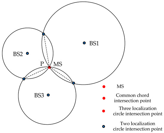
Figure 1.
Demonstration of MS and intersection point (P) in absence of distance error.
However, in practical environments, measurement noise error is inevitable, and NLOS error may occur due to the presence of obstruction. Therefore, the three localization circles no longer intersect at a point although the corresponding three common chords still intersect at a point, and the intersection point of three common chords no longer overlaps with the position of MS, which is depicted as Figure 2.
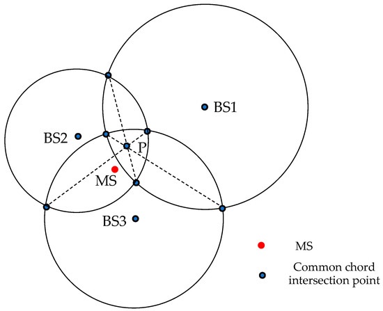
Figure 2.
Demonstration of MS and common chord intersection point (P) in presence of distance error.
For the condition of Figure 2, let is the actual distance between ith BS and MS. The distance error corresponding to , which results from measurement noise error or NLOS error, is denoted as . Then, the measurement of the distance between ith BS and MS, , can be written as
where denotes measurement noise error satisfying Gaussian distribution, and denotes NLOS error with positive value if the ith BS received signal is due to NLOS transmission. Clearly, when the ith BS received signal is due to LOS transmission, , and the corresponding ith BS is referred as LOS BS, otherwise, the ith BS is referred as NLOS BS. So, the identification of LOS/NLOS signals can be converted into the identification of LOS/NLOS BSs.
When the received signals at the three BSs of BS combination are all due to LOS transmission, i.e., , only results from measurement noise error, is small or not being, thus the distance between MS and the intersection point of three common chords (referred as common chord intersection point for simplicity in the following) is small or not being, the BS combination is referred as LOS BS combination. Accordingly, each BS of LOS BS combination is LOS BS, because it only receives LOS signal from MS.
However, if any received signal at the three BSs of BS combination is due to NLOS transmission, i.e., , corresponding is much greater, the distance between MS and common chord intersection point increases greatly, corresponding BS combination is referred to as NLOS BS combination. Among the three BSs of NLOS BS combination, there must be NLOS BS, but the three BSs are not necessarily all NLOS BS.
Therefore, we can identify a BS combination is LOS BS combination or not, based on the distance between MS and common chord intersection point. On the basis of LOS BS combination identification, all BSs of LOS BS combination are identified as LOS BSs
According to this idea, all BSs receiving signal from the same MS are divided into multiple BS combinations with every three BSs, for instance, n BSs can be divided into BS combinations, one BS can belong to multiple BS combinations when the number of BS is more than three. Each BS belonging to LOS BS combination is identified as LOS BS and a BS can be identified as LOS BS because it belongs to any LOS BS combination. The signals received at LOS BSs are identified as LOS signals.
Let the coordinate of the common chord intersection point is , the coordinates of three BSs are and , respectively. Thus, for the case of measurement noise error or NLOS error exist, i.e., , the linear equations of the three common chords can be expressed as Equations (2):
where , . Equations (2) can be rewritten as the form of matrix,
where
Similar to Equation (3), for the case of without measurement noise error and without NLOS error, i.e., , we can obtain
where , and correspond one-to-one to , and for the case of measurement noise error or if the NLOS error exists.
Suppose that coordinate of MS is , and the coordinate deviation of common chord intersection point from MS is , i.e., and , then
where and .
Obviously, is independent of the measurement noise error and NLOS error, but the two categories error all have impact on .
Similarly, dividing the other two variables of Equation (3) into two parts: error-related and error-independent, Equation (3) can be written as
where , , and
Let
which is independent of measurement noise error and NLOS error, and
which is related to measurement noise error and NLOS error.
Substitute (7) into (9), and note that only depends on the coordinates of BSs, which is independent of measurement noise error and NLOS error, i.e., , then we can obtain
3. First Step of Identification Algorithm
For LOS BS combination, there is only measurement noise error, the distance error corresponding to , i.e., , should satisfy Gaussian distribution. Hence, if we can estimate on the basis of measurements of the distance between BS and MS, i.e., , we can identify the LOS BS combination based on whether estimate of satisfies Gaussian distribution. Without loss of generality, suppose that satisfies Gaussian distribution with zero mean and standard deviation when there is only measurement noise error.
If there is only measurement noise error, we can obtain
so, we can approximate as
where
Substitute (15) and (16) into (13) yields
According to Equation (17), if we can obtain the coordinate deviation of common chord intersection point from MS, i.e., , and R, we can obtain an estimate of , i.e., estimate of , and , and then identify LOS BS combination based on whether the estimate of (referred as for simplicity in the following) follows Gaussian distribution, because the estimate of should follow the Gaussian distribution if only measurement noise error exists.
Note R, i.e., , is the actual distance between ith BS and MS, which is unknown. Nevertheless, because of measurement noise error satisfies Gaussian distribution with zero mean, is an unbiased estimate of the measurement of the distance between ith BS and MS, i.e., . Thus, we approximate in R with in (17) for the case of only measurement noise error exists, that is
On the other hand, the coordinate deviation of common chord intersection point from MS, i.e., is unknown, too. Similar to reference [39], for the case of only measurement noise error exists, we can adopt the mean value of the coordinates of three intersection points of three localization circles to approximate the actual coordinate of MS. Meanwhile, the coordinate of common chord intersection point can be solved according to Equation (2). On the basis of approximation of MS coordinate and common chord intersection point coordinate, corresponding coordinate deviation can be solved.
Substitute the approximation of and R into (17), and with least squares method, the estimate of , denoted by , can be obtained as
It should be noted that, though it is cause instead of cause , we can inversely deduce the estimate of according to , and then identify whether the estimate of satisfies Gaussian distribution.
Without loss of generality, we can suppose that . As depicted in Figure 3a, when received signals are all LOS signal, the distance between MS and common chord intersection point is very short, and are all small. However, when the received signal of any BS in BS combination is due to NLOS transmission, i.e., , for instance BS1 in Figure 3b, corresponding NLOS error will result in the distance between MS and common chord intersection point increases greatly, accordingly, increases greatly, too. According to Equation (17), the estimate of will increase greatly, and the estimate of i) will increase greatly, too. Thus, the probability of can be approximated with .
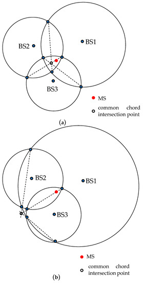
Figure 3.
Demonstration of the variation of distance between MS and common chord intersection point (a) in absence of NLOS error (b) in presence of NLOS error .
For Gaussian distribution, 68.2% of the measurement noise errors lie within 1 standard deviations of the mean and 95.5% lie within 2 standard deviations. Let 1 standard deviations as the identification threshold value of satisfies Gaussian distribution; in other words, if received signals at the three BSs are all due to LOS transmission, they should satisfy the following inequality,
Then, when only measurement noise error exists, the probability of a LOS BS combination is misjudged as a NLOS BS combination, denoted by , is estimated as following
If there are four BSs are LOS BS in all BSs, for any LOS BS of the four LOS BS, it belongs to LOS BS combinations, thus, the probability of this LOS BS is misjudged as NLOS BS is
As shown in Equations (21) and (22), when only measurement noise error exists, for the case of four BSs are LOS BS in all BSs, if we choose one standard deviations as the identification threshold value of only resulting from measurement noise errors, although the probability of a LOS BS combination is misjudged as a NLOS BS combination is up to , the probability of LOS BS is misjudged as NLOS BS is small enough to be neglected. Therefore, we can choose 1 standard deviations as the identification threshold value. As the number of LOS BS continues to increase, the probability of LOS BS is misjudged will decrease dramatically.
Nevertheless, if there are only three BSs are LOS BS in all BSs, for any BS of the three LOS BSs, it only belongs to one BS combination, the probability of LOS BS is misjudged, i.e., the probability of the sole LOS BS combination is misjudged as NLOS BS combination, is up to 31.8%. Therefore, when only measurement noise error exists, for the case of only three BSs are LOS BS in all BSs, identification threshold value of only resulting from measurement noise errors, should be amplified from 1 standard deviations to , corresponding identification inequality is
When only measurement noise error exists, and only three BSs are LOS BS in all BSs, if we choose two standard deviations as identification threshold value of only resulting from measurement noise errors, the probability of LOS BS is misjudged as NLOS BS, which equals to the probability of LOS BS combination is misjudged as NLOS BS combination, is
The probability of LOS BS is misjudged is small enough to be neglected, so we can choose two standard deviations () as the identification threshold value for the case of only three BSs are LOS BS in all BSs. If there are multiple BS combinations satisfying Inequality (23), adopting the same method in [39], the BS combination, which has the least overlapping area, is identified as the sole LOS BS combination. The overlapping area is the area of triangle whose three vertices are intersection points of the three localization circles.
Accordingly, the first step of algorithm procedure can be summarized as follows.
1. All BSs receiving signal from the same MS are divided into multiple BS combinations with every three BSs.
2.1. If there is not any BS combination satisfying inequality (20), the BS combination which satisfy inequality (23) and has the least overlapping area, is identified as LOS BS combination, and the whole identification procedure is completed. If there is not any BS combination satisfying inequality (23), we conclude that the number of LOS BS less than three, and the whole identification procedure is completed.
2.2. If there is only one BS combination satisfying inequality (20), this BS combination is identified as LOS BS combination, and the whole identification procedure is completed.
2.3. If there are more than one BS combination satisfying inequality (20), corresponding BS combinations are roughly identified as LOS BS combination and enter the second step of identification algorithm, the other BS combinations are discarded as NLOS BS combination.
4. Second Step of Identification Algorithm
With identification Inequality (20), LOS BS combinations can be identified roughly. Note that Inequality (20) may have a small probability in presence of NLOS error. Hence, identification Inequality (20) can only roughly identify LOS BS combination, but cannot eliminate all NLOS BS combinations, the remaining will be eliminated by the second step.
For LOS BS combination, the coordinate deviation of common chord intersection point from MS, only results from measurement noise errors. Therefore, corresponding common chord intersection points are randomly distributed near the position of MS, these intersection points are close to each other and are all close to MS. Nevertheless, for the NLOS BS combination, the NLOS error may lead to much greater coordinate deviation between common chord intersection point and MS, which causes corresponding intersection points are far away from that of LOS BS combinations and MS. After the first step, most NLOS BS combination are eliminated, so the intersection points corresponding to the NLOS BS combinations are outliers in all common chord intersection points in the second step. Thus, we can furtherly identify the LOS BS combinations based on the distance between these common chord intersection points.
The schematic diagram of distribution of common chord intersection points after the first step is shown in Figure 4. Most of the common chord intersection points are close to each other and near MS, the other few common chord intersection points, which correspond to NLOS BS combinations, are far away from that of LOS BS combination and MS.
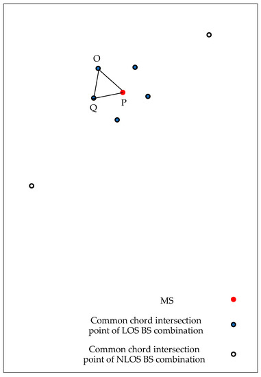
Figure 4.
Geometric position relationship of intersection points of common chords after first step.
To make full use of the characteristic that the common chord intersection points of LOS BS combinations are all near MS and reduce the computational complexity, in this paper, instead of adopting traditional clustering algorithm to identify common chord intersection points corresponding to LOS combination, for every two common chord intersection points, we introduce mutual distance threshold to judge whether the two intersection points are close to each other and whether they are near MS at the same time. For any two intersection points, only the mutual distance is less than the mutual distance threshold, corresponding two intersection points are judged as being close to each other and being near MS. On this basis, for all common chord intersection points in second step, threshold matrix and discrimination result matrix are introduced, then the judgement of whether common chord intersection points are close to each other and whether they are all near MS is achieved.
Now we discuss how to choose the proper mutual distance threshold for judgement of whether two intersection points are close to each other and near MS. The illustration as to how to determine the mutual distance threshold is shown in Figure 4. Point denotes the position of MS, point denotes common chord intersection point of a BS combination, denotes the distance between point and MS. Point and is similar.
Based on (17), we can get
let
(25) would become
According to Equation (27), we can obtain the coordinate deviation of common chord intersection point from MS under the condition of giving ,
where is the element of matrix , and is coordinate deviation of common chord intersection point from MS on X axis and Y axis, respectively.
Taking absolute value in both sides of (28) and (29) and using the inequality relation yields
For the case of LOS BS combination, the distance error of each LOS BS, i.e., only results from measurement noise error. Similar to first step, in Inequality (30) and Inequality (31), in can be approximated by , and let , thus, the upper bound of , denoted by , and upper bound of , denoted by , can be expressed as
Thus, for the ith LOS BS combination, the upper bound of distance between common chord intersection point and MS can be calculated as
where and is upper bound of coordinate deviation between common chord intersection point of ith BS combination and MS on X axis and Y axis, respectively.
As shown in Figure 4, according to the triangle edge-length relation, we can have
Based on Inequality (35), for the case of LOS BS combination, the upper bound of the mutual distance between common chord intersection point of ith BS combination and that of jth BS combination, , can be expressed as
The can be used as the mutual distance threshold to identify whether the two common chord intersection points are close to each other and whether the two common chord intersection points are near MS.
For each pair of BS combinations, there is a corresponding mutual distance threshold. Suppose that there are BS combinations and corresponding common chord intersection points in the second step, the corresponding mutual distance threshold matrix is given by
Let the common chord intersection point distance matrix of BS combinations is
where is the distance between common chord intersection point of ith BS combination and that of jth BS combination.
Subtracting (37) from (38), let , and adopt following discrimination expression
we can obtain the discrimination result matrix
In the discrimination result matrix , the elements of row demonstrate the distance between common chord intersection point of of ith BS combination and that of other BS combinations. illustrates that common chord intersection point of ith BS combination and that of jth BS combination are close to each other and the two intersection points are all near MS. The elements equaling to 1 in row ith form an intersection point set, in which all intersection points are close to each other and near MS. For instance, suppose that in 5th row, , , and equal to 1 and the other elements equal to 0, this denotes that the common chord intersection points of 1st, 2nd, 4th and 5th BS combination are close to each other and are all near MS, and the other intersection points are far away from the above intersection points and MS.
For n rows discrimination result matrix, there are n intersection point sets. In the second step of identification algorithm, most NLOS BS combinations have been eliminated in first step, and the common chord intersection points corresponding to the rest of NLOS BS combinations should be outliers in all intersection points. Therefore, for n intersection point sets of discrimination result matrix, the intersection point set, which has the maximum number of elements equaling to 1, can be identified as the intersection point set corresponds to LOS BS combinations, and the BSs belonging to these LOS BS combinations are identified as LOS BS.
Now, the whole proposed algorithm can be summarized as follows.
1. Construct BS combinations with every three BSs.
2. Calculate the coordinates of three intersection points of three localization circle for each BS combination.
3. Calculate the coordinate of common chord intersection point for each BS combination.
4. Estimate using (19) and then obtain estimate of .
5.1. If there is not any BS combination satisfying (20), identify LOS BS combination with (23), if there is still no BS combination satisfying (23), we conclude that the number of LOS BS less than 3, and the whole identification procedure ends. Otherwise, the BS combination which satisfies (23) and has the least overlapping area, is identified as LOS BS combination, the BSs which belong to this LOS BS combination are identified as LOS BS, and the whole identification procedure ends.
5.2 If there is only one BS combination satisfying (20), it is identified as LOS BS combination, the BSs which belong to this LOS BS combination are identified as LOS BS, and the whole identification procedure ends.
5.3 If there are more than one BS combination satisfying (20), the BS combinations which satisfy (20) are roughly identified as LOS BS combination and enter the second step of identification algorithm, the other BS combinations are discarded as NLOS BS combination.
6. Calculate mutual distance threshold for every two common chord intersection points using (36), then obtain mutual distance threshold matrix with (37).
7. Calculate the distance matrix of all BS combinations.
8. Obtain discrimination result matrix using discrimination expression (39).
9. The intersection point set, which has the maximum number of elements equaling to 1, is identified as common chord intersection point set which corresponds to LOS BS combinations.
10. All BSs belong to LOS BS combination are identified as LOS BS ultimately.
The flow chart of the proposed algorithm is shown in Figure 5.
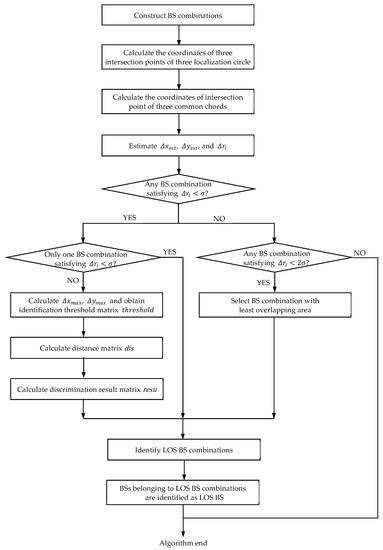
Figure 5.
Flow chart of the proposed algorithm.
5. Simulation and Analysis
Simulations are carried out to evaluate the performance of the proposed algorithm. In order to compare performance of the three geometric constraint algorithms, the same scenario as [36,39] is considered for data generation. As shown in Figure 6, seven BSs are located at (6000, 0), (3000, −6000), (−3000, −5000), (−6000, −1000), (−4000, 6000), (0, 5000) and (4000, 6000), respectively, MS is located at (2000, 1000), all units are in meters. The measurement noise error of distance of TOA satisfies Gaussian distribution with zero mean and standard deviation , equals to 9 or 18, which denotes low measurement noise error or high measurement noise error, respectively. The NLOS error of distance of TOA satisfies uniform distribution from 100 to 1300. Each of the data in the tables below are calculated from 1000 independent trials. In the simulations, the number of LOS BSs varies from three to seven, the NLOS BS and LOS BS are randomly selected from the seven BS for each trial. The correct identification is defined as all LOS BSs are correctly identified and all NLOS BSs are correctly identified, too. The performance of the proposed algorithm is compared with the other two geometric constraint methods, RT algorithm and AM algorithm.
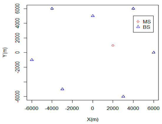
Figure 6.
Geometric position relationship of BSs and MS.
For the case of equals 9, the performance comparison is shown in Table 1. The proposed algorithm outperforms the RT algorithm greatly. Compared with AM algorithm, when there are only three LOS BS, i.e., there is only one LOS BS combination, the two algorithms have the same accuracy because the second step of proposed algorithm cannot be performed, and the two algorithms adopt the same method. However, when there are four or more LOS BS, proposed algorithm outperforms AM algorithm. This demonstrates that the effectiveness of second step of proposed algorithm, which helps to improve the performance of the proposed algorithm when there are more than three LOS BS and at least two BS combinations pass the first step.

Table 1.
Algorithm performance comparation (.
It is observed from Table 2 that when equals to 18, the performance of the proposed algorithm is superior to that of RT algorithm and AM algorithm too. Comparing the results of Table 1 and Table 2, we can see that the performance of all three geometric constraint algorithms degrade with the increasing in standard deviations of measurement noise errors (except for one data of RT algorithm). This is because as increase, the measurement noise error is more easily confused with the NLOS error, which results in the performance degradation of geometric constraint algorithm.
Table 2.
Algorithm performance comparation (.
It can be seen from Table 1 and Table 2, for proposed algorithm, when the number of LOS BSs is four, the probability of BS being misjudged is 1.2% and 5%, respectively. This result approximates the theoretical analysis results of Equation (22). This shows the effectiveness of our theoretical derivation.
6. Conclusions
In GNSS-denied urban or indoor environments, accurate localization is still an unsolved problem due to the unavailability or degradation of GNSS signals. For GNSS-denied urban or indoor environments. TOA-based method is the most common localization method due to high accuracy and simplicity. The localization accuracy could be dramatically degraded if the NLOS signals are misapplied as LOS signals in TOA-based methods. Identifying and localization with the LOS BS can provide performance close to CRLB when the identification algorithm has high identification accuracy and there are at least three LOS BSs. In this paper, a two-step LOS signal identification algorithm exploiting the geometric relationship has been proposed. In the first step, all BSs are divided into multiple BS combinations with every three BSs, the TOA distance error of each BS combination is estimated based on common chord intersection point position deviation from MS, the BS combinations whose TOA distance error estimate satisfy Gaussian distribution are roughly identified as LOS BS combination and enter the second step, the other BS combinations are discarded as NLOS BS combination. In the second step, mutual distance threshold is introduced to judge whether two common chord intersection points are close to each other and whether they are near MS at the same time. On this basis, discrimination result matrix for all common chord intersection points is obtained and then LOS BS combinations are identified. The BSs of LOS BS combinations are identified as LOS BS, and the signals received at LOS BS are identified as LOS signal ultimately. Simulation results show that the proposed algorithm outperforms the other two geometric constraint methods. Simulation results also confirm the effectiveness of our theoretical derivation, which provides a theoretical basis for the setting of the identification threshold value and facilitates the application of proposed algorithm.
Author Contributions
Conceptualization and methodology, R.L. and H.Z.; analysis, R.L. and H.Z.; writing—original draft preparation, R.L. and H.Z.; writing—review and editing, Y.K. and P.D. All authors have read and agreed to the published version of the manuscript.
Funding
This research was funded by National Nature Science Foundation of China [No. 61871332], Sichuan Science and Technology Program [grant numbers: 2021YFG0169], [grant numbers: 2022YFG0190] and Chengdu Normal University Science and Technology Project [no. 111/111159001].
Institutional Review Board Statement
Not applicable.
Informed Consent Statement
Not applicable.
Data Availability Statement
The data used to support the findings of this study are available from the corresponding author upon request.
Acknowledgments
We would like to thank the reviewers for their valuable comments and pointing out possible further research topics.
Conflicts of Interest
The authors declare no conflict of interest.
References
- Tekinay, S.; Chao, E.; Richton, R. Performance benchmarking for wireless location systems. IEEE Commun. Mag. 1998, 36, 72–76. [Google Scholar] [CrossRef]
- Caffery, J.J.; Stuber, G.L. Overview of radiolocation in CDMA cellular systems. IEEE Commun. Mag. 1998, 36, 38–45. [Google Scholar] [CrossRef]
- Drane, C.; Macnaughton, M.; Scott, C. Positioning GSM telephones. IEEE Commun. Mag. 1998, 36, 46–59. [Google Scholar] [CrossRef]
- Luo, J.A.; Zhang, X.P.; Wang, Z.; Lai, X.P. On the accuracy of passive source localization using acoustic sensor array networks. IEEE Sensors J. 2017, 17, 1795–1805. [Google Scholar] [CrossRef]
- Singh, M.; Bhoi, S.K.; Khilar, P.M. Geometric constraint-based range-free localization scheme for wireless sensor networks. IEEE Sensors J. 2017, 17, 5350–5366. [Google Scholar] [CrossRef]
- Wu, Y.I.; Zheng, X. WSN localization using RSS in three dimensional space—A geometric method with closed-form solution. IEEE Sensors J. 2016, 16, 4397–4404. [Google Scholar] [CrossRef]
- Beck, A.; Stoica, P.; Li, J. Exact and approximate solutions of source localization problems. IEEE Trans. Signal Process. 2008, 56, 1770–1778. [Google Scholar] [CrossRef]
- Zou, Y.; Wan, Q. Asynchronous time-of-arrival-based source localization with sensor position uncertainties. IEEE Commun. Lett. 2016, 20, 1860–1863. [Google Scholar] [CrossRef]
- Qiao, T.; Liu, H. An improved method of moments estimator for TOA based localization. IEEE Commun. Lett. 2013, 17, 1321–1324. [Google Scholar] [CrossRef]
- Nguyen, N.-H.; Dogancay, K. Optimal geometry analysis for multistatic TOA localization. IEEE Trans. Signal Process. 2016, 64, 4180–4193. [Google Scholar] [CrossRef]
- Abu-Shaban, Z.; Zhou, X.; Abhayapala, T.D. A Novel TOA-Based Mobile Localization Technique under Mixed LOS/NLOS Conditions for Cellular Networks. IEEE Trans. Veh. Technol. 2016, 65, 8841–8853. [Google Scholar] [CrossRef]
- Zou, Y.; Liu, H.; Xie, W.; Wan, Q. Semidefinite programming methods for alleviating sensor position error in TDOA localization. IEEE Access. 2017, 5, 23111–23120. [Google Scholar] [CrossRef]
- Qiao, T.; Redfield, S.; Abbasi, A.; Su, Z.; Liu, H. Robust coarse position estimation for TDOA localization. IEEE Wirel. Commun. Lett. 2013, 17, 623–626. [Google Scholar] [CrossRef]
- Nguyen, T.L.N.; Shin, Y. A new approach for positioning based on AOA measurements. In Proceedings of the 2013 International Conference on Computing, Management and Telecommunications (ComManTel), Ho Chi Minh City, Vietnam, 21–24 January 2013. [Google Scholar]
- Yin, J.; Wan, Q.; Yang, S.; Ho, K. A simple and accurate TDOA-AOA localization method using two stations. IEEE Signal Process. Lett. 2016, 23, 144–148. [Google Scholar] [CrossRef]
- Pan, T.L.; Chang, J.C.; Shen, C.C. Hybrid TOA/AOA measurements based on the Wiener estimator for cellular network. In Proceedings of the 2015 IEEE 12th International Conference on Networking, Sensing and Control, Taipei, Taiwan, 9–11 April 2015. [Google Scholar]
- Zekavat, S.A.; Buehrer, R.M. Handbook of Position Location: Theory, Practice and Advances, 2nd ed.; Wiley: Hoboken, NJ, USA, 2019. [Google Scholar]
- Wang, L.; Chen, R.; Shen, L.; Qiu, H.; Li, M.; Zhang, P.; Pan, Y. NLOS Mitigation in Sparse Anchor Environments with the Misclosure Check Algorithm. Remote Sens. 2019, 11, 773. [Google Scholar] [CrossRef]
- Li, S.; Hedley, M.; Collings, I.B.; Humphrey, D. TDOA-based localization for semi-static targets in NLOS environments. IEEE Wirel. Commun. Lett. 2015, 4, 513–516. [Google Scholar] [CrossRef]
- Yang, M.; Jackson, D.R.; Chen, J.; Xiong, Z.; Williams, J.T. A TDOA localization method for Nonline-of-Sight scenarios. IEEE Trans. Antennas Propag. 2019, 67, 2666–2676. [Google Scholar] [CrossRef]
- Wu, S.; Zhang, S.; Huang, D. A TOA-based localization algorithm with simultaneous NLOS mitigation and synchronization error elimination. IEEE Sensors. Lett. 2019, 3, 6000504. [Google Scholar] [CrossRef]
- Wang, G.; Zhu, W.; Ansari, N. Robust TDOA-based localization for IoT via joint source position and NLOS error estimation. IEEE Internet Things J. 2019, 6, 8529–8541. [Google Scholar] [CrossRef]
- Zhaounia, M.; Landolsi, M.A.; Bouallegue, R. A novel scattering distance-based mobile positioning algorithm. In Proceedings of the 2009 Global Information Infrastructure Symposium, Hammemet, Tunisia, 22 June 2009. [Google Scholar]
- Yang, T.C.; Jin, L.A. Single station location method in NLOS environment: The circle fitting algorithm. Sci. China-Inf. Sci. 2011, 54, 381–385. [Google Scholar] [CrossRef]
- Liu, D.L.; Liu, K.H.; Ma, Y.T.; Yu, J.X. Joint TOA and DOA localization in indoor environment using virtual stations. IEEE Wirel. Commun. Lett. 2014, 18, 1423–1426. [Google Scholar] [CrossRef]
- Liu, D.L.; Wang, Y.; He, P.; Zhai, Y.; Wang, H.Y. TOA localization for multipath and NLOS environment with virtual stations. EURASIP J. Wirel. Commun. Netw. 2017, 2017, 104. [Google Scholar] [CrossRef]
- Zhang, R.; Xia, W.W.; Yan, F.; Shen, L.F. A single-site positioning method based on TOA and DOA estimation using virtual stations in NLOS environment. China Commun. 2019, 16, 146–159. [Google Scholar]
- Cheng, L.; Wu, X.; Wang, Y. A non-line of sight localization method based on k-means clustering algorithm. In Proceedings of the 2017 7th IEEE International Conference on Electronics Information and Emergency Communication, Macau, China, 21–23 July 2017. [Google Scholar]
- Lyu, W.; Li, Y.; Liu, Z.; Huang, C.; He, R.S. Overview of radiolocation in CDMA cellular systems. In Proceedings of the IEEE International Symposium on Antennas and Propagation and USNC-URSI Radio Science Meeting, Atlanta, GA, USA, 7–12 July 2019. [Google Scholar]
- Beaulieu, N.C.; Young, D.J. Designing time-hopping ultrawide bandwidth receivers for multiuser interference environments. Proc. IEEE 2009, 97, 255–284. [Google Scholar] [CrossRef]
- Maranò, S.; Gifford, W.M.; Wymeersch, H.; Win, M.Z. NLOS identification and mitigation for localization based on UWB experimental data. IEEE J. Sel. Areas Commun. 2010, 28, 1026–1035. [Google Scholar] [CrossRef]
- Benedetto, F.; Giunta, G.; Toscano, A.; Vegni, L. Dynamic LOS/NLOS Statistical Discrimination of Wireless Mobile Channels. In Proceedings of the 2007 IEEE 65th Vehicular Technology Conference, Dublin, Ireland, 22–25 April 2007. [Google Scholar]
- Momtaz, A.; Behnia, F.; Amiri, R.; Marvasti, F. NLOS Identification in Range-Based Source localization: Statistical Approach. IEEE Sensors J. 2018, 18, 3745–3751. [Google Scholar] [CrossRef]
- Yan, L.; Lu, Y.; Zhang, Y. An Improved NLOS Identification and Mitigation Approach for Target Tracking in Wireless Sensor Networks. IEEE Access 2017, 26, 2798–2807. [Google Scholar] [CrossRef]
- Wu, S.X.; Li, J.P.; Liu, S.Y. Single threshold optimization and a novel double threshold scheme for non-line-of-sight identification. Int. J. Commun. Syst. 2015, 27, 2156–2165. [Google Scholar] [CrossRef]
- Chan, Y.T.; Tsui, W.Y.; So, H.C.; Ching, P.C. Time-of-arrival based localization under NLOS conditions. IEEE Trans. Veh. Technol. 2006, 55, 17–24. [Google Scholar] [CrossRef]
- Liu, X.; Wan, Q.; Yang, W.L. Maximum likelihood location for identification of line-of-sight base stations. In Proceedings of the TENCON 2006, 2006 IEEE Region 10 Conference, Hong Kong, China, 14–17 November 2006. [Google Scholar]
- Wann, C.D.; Lin, H.Y. Hybrid TOA/AOA estimation error test and non-line of sight identification in wireless location. Wirel. Commun. Mob. Comput. 2009, 9, 859–873. [Google Scholar] [CrossRef]
- Kuang, L.; Huang, J.Y.; Yang, W.L. Line-of-sight identification based on area measurements. In Proceedings of the International Conference on Automatic Control and Artificial Intelligence, Xiamen, China, 3–5 March 2012. [Google Scholar]


Disclaimer/Publisher’s Note: The statements, opinions and data contained in all publications are solely those of the individual author(s) and contributor(s) and not of MDPI and/or the editor(s). MDPI and/or the editor(s) disclaim responsibility for any injury to people or property resulting from any ideas, methods, instructions or products referred to in the content. |
© 2023 by the authors. Licensee MDPI, Basel, Switzerland. This article is an open access article distributed under the terms and conditions of the Creative Commons Attribution (CC BY) license (https://creativecommons.org/licenses/by/4.0/).