Abstract
With the continuous improvement of people’s living standards, the travel demand for vehicles increases rapidly during weekends and holidays. This situation leads to a number of negative impacts on the transport network, such as traffic congestion, carbon emissions, and long queues at refueling stations. The impact of vehicles requiring energy replenishment on the negative effect is nonlinear. Therefore, the negative effect data of working days cannot be directly used to evaluate the cost, and the traffic equilibrium allocation problem also needs to be solved. An equilibrium allocation model of hybrid vehicles considering the energy replenishment demand in holidays is established, aiming at minimizing the total time cost and energy consumption cost. The Frank–Wolfe algorithm is used to solve the traffic allocation problem in advance, and the negative effect of the urban energy network during holidays is predicted by the Genetic Algorithm—Back Propagation (GA-BP) algorithm. Then, the energy-replenishing vehicles in the traffic network are induced to reduce the total cost. Finally, taking the actual road network in Jiulongpo District of Chongqing City, southwest of China, as an example, the negative effects of multiple stations are predicted. The results show that the prediction method proposed in this paper is effective during holiday periods. In addition, as the market share of electric vehicles increases, the negative cost can decrease gradually. The predicted results can provide a reference for traffic managers.
1. Introduction
The urban transportation energy supply system is one of the most important transportation infrastructure vehicles in the traffic network. At the same time, periodic vehicle energy supplement demand leads to vehicle path deviation, idle queuing and lane change disturbance, resulting in traffic congestion, time delay and other negative effects. This leads to additional negative effects such as carbon emissions and energy consumption, increasing the travel cost of drivers, and intensifying the load of the urban transportation energy supply network, especially during holidays. According to the big data report of 2021 China’s National Day, there are about 2.32 million passengers entering Chongqing City during the holiday, ranking among the top ten tourist cities in China. Electric vehicles may be charged for one hour and queued for four hours. The refueling behavior can lead to additional negative effects such as carbon emissions and other pollutants. However, due to the long charging time and the insufficient number of charging piles, electric vehicles will have negative effects, such as long queuing or detour charging, which may aggravate road congestion.
Analyzing the time-dependent trend of the negative effect can provide a theoretical basis for relieving the refueling load of supply stations and reducing the negative effect of the transportation network. A negative effect prediction system of urban traffic energy supply network is studied aiming at the refueling behavior of heterogeneous vehicles in the traffic network. The prediction system is beneficial to provide management insights for managers and promote the construction of modern energy systems and green intelligent transportation systems. To date, there is little research on urban vehicle energy supplement prediction, and most of the traffic flow prediction focuses on long-term traffic flow prediction and short-term daytime traffic flow prediction. This work presents a method to predict the traffic volume and negative effect cost, especially for the calculation of traffic flow and negative effect cost during holidays.
The remainder of this paper is organized as follows: Section 2 summarizes the relevant research; In Section 3, the composition factors and calculation methods of negative effect cost are analyzed; In Section 4, the prediction model of energy supplement traffic flow in holidays is described; Section 5 includes an modified mixed network equilibrium model; The proposed prediction method and models are verified by using real traffic flow data in Section 6; Finally, the main contributions are concluded and discussed in Section 7.
2. Literature Review
The negative effects of urban transportation energy supply networks during holidays include the negative effects on vehicle driving paths and station operation. To predict the negative effect of vehicle paths, it is necessary to calculate the flow of energy supplement vehicles. However, according to our retrieval of the existing results, no scholars have carried out relevant research on the negative impact of urban transportation energy supply networks during the holiday period. Because of the large difference between the characteristics of travel flow on holidays and weekdays, it is impossible to directly use the weekday travel flow to predict the holiday travel flow. In addition, the use of holiday travel history data alone is limited by factors such as season, temperature, changes in road network structure, and the size of historical data sets, which cannot be accurately predicted. We propose to use the GA-BP algorithm to mine the sequential change of urban traffic trip flow during holidays and calculate the negative impact of the urban traffic energy supply network. Through the traffic allocation model, the flow of energy supplement vehicles under specific demand can be calculated. At present, the research on traffic assignment models at home and abroad is relatively mature, mainly following the principle of user equilibrium Wardorp [1]. The relevant mathematical model of the principle was proposed by Beckmann et al. [2], then, Frank and Wolfe [3] proposed the Frank–Wolfe algorithm to solve the model. Later, the traffic assignment model was divided into a static traffic assignment [4] and dynamic traffic assignment [5,6,7]. Dynamic traffic assignment was based on path selection [8]. For example, Javani et al. [9] proposed a dynamic traffic assignment algorithm based on a fast convergence path. On the basis of route selection, dynamic traffic allocation considering time dimension has been proposed, such as time series [10,11] and daily evolution [12,13]. The negative effects mainly considered in traffic allocation come from environmental pollution [14] and energy consumption [15]; however, the negative effect prediction of urban transportation energy supply network during holidays not only evaluate the distribution of network traffic flow in the time dimension but also consider the negative effects of energy supply stations.
The negative effect on station operation mainly comes from the time delay and carbon emission caused by vehicle queuing [16]. Studies on time delay are mostly about queuing charging delay of electric vehicles [17], while carbon emission models consider mixed vehicle networks frequently. For instance, Cen et al. [18] proposed a Mixed User Equilibrium (MUE) model, which considers the energy supplement behavior of electric vehicles and gasoline vehicles in the urban network. Lucas et al. [19] proposed a method to evaluate energy demands and carbon dioxide emissions from the entire life cycle of electric vehicle and fossil fuel vehicle energy supply sites from construction, maintenance and waste and applied it to a Portuguese case study. It can be seen that although many scholars evaluate the negative effects of vehicle routes and energy replenishment stations, few people integrate the whole transportation energy supply network to study the negative effects of urban transportation energy supply networks during holidays.
Research focusing on traffic forecasting is mainly divided into two aspects one is traffic equilibrium and flow prediction. For example, Ma et al. [20] proposed a new daily traffic flow prediction method and realized it through deep learning, and analyzed the dynamic traffic assignment (DTA) evolution process of the daily traffic flow by combining the relationship between environmental factors and traffic flow. Some scholars also predicted the prediction and correction model of traffic equilibrium after a network interruption accident [21]. For example, Zhou et al. [22] established detailed models of electric vehicle chargers, hydrogen pumps with electrolytes, renewable resources and battery energy storage systems and proposed forecasting methods of renewable energy, electricity price and traffic flow. Station prediction management mostly charges electric vehicles to predict the flow of charging vehicles and the allocation of electric energy resources. However, few scholars consider the flow prediction under time series and the allocation of energy supplement resources of hybrid vehicles.
To sum up, for the prediction of the negative effects of urban transportation energy supply network, most of the existing studies focus on the modeling and analysis of the various parts involved, including the distribution and prediction of traffic network flow and the evaluation and prediction of energy supply stations, but rarely integrate the energy supplement vehicle path and the operation of energy supplement stations to form an urban traffic energy supplement system from the perspective of the whole urban transportation energy supplement system. Therefore, based on the traffic equilibrium assignment model of the urban network, the urban traffic energy supply prediction system is constructed. From the perspective of the negative effect prediction of energy supply stations and energy supply vehicle paths, the hybrid vehicle energy supply problem in daily peak hours and holiday peak hours is considered. The negative effect prediction model of daily energy supply uses the GA-BP learning algorithm. It is difficult to predict the negative effect of energy supplements on holidays, according to daily travel data. The surge of energy supplement demand needs to be solved by using the Frank–Wolfe algorithm by establishing a vehicle equilibrium allocation model to minimize the negative effect of vehicle travel time cost and path energy consumption cost. The feasibility and effectiveness of the model are verified by an actual network example.
3. Measurement of Negative Effects of Energy Supply System
3.1. Measurement of Negative Effects of Energy Supply Stations
The negative effect of urban transportation energy supply stations mainly refers to the negative impact of the station on the surrounding environment during operation, including the energy supplement behavior of vehicles and the operation and construction of the station. The vehicles running on urban roads are divided into electric vehicles and conventional vehicles. Therefore, the transportation energy supply stations can be divided into two categories: the refueling station and the charging station. Refueling stations can quickly fill fossil fuels within five minutes [23]. On the contrary, the charging process needs to take longer time than refueling. The refueling or charging process can cause many negative effects related to influencing factors. The evaluation model can comprehensively consider various factors to analyze the periodic change of negative effects of the station in the time period. Due to the factors involved in the generation of negative effects, an advanced evaluation model should be employed to analyze the changes in the negative effects of stations in a time period.
Combined with the relevant impact research on urban transportation energy supply stations and the negative effect evaluation factors of vehicle energy replenishment behavior, 12 influencing factors are considered as four aspects: traffic efficiency impact, station service impact, environmental impact and safety risk impact. After normalization operations, the weight relationship of 12 influencing factors can be obtained by the entropy weight method, as shown in Table 1.

Table 1.
Weight of each evaluation factor.
Due to the mutual influence and correlation between various index factors, according to the principles of comprehensiveness and measurement convenience, some factors are combined and discarded, and finally, three indexes are selected as representative indexes to measure the negative effects of urban transportation energy supply, namely link driving time, average delay duration and carbon emissions.
Link travel time refers to the time required for vehicles to absolutely pass the link on the front and rear links on the nodes with energy supply stations:
where is the driving time of energy replenishment vehicles on this path link; is the length of the path link before the predicted energy replenishment node; is the average driving speed of vehicles on the path link before the predicted energy replenishment node. Then the cost of path link travel time is:
where is the unit time cost of vehicle driving.
The average delay duration is the mean of the delay time of all replenishment vehicles in unit time, including queuing time and refueling time. According to the M/M/S queuing model, the vehicle replenishment delay time can be obtained:
In Equation (3) is the system service intensity, is the energy supply site j flow to the energy replenishment site per unit of time , the number of independent servers of the site j, and is the service rate per unit of time. Meanwhile, denotes the server idle rate, is the average vehicle waiting time and is the average delay time of vehicles in Equations (4)–(6).
Then the total delay cost can be defined as:
Carbon emissions generate by energy refueling vehicles when they run in the station or idle frequently due to queuing, which is also called cold emission. The emission cost can be expressed as follows:
where is the unit cost of carbon equivalent emissions, is the fuel consumption of the vehicle per hour idle speed, and is the carbon price.
According to the weight relation among the three indicators and normalized treatment, the negative effect coefficient of the site j is calculated as follows:
By measuring the index data of different stations in each time period, we can get the change value of the negative effect coefficient of all stations in the region with time as the original data sample. A cycle is divided into multiple time periods according to the changing relationship of negative effects. The changing trend of the negative effect of stations in the region can be predicted by using a neural network algorithm.
3.2. Measurement of Negative Path Effect of Energy-Supplementing Vehicles
The negative effects of vehicle energy replenishment mainly include vehicle energy consumption, delay time and driver psychological anxiety. The additional driving mileage is converted into the total driving mileage of the driver, and the driving cost of the driver is calculated together with the energy consumption to quantify the negative effect of the driver’s path. Therefore, urban paths are considered as a large transportation network , in which N, A and S are the sets of nodes, links, and energy supply stations, respectively. Any entrance to any exit of the network is set as a starting and ending point (OD). After vehicles with energy supplement requirements enter this area, they are divided into the power supplement stations supported by the vehicles according to their remaining mileage and driving direction. In the network, for all OD pairs of daily travel vehicles, the traffic flow on the path is mainly composed of three types of vehicles, namely, vehicles requiring no energy supplement, electric vehicles requiring energy supplement and fuel vehicles requiring energy supplement. The path that the vehicle passes between the starting and ending pairs is , and the vehicle returns to its OD path after generating the energy supplement demand and completing the energy supplement; when there are no alternative stations on the OD path of the vehicle, path deviation will occur, and extra mileage will be generated; then the new driving path of the vehicle will be updated, where and the path length is . Therefore, the extra mileage generated by path deviation is , where , means that the vehicle is supported and located on the original OD path of the vehicle after generating energy supplement demand.
Assuming that vehicles recharge at most once during travel and that the recharge demand of different types of vehicles is related to their flow, the ratio between electric vehicles and fuel vehicles is set as r, where the charging ratio of electric vehicles is related to the remaining mileage of vehicles and the psychological anxiety degree of drivers is set as , and the formula is:
where is the weighted average travel distance of electric vehicles between OD pairs, and the charging distance of daily travel vehicles should be less than the remaining mileage of vehicles.
According to the change of negative effect in different time periods of energy supply stations on the path , each time period will be allocated iteratively based on the previous time period. If the vehicles that need energy replenishment in the previous time period fail to arrive at the station for energy replenishment after the end of the time period, they will be allocated together with the vehicles that need energy replenishment in the next time period . The link flow of each time period can be obtained, and the negative effect of the vehicle driving path can be calculated. The mileage energy consumption needs to be calculated separately according to different vehicle types. According to the Bureau of Public Road (BPR) function Equations (12) and (13), the link is composed of links , and the length of each link is often different in the actual network, and the traffic capacity is also different according to different link level:
where is the travel time within a time range and is the free outflow travel time of the link in the time period .
where is the segment capacity in the time period , is the free outflow cost of the link in the time period .
4. The Model of Negative Effect Prediction
GA-BP neural network algorithm uses a genetic algorithm to obtain the optimal structural parameters of the BP neural network, and then carries out the training of the neural network, and selects the test set for testing. The algorithm flow is shown in Figure 1.
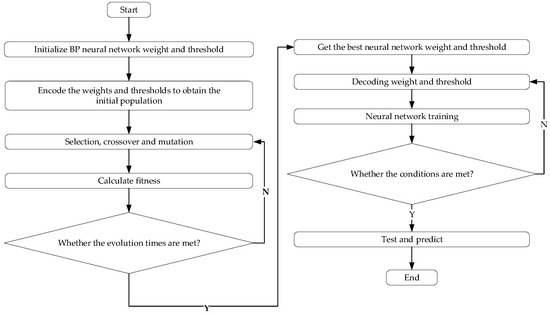
Figure 1.
GA-BP neural network process.
A neural network is the core of a feedforward neural network. It simulates the information transmission mode of biological neurons and realizes machine learning. However, it also has some defects, such as the slow learning convergence speed in the algorithm. In addition, due to its initial weight and threshold, it cannot guarantee to converge to the global optimum. The GA can imitate the natural selection and genetic mechanism of biology and constantly screen and adjust the weight and threshold of the neural network to avoid falling into local optimization.
Three layers of classical networks are used here, namely the input layer, hidden layer and output layer. The output of the transfer function using the Tansig function is any number in range (−1, 1). According to the error comparison of different hidden layers, five hidden layer nodes with the smallest error are selected, and the gradient descent method is used to train under the same error target of 0.00001. Input 365 data sets, the first 292 as the training set and the last 73 as the test set. This group is the negative effect cost data of a single node in a single time period. The GA is the process of selecting the best initial weight and threshold. The relevant parameters are shown in Table 2. This method is suitable for network prediction with complex internal mechanisms and can provide help for the prediction of negative effects of urban transportation energy supply networks.

Table 2.
Ga-BP-related parameters.
Before the forecast, it is necessary to collect the original data of urban transportation energy supply stations in the peak area of the working day and then obtain the forecast value for the next day through the forecast. At the same time, it is also possible to observe the overall trend of traffic flow so as to calculate the negative effect cost. According to the trend characteristics of traffic flow, it can be inferred that the trend of negative effect should be consistent with the traffic flow, and the periodic traffic flow will show obvious time series periodic characteristics. The final prediction result can be obtained by the GA-BP algorithm (see Table 3).

Table 3.
Error comparison of node number in different hidden layers.
5. The Model of Traffic Allocation
The prediction model can predict the negative effect cost of the energy supply network in the daily traffic network. However, due to the surge in the demand of vehicle energy supplement users during holidays, it is impossible to predict directly according to the daily travel flow; consequently, the network traffic flow under special demand can be obtained through the network traffic allocation model. To facilitate calculation and modeling, the time range T is divided into a group of discrete time periods to deal with the negative effects of periodic energy supplements. Different energy supplement stations are located in different locations, so they have different negative effects. In the actual environment, the change of negative effect changes with the flow of energy supplement vehicles, and the flow of energy supplement vehicles is not a continuous and smooth function. According to the changing trend of the unit time, the negative effect of each time period is the cumulative mean value of the negative effect of that period.
5.1. Model Description
In this model, the vehicles with fuel demand in the current time period are allocated based on time series, and the allocation method is based on the path selection with the minimum negative effect. Therefore, the negative effect cost of each part is taken as the edge weight. When the weights are the same, the alternative paths with the same weight are allocated based on the shortest path principle. Assuming that the side weight of the path link is the sum of the weight of the path link and the weight of the energy supply station within the time period , where the path link is located before the station , that is, the energy replenishment vehicle passes through the first path link and arrives at the station , then the side weight of the path link is:
where is the weight coefficient, and F is the energy consumption cost per unit link length; is the binary variable, where is 1 indicates that there is an energy supply site, and 0 indicates that there is no energy supply site available.
The symbols and descriptions of this model are shown in Table 4:

Table 4.
Notations used in the proposed model.
5.2. Equilibrium Model of Mixed Network
In order to obtain the flow on the urban traffic network under the condition of special demand flow during holidays, an improved mixed network equilibrium model [18] is adopted, which is a dynamic vehicle replenishment allocation solution model based on time series. The objective function is defined as follows:
The objective function (15) is the sum of the cumulative travel time cost and the energy consumption cost of the travel path on all links. Equations (16)–(19) are flow conservation constraints between OD pairs. Constraints (21)–(24) means the relationship between path flow and link flow. Constraints (20), (25) and (26) are quantitative relationship constraints. Constraints (27) are a nonnegative constraint on path traffic. Constraints (28) are binary decision variables. The model can be solved by the Frank–Wolfe algorithm, and the link flow allocation results based on time series are obtained, simultaneously.
6. Case Study
To verify the effectiveness of the proposed model and algorithm, the network of Jiulongpo district in Chongqing was taken as an example for checking calculation, as shown in Figure 2. The network consists of 15 nodes and 20 links. There are two refueling and gas station nodes and two charging station nodes in the node. Nodes 6 and 11 represent charging station nodes, and nodes 7 and 10 represent refueling and gas station nodes. Nodes 1 and 4 are the starting points, nodes 2, and 3 are the ending points. Therefore, OD pairs can be represented as 1→2, 1→3, 4→2, and 4→3. There are significant differences in the capacity and flow of different links, which will inevitably have an important impact on the choice of vehicle route. Path-link are divided into three grades, and different grades are represented by arrows of different thicknesses. Path-link 1, 2, 5, 6, 7, 10, 12, 13, 14, and 19 are the first level; path-link 3, 9, 11, 12, 15, 17, 18, and 20 are the second level, and path-link 4 and 8 are the third level.
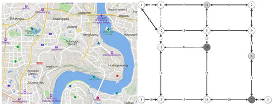
Figure 2.
The real map and the corresponding simplified network.
According to the link level location of each node, the peak data on the actual corresponding grade road is selected for calculation. Figure 3 shows the negative effect changes of four stations from Monday to Thursday from 6:00 a.m. to 12:00 a.m. It can be seen that the negative effect cost reaches a high peak in the morning peak period of nodes 6 and 10. In addition, the peak hour of node 11 is not obvious, showing a high level of negative for a long time, and the time points at which the four nodes lead to the highest peak are different. In addition, it can be observed that node 7 encounters the peak in a short time, while node 6 is on the contrary. Node 6 has a transition time before the peak and drops rapidly after the peak, and node 10 has a transition time before and after the peak hour.
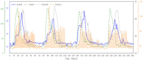
Figure 3.
Change of negative effect in the morning of four days at each node.
To predict the trend of negative effect cost on Friday, it can be obtained by GA-BP algorithm based on the data of the previous four days. The data is measured with five minutes interval. Each station contains 365 data. The front 292 data are used as the training set and the others are used as the test set. The results obtained by the GA-BP algorithm are shown in Figure 4. The prediction error and determination coefficient R2 are shown in Table 5. The average relative error is almost below 0.1 and the R2 coefficient is above 0.98. The average relative percentage error is shown in Figure 5. The average relative percentage error of node 6 is 0.50%, the average relative percentage error of node 7 is 10.70%, the average relative percentage error of node 10 is 3.42%, and the average relative percentage error of node 11 is 2.00%. In addition, the linear regression fitting r value of each part of the neural network result is shown in Figure 6, which shows that the fitting result is good.
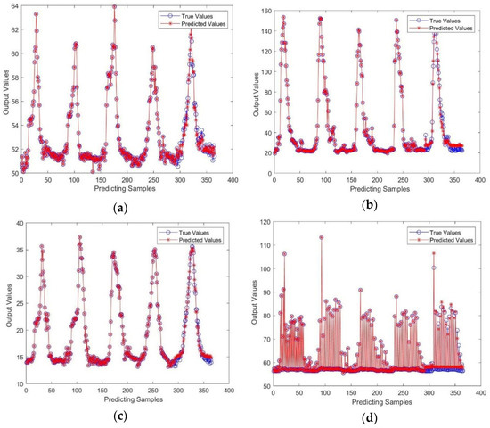
Figure 4.
Predicted and real GA-BP of negative effect at each node. (a) Predicted and true values of node 6. (b) Predicted and true values of node 7. (c) Predicted and true values of node 10. (d) Predicted and true values of node 11.

Table 5.
Prediction errors and determination coefficients of each node.
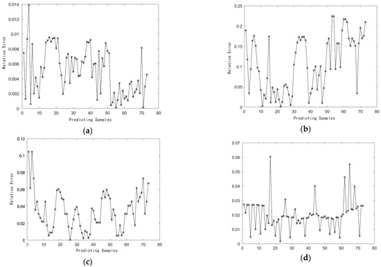
Figure 5.
Comparison of error between GA-BP predicted value and real value of negative effect at each node. (a) Average relative percentage error of node 6. (b) Average relative percentage error of node 7. (c) Average relative percentage error of node 10. (d) Average relative percentage error of node 11.
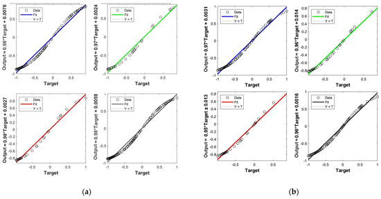
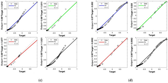
Figure 6.
Regression fitting of GA-BP prediction results in a negative effect at each node. (a) Linear regression fitting of results of Node 6. (b) Linear regression fitting of results of node 7. (c) Linear regression fitting of results of Node 6. (d) Linear regression fitting of results of node 7.
After the prediction results of stations are obtained, the negative effect trend of urban transportation energy supply stations can be observed. The result also shows the changing trend of energy supplement traffic flow with time. Figure 7 shows the predicted negative effects of the four transportation energy supply stations. The negative effects of the four nodes predicted on this day are divided into six time periods according to their incremental trend. It can be seen that the negative effects of the four stations almost begin to rise at the t2 time, and the rising speed and magnitude of node 7 are significantly greater than those of the other three nodes, but the negative effects of node 7 decline rapidly from the t3 time, while node 6 and node 10 are still in the rising stage and the range is not large. Node 11 is in the stage of high negative effects for a long time. In addition, it can be clearly observed that the negative effect of node 11 is slightly greater than that of node 6, much greater than that of node 7 and node 10, and the negative effect of node 10 is at the minimum position.
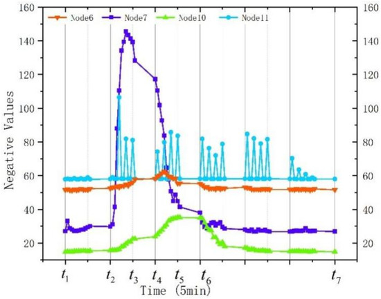
Figure 7.
Temporal relationship between negative effects of different transportation energy supply stations in different stages.
To predict the negative effects of holidays, it is not possible to directly predict the negative effects based on the traffic flow of the previous days. An important reason is that in addition to the daily surrounding travel vehicles, there are additional travel vehicles in the region during holidays. In order to predict the negative effect of energy supplement on holidays, the energy supplement flow in each time period can be obtained through the allocation model according to the divided time period. After the energy supplement flow is obtained, the cost of the negative effect of the energy supplement in this time period can be calculated. Table 6 shows the total demand of each OD for this time period, which is based on the data from last Saturday. At present, the market share of electric vehicles and fuel vehicles in Chongqing is 1:9. The safe driving range of electric vehicles is 170 km, and the anxiety coefficient of power exhaustion is 0.8 [18]. The calculation of side weight mainly includes the weight of path-link and the weight of connected nodes. The BPR function of travel time value adopts classical parameters, and the power cost and fuel cost per unit link length are 0.15 ¥/km and 1.5 ¥/km, respectively [24]. The length of each link of the network is shown in Table 7. The unit time value of the bullet train driver is 3.13 ¥/min.

Table 6.
Total demand in the corresponding time period.

Table 7.
Length of each link of a network.
The traffic flow results obtained by using the flow assignment algorithm are shown in Figure 8. It can be seen that the traffic flow of each link is almost the highest in the time period of 7:10–7:45, followed by 7:45–7:55. In addition, links 9 and 12 are maintained in the low traffic flow range. According to the flow and energy supplement of the four stations, the energy supplement flow of the four nodes in six time periods is summarized and compared, as shown in Figure 9a. From the perspective of the time dimension, the number of energy-replenishing vehicles is the largest in the same period of 7:10–7:45, while there are fewer vehicles in the earliest and noon periods. The comparison trend with the overall driving traffic flow is roughly the same, and the traffic at node 6 is the smallest, and the volume of node 7 is similar to that of node 10, which is determined by the vehicle flow of energy supplement demand. At present, the market share of fuel vehicles still accounts for the absolute counterpart. The same is true for the charging station. Node 11 has a higher flow than node 6. Node 6 is located on the expressway and in the Yangjiaping business district; accordingly, the flow is greater. The reason why node 7 has more traffic than node 10 is determined by the link level and the distance from the end point [25]. In addition, with the gradual increase of electric vehicle market penetration, the proportion of charging demand and energy-replenishing vehicles in the subsequent network will gradually increase. Therefore, the station traffic with different energy-replenishing vehicle types and interest rates is compared. As shown in Figure 9b–d, the traffic to the charging station node is basically the same when the market share is 30%. When the market share is 50%, the traffic flow at the charging station node begins to exceed that at the gas filling station node and completely exceeds that at 80%, even greater than the current gap between the two types of traffic flow.
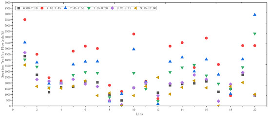
Figure 8.
Results of balanced distribution of traffic flow in different time periods of each path link.
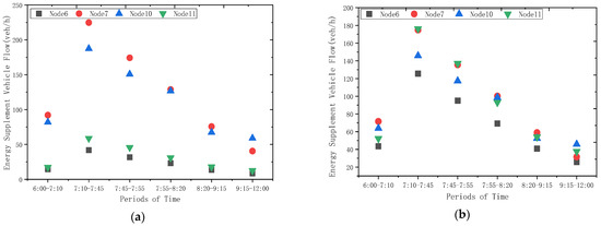
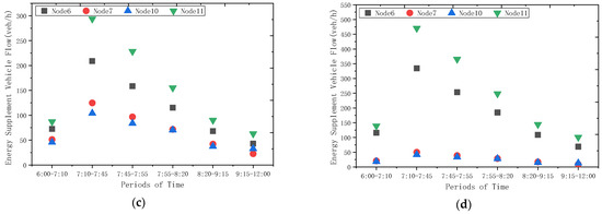
Figure 9.
Equalization distribution results of energy replenished vehicle flow in each time period. (a) 10% of the electric vehicle market. (b) 30% of the electric vehicle market. (c) 50% of the electric vehicle market. (d) 80% of the electric vehicle market.
After obtaining the flow of energy replenishing vehicles, the negative effect cost of each energy replenishing station and the corresponding path can be calculated, as shown in Figure 10a. The cost of the negative effect becomes higher in the two time periods of 7:45–7:55 and 7:55–8:20. The total negative effect cost in the total measurement time is 16,821.52 ¥, including 4,464.75 ¥ for station 67,471.88 ¥ for station 77,659.88 ¥ for station 10 and 5,408.92 ¥ for station 11. As can be seen from Figure 10, with the increase in electric vehicle market share, the overall negative effect level is also gradually decreasing. When the market share of electric vehicles is 30%, the negative effect cost is 12,281.23 ¥, a year-on-year decrease of 26.99%; when the market share of electric vehicles is 50%, the negative effect cost is 11,197.77 ¥, a year-on-year decrease of 33.43%; when the market share of electric vehicles was 80%, the negative effect cost was 11,885.71 ¥ a year-on-year decrease of 29.34%. However, with the increase in the number of electric vehicles, the problem of queue increases and time delay caused by the long charging time of charging stations becomes more and more obvious. How to reduce the waiting time and speed up the energy supplement efficiency of energy replenishment is an interesting problem to be considered in the future.
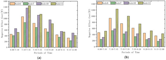
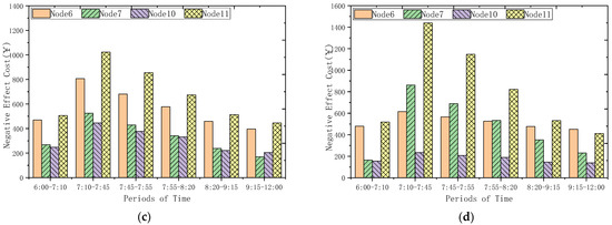
Figure 10.
The negative cost of energy replenishment vehicles during holidays. (a) 10% of the electric vehicle market. (b) 30% of the electric vehicle market. (c) 50% of the electric vehicle market. (d) 80% of the electric vehicle market.
7. Conclusions
On the basis of clarifying the negative effect evaluation method of the energy supply network, the prediction model of the negative effect is established considering the energy replenishing behaviors of electric vehicles and fuel vehicles based on time series data of holidays.
Due to the rush demand for vehicle energy replenishment during holidays, it is impossible to predict the daily energy replenishment flow directly. The traffic flow of vehicle energy replenishment under special demand is obtained through the traffic equilibrium distribution model of mixed users. The Frank–Wolfe algorithm is used to obtain the time period balanced distribution results, and the negative effect cost of vehicle energy replenishment. The results show that the proportion of energy supply resources and travel flow has a significant relationship with the magnitude of the negative impact of energy supply, which is caused by the difference between energy supply and demand. With the continuous tension of energy supply resources, the negative impact increases sharply. Under the same travel flow, with the increase of the penetration rate of electric vehicles, the negative impact of energy supply decreased slowly at first and then increased rapidly. This is due to the excessive number of electric vehicles leading to a long charging queue time, and the negative impact increased significantly.
The energy replenishment efficiency of electric vehicles in charging stations should be well planned. Through the prediction model and its findings, it can provide road traffic optimization ideas for managers and references for the formulation of management schemes so as to alleviate urban traffic problems caused by energy-supplementing vehicles.
Author Contributions
Methodology, X.G.; Investigation, Y.Z.; Data curation, B.W.; Writing—original draft, Z.Y. All authors have read and agreed to the published version of the manuscript.
Funding
This research was funded by the Chongqing graduate Scientific research innovation Project [grant number CYB22239, 2022]. This study was also supported by the General Project of Chongqing Natural Science Foundation [grant number cstc2020jcyj-msxmX0108] and the Key scientific and technological innovation project of “Construction of Chengdu-Chongqing Economic Circle” of Chongqing Municipal Education Commission [grant number KJCXZD2020031].
Institutional Review Board Statement
Not applicable.
Informed Consent Statement
Not applicable.
Data Availability Statement
Not applicable.
Conflicts of Interest
The authors declare no conflict of interest.
References
- Wardorp, J. Some Theoretical Aspects of Road Traffic Research. ICE Proc. Eng. Div. 1952, 1, 767–768. [Google Scholar] [CrossRef]
- Beckmann, M.; McGuire, C.B.; Winsten, C.B. Studies in the Economics of Transportation. Econ. J. 1956, 26, 820–821. [Google Scholar]
- Frank, M.; Wolfe, P. An algorithm for quadratic programming. Nav. Res. Logist. Q. 2010, 3, 95–110. [Google Scholar] [CrossRef]
- Delle Site, P. A mixed-behaviour equilibrium model under predictive and static Advanced Traveller Information Systems (ATIS) and state-dependent route choice. Transp. Res. Part C Emerg. Technol. 2018, 86, 549–562. [Google Scholar] [CrossRef]
- Banadaki, H.D.; Saffarzadeh, M.; Zoghi, H. Developing a Dynamic Traffic Assignment Model for Large-Scale Networks: A Case Study in the City of Yazd, Iran. KSCE J. Civ. Eng. 2021, 25, 3492–3501. [Google Scholar] [CrossRef]
- Friesz, T.L.; Bernstein, D.; Smith, T.E.; Tobin, R.L.; Wie, B.W. A Variational Inequality Formulation of the Dynamic Network User Equilibrium Problem. Oper. Res. 1993, 41, 179–191. [Google Scholar] [CrossRef]
- Friesz, T.L.; Bernstein, D.; Suo, Z.; Tobin, R.L. Dynamic Network User Equilibrium with State-Dependent Time Lags. Netw. Spat. Econ. 2001, 1, 319–347. [Google Scholar] [CrossRef]
- Ye, H.; Xiao, F.; Yang, H. Exploration of day-to-day route choice models by a virtual experiment. Transp. Res. Procedia 2017, 23, 679–699. [Google Scholar] [CrossRef]
- Javani, B.; Babazadeh, A.; Ceder, A. Path-Based Capacity-Restrained Dynamic Traffic Assignment Algorithm. Transp. B 2018, 7, 741–764. [Google Scholar] [CrossRef]
- Cantarella, G.E.; Watling, D.P. A general stochastic process for day-to-day dynamic traffic assignment: Formulation, asymptotic behaviour, and stability analysis. Transp. Res. Part B Methodol. 2016, 92, 3–21. [Google Scholar] [CrossRef]
- Zhao, C.L.; Leclercq, L. Graphical solution for system optimum dynamic traffic assignment with day-based incentive routing strategies. Transp. Res. Part B Methodol. 2018, 117, 87–100. [Google Scholar] [CrossRef]
- Carey, M. Optimal Time-Varying Flows on Congested Networks. Oper. Res. 1987, 35, 58–69. [Google Scholar] [CrossRef]
- He, X.; Liu, H. Modeling the day-to-day traffic evolution process after an unexpected network disruption. Transp. Res. Part B Methodol. 2012, 46, 50–71. [Google Scholar] [CrossRef]
- Long, J.; Chen, J.; Szeto, W.Y.; Shi, Q. Link-based system optimum dynamic traffic assignment problems with environmental objectives. Transp. Res. Part D Transp. Environ. 2016, 60, 56–75. [Google Scholar] [CrossRef]
- Huang, H.-J.; Li, Z.-C. A multiclass, multicriteria logit-based traffic equilibrium assignment model under ATIS. Eur. J. Oper. Res. 2007, 176, 1464–1477. [Google Scholar] [CrossRef]
- Watabe, A.; Leaver, J.; Ishida, H.; Shafiei, E. Impact of low emissions vehicles on reducing greenhouse gas emissions in Japan. Energy Policy 2019, 130, 227–242. [Google Scholar] [CrossRef]
- Smart, J.; Schey, S. Battery Electric Vehicle Driving and Charging Behavior Observed Early in The EV Project. SAE Int. J. Altern. Powertrains 2012, 1, 27–33. [Google Scholar] [CrossRef]
- Cen, X.; Lo, H.K.; Li, L.; Lee, E. Modeling electric vehicles adoption for urban commute trips. Transp. Res. Part B Methodol. 2018, 117, 431–454. [Google Scholar] [CrossRef]
- Lucas, A.; Silva, C.A.; Neto, R.C. Life cycle analysis of energy supply infrastructure for conventional and electric vehicles. Energy Policy 2012, 41, 537–547. [Google Scholar] [CrossRef]
- Ma, D.; Song, X.; Li, P. Daily Traffic Flow Forecasting Through a Contextual Convolutional Recurrent Neural Network Modeling Inter-and Intra-Day Traffic Patterns. IEEE Trans. Intell. Transp. Syst. 2020, 22, 2627–2636. [Google Scholar] [CrossRef]
- Yu, Y.; Han, K.; Ochieng, W. Day-to-Day Dynamic Traffic Assignment with Imperfect Information, Bounded Rationality and Information Sharing. Transp. Res. Part C Emerg. Technol. 2018, 114, 59–83. [Google Scholar] [CrossRef]
- Zhou, S.; Zhuang, Y.; Gu, W.; Wu, Z. Operation and Economic Assessment of Hybrid Refueling Station Considering Traffic Flow Information. Energies 2018, 11, 1991. [Google Scholar] [CrossRef]
- Yeh, S. An empirical analysis on the adoption of alternative fuel vehicles: The case of natural gas vehicles. Inst. Transp. Stud. Work. Pap. Ser. 2007, 35, 5865–5875. [Google Scholar] [CrossRef]
- Zhang, X.; Liu, W.; Waller, S.T. A network traffic assignment model for autonomous vehicles with parking choices. Comput. -Aided Civ. Infrastruct. Eng. 2019, 34, 1100–1118. [Google Scholar] [CrossRef]
- Honma, Y.; Kuby, M. Node-based vs. path-based location models for urban hydrogen refueling stations: Comparing convenience and coverage abilities. Int. J. Hydrogen Energy 2019, 44, 15246–15261. [Google Scholar] [CrossRef]
Disclaimer/Publisher’s Note: The statements, opinions and data contained in all publications are solely those of the individual author(s) and contributor(s) and not of MDPI and/or the editor(s). MDPI and/or the editor(s) disclaim responsibility for any injury to people or property resulting from any ideas, methods, instructions or products referred to in the content. |
© 2023 by the authors. Licensee MDPI, Basel, Switzerland. This article is an open access article distributed under the terms and conditions of the Creative Commons Attribution (CC BY) license (https://creativecommons.org/licenses/by/4.0/).