Article

Intelligent Time Delay Control of Telepresence Robots Using Novel Deep Reinforcement Learning Algorithm to Interact with Patients

1
Electrical Engineering Department, The University of Lahore, Lahore 54000, Pakistan
2
Department of Computer Science, Prince Sattam Bin Abdulaziz University, Al-Kharj 11942, Saudi Arabia
3
Faculty of Computing and Information Technology, King Abdulaziz University, Jeddah 21589, Saudi Arabia
*
Author to whom correspondence should be addressed.
Appl. Sci. 2023, 13(4), 2462; https://doi.org/10.3390/app13042462
Submission received: 15 January 2023 / Revised: 6 February 2023 / Accepted: 10 February 2023 / Published: 14 February 2023

Abstract

:
Telepresence robots are gaining more popularity as a means of remote communication and human–robot interaction, allowing users to control and operate a physical robot remotely. However, controlling these robots can be challenging due to the inherent delays and latency in the communication systems. In this research paper, we propose a novel hybrid algorithm exploiting deep reinforcement learning (DRL) with a dueling double-deep Q-network (DDQN) and a gated recurrent unit (GRU) to assist and maneuver the telepresence robot during the delayed operating signals from the operator. The DDQN is used to learn the optimal control policy for the telepresence robot in a remote healthcare environment during delayed communication signals. In contrast, the GRU is employed to model the control signals’ temporal dependencies and handle the variable time delays in the communication system. The proposed hybrid approach is evaluated analytically and experimentally. The results demonstrate the approach’s effectiveness in improving telepresence robots’ tracking accuracy and stability performance. Multiple experiments show that the proposed technique depicts improved controlling efficiency with no guidance from the teleoperator. It can control and manage the operations of the telepresence robot during the delayed communication of 15 seconds by itself, which is 2.4% better than the existing approaches. Overall, the proposed hybrid approach demonstrates the potential implementation of RL and deep learning techniques in improving the control and stability of the telepresence robot during delayed operating signals from the operator.

1. Introduction

A telepresence robot empowers a distant commanding user to experience real-time presence in remote locations [1]. Cameras are mounted on a robot to recognize the remote environment. A telepresence robot is similar to a mobile robotic system that enables remote users to experience physical mobility. Telemedicine, tele-doctor, telesurgery, and telerehabilitation can save time and money in various tasks. The framework for controlling a telepresence robot combines two-way communication, control signals, and video data, as shown in Figure 1. The telepresence robot operates effectively through signals received from the teleoperator. However, in the event of communication delays, the behavior of the telepresence robot becomes erratic and unpredictable in unfamiliar remote healthcare environments, potentially resulting in collisions and causing harm to individuals. During the period of delayed communication, it may be advantageous to implement an autonomous strategy that effectively assists the telepresence robot. This strategy would involve learning from the teleoperator’s operating behavior and adapting to maneuver efficiently in the remote environment. Simultaneous localization and mapping (SLAM) were one of the compelling algorithms used in mobile robot navigation. The SLAM algorithm uses the input data from different sensors, such as the camera, Lidar, and other sensors, to reconstruct an offline map to understand the surrounding unknown environment [2]. A generalized algorithm flow of a telepresence robot is shown in Figure 2.
The primary issue with the SLAM was using multiple robot sensors to calculate the input data and achieve the estimated environment information to devise the navigation-controlling signal. Visual SLAM [3] navigates by using images as the primary source, but it contains enormous and unnecessary data from the unknown environment and can better recognize the environment. The conventional visual SLAM estimates the camera pose, processes it, and then reconstructs the map. Achieving inter-frame estimations through matching between feature points by extracting image features improves visual SLAM, which has many limitations. Many challenges exist regarding the lack of texture in a single environment and target motion.
Simultaneously, artificial intelligence has introduced the famous direction in respective fields of robot autonomous controlling with deep reinforcement learning (DRL) [4]. The decision-making capability and deep learning control the agent’s actions. The main idea of deep learning (DL) is similar to a human neural network, which is to merge low-level features to form abstract to distinguish high-level representations through multilayered network structures. The primary purpose of reinforcement learning (RL) is to understand the optimum strategy for achieving the objective by increasing the agent’s accumulative reward value acquired from the environment. Hence, RL’s method focuses on learning approaches to resolve complications.
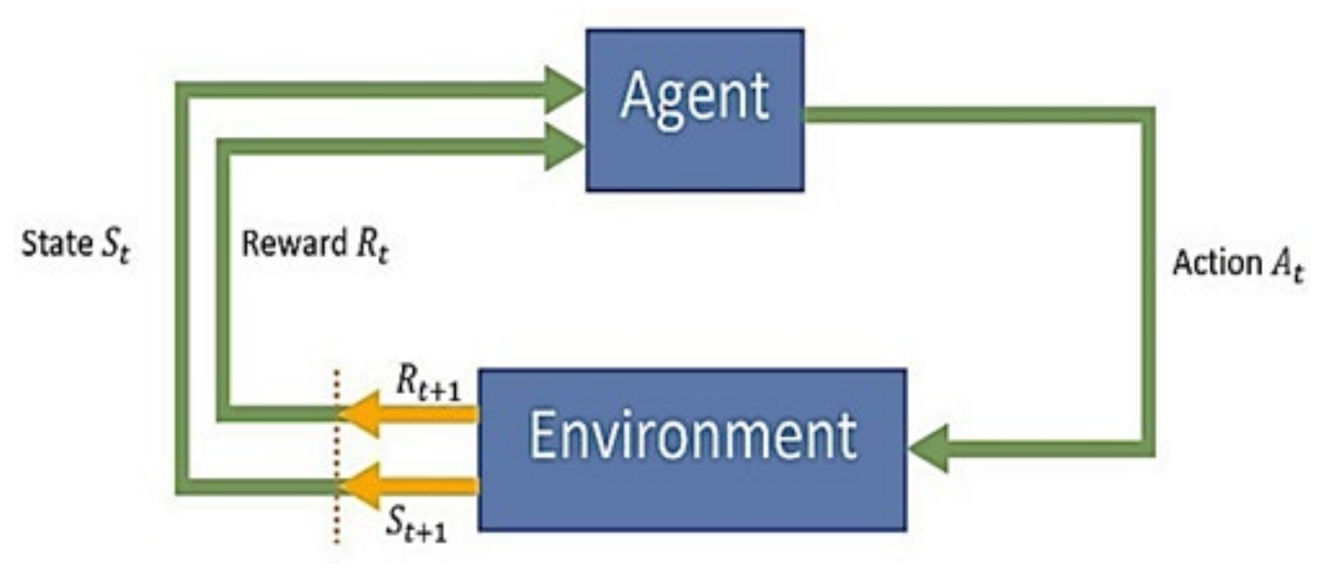
RL is concerned about an agent that discovers how to execute a specific task through trial and error while interacting with unknown environment parameters, which provides feedback regarding reward at the end, as shown in Figure 3. The interaction of the agent and the environment is a continual process. Initially, at time t , an agent receives information about its environment from its sensor’s input s t , based upon which the agent selects an action a t from the set A of the possible actions, then action a t is executed in the environment [5]. The action a t performed in the environment according to the state value s t , and its effect that the agent receives a scalar reward r t + 1 and a new state s t + 1 . The main target of the agent is to maximize the reward it receives from the environment after more trials. Due to this, the agent calculates an action-value function Q ( · ,   · ) that maps state-action pairs into the corresponding expected return. DRL has broadly been used for various applications, including but not limited to computer vision [6,7], robotics [8], natural language processing, video games [9], education, transportation, finance, and healthcare. Zhang et al. proposed a novel danger-aware adaptive composition framework method for self-navigation [10] and a map-less navigation method for robot navigation [11]. Shao, Yan et al. solved a robot navigation problem with the novel method of DRL with a graph attention network (GAT) among external autonomous agents [12].
This paper proposes a complete controlling strategy to assist the teleoperator in an unknown dynamic healthcare environment during delayed operating signals from the operator. The proposed model is tested in the gmapping environment using interfaces based on a robot operating system (ROS), and the outcome shows that the technique is workable and effective.
The primary purpose of our research is to demonstrate a novel hybrid approach consisting of gated recurrent units (GRU) integrated with a double deep Q-learning network (DDQN) algorithm. Then we used it to control differentially driven telepresence robots. With two different input signals, we define the kinematics of the mobile robot. We consider the definition of reward as a variable, the kind of control input, and the random exploratory process to demonstrate the impact on the learning process. This proposed study presents a new method for controlling a telepresence robot with the ability to make autonomous decisions by learning from ongoing controlling signals provided by the teleoperator during delayed communication.
The remaining article is organized as follows: Section 2 discusses the related work and literature review. An overall system overview is presented in Section 3. Section 4 presents the proposed model for controlling the telepresence robot. We discuss the experimental analysis in Section 5, and the Section 6 concludes the article.

2. Related Works

Different approaches discussed in this section have already been used to develop a system to assist in mobile robot teleoperation. As long as the telepresence robot and its delay in communication is a concern, we discuss different related approaches in detail. The telepresence robot’s task is to move around in different dynamic environments ranging from indoor [13] to outdoor, including static to dynamic obstacles [14].
The sample-based approach discretizes the state space and action to transform the main problem of controlling a telerobot into a graphical research task [15] by using pre-computed motion primitives [16]. Additional extensions offer cost functions more suited to the search algorithm. The state grid planner [17] selects a deterministic grid model with the state space. Randomness helps reduce generated trajectories that are irrelevant to a particular search problem. The sampling approach is imperfect but provides probabilistic integrity [18]. In other words, the likelihood of finding a solution increases over time. However, a sample-based system discretizes the state and action space, which requires many computational resources to explain all potential movements. Generally, a large number of motion primitives rapidly increases time complexity.
The interpolation-based method uses waypoints to calculate paths with high path continuity. The more complex approach uses clothoid curves [19], polynomial curves [20], and Bezier curves [21]. The curvature of the clothoid curve uses the arc length and can determine trajectory based on the linear change in curvature. The polynomial curves describe lateral constraints because the constraints of the initial and final segments determine the coefficients.
Numerical optimization creates trajectories based on differentiated cost functions and secondary constraints. Based on the convex function of costs and constraints [22], find the globally optimal trajectory [23]. Optimize the suboptimal orbit [24] or calculate the orbit with a predefined constraint [25]. Continuous trajectories are generated by optimizing functions considering planning parameters such as position, speed, acceleration, and thrust. However, the disadvantage of further optimization steps is the increased complexity of the time. The subsequent best trajectory calculates quickly, but the optimal solution is less applicable to critical tasks and is time-consuming.
Minamoto et al. [26] control the remote robot using an eye-tracking device in a gaze pattern. Compared to manual operation, the time increased to complete the task. In [27] and [28], tactile feedback on environmental forces was obtained for obstacle avoidance by defining virtual environmental forces based on the relative distance and speed between the rover and the obstacle. To better mimic everyday driving, this letter uses the local robot’s extra Degree of Freedom (DOF) as a throttle to control the acceleration of the remote car, making the remote car an obstacle in the environment.
In [29], Zhu, Aoyama, and Hasegawa used fuzzy logic in the remote control operation and obtained good results. The evaluation efficiency of a fuzzy system can effectively overcome simulation errors and noise in the system. As a result, their systems are robust to parameter mismatch model errors, delays, impedance failures, and other uncertainties by adjusting online control parameters in fragile environments.
Spong et al. have suggested a technique of controlling the permanence of the global circuit and guaranteed idle time in remote control systems based on a master-slave. However, if the delay in communication is high, passive loop gain can be reduced [30].
In addition, Kunii et al. offer research on the mobile robot by introducing route plans based on maps of the remote environment along with route adjustments according to the latest measurements from the side of the remote mobile robot. There is a considerable communication delay for planetary observations [31].
Although this method uses a template control to add training data, its effectiveness has not been evaluated in the real world. Sasaki et al. [32] and Vamvoudakis et al. [33] proposed a method of learning a matrix of input coefficients. However, RL linear-quadratic regulator (LQR) inversion has little research on compensating for the undefined behavior of learning methods during actual robot operation.
Anderson et al. [34] proposed a study on the navigation of mobile robots in an indoor environment and accomplished it by using Matterport3D for simulation purposes. Visual input uses to reach the target location. The natural language commands started the navigation procedure. Typically, learning-based navigation is applied using navigation visuals along with DRLs, while using the simulated environments. In Zhu et al. [35], agent navigation was performed using the DRL and visual navigation without a geometric map. AI2-THOR was used as a simulation environment. An image of a natural scene and an image of the target scene are input to the agent. Navigation ends with the agent when the received scene is closely related to the target scene. Yang et al. [36] proposed a technique that used a GCN to obtain semantic information to improve the calculation of the global context model and the relationship between the other objects and targets located in the environment. Learning-based navigation approach with DRL is used in the simulated environment to help the agent navigate successfully by the agent.
Wang [37] proposed a multi-robot coordination algorithm that uses DRL to solve the multi-robot coordination problem. This algorithm resolves source conflicts and avoids obstacles, whose input is an image generated by each robot’s view and reward. This algorithm uses a modified neural network structure based on the neural network battle structure [38]. The dual network structure uses two threads to represent the flag function and the action setting function that, depending on status, combine the results of both streams. The proposed method solves one aspect of resource competition and the noise avoidance problem between static and dynamic multi-robots.
Some 3D scheduling work is performed by using hierarchical control, separating high-level scheduling from low-level motion control and including each in a different neural network [39,40]. Early studies on direct modeling of driving behavior using neural networks [41] focused on studying discrete steering outputs based on layers fully connected to selective downward image streams in neural networks. It was. This approach has been extended in recent studies through Convolutional Neural Networks (CNN) [42] and has significantly scaled to dataset size, task complexity, and performance. [43] proposes real-time path planning to address uncertain dynamics and similar environments by combining a probabilistic roadmap (PRM) with RL.
Q-learning or in-depth Numerous self-driving tasks have been extensively used Q-learning. [44] provided a technique for learning overtaking for simple Q-learning for essential activities. The Q-learning method is used in [45] to teach more advanced actions, including overtaking and blocking. The generalization problem, or learning to pass vehicles that exhibit diverse characteristics, is the focus of surpassing research. When applying Q-learning to these tasks, it is necessary to discretize the basic actions in continuous space into a set of constrained fixed values for control signals. On the other hand, driving a car necessitates more fluid control signals. Planning and control in an ongoing action environment are preferred from the driver’s perspective.
Policy gradient approaches are thought to be more effective than Q-learning and can resolve challenging problems in continuous space [46]. The “Vanilla” policy gradient, likelihood ratio, finite-difference, and natural Actor-Critic approaches are only a few of the policy gradient techniques used in robotics [47]. In [48], authors suggested a deterministic policy gradient algorithm with continuous actions as an alternative to a stochastic policy gradient. By contrast, the training outcomes of Atari games using the two different approaches make the case that a deterministic policy gradient can be far more effective than the conventional stochastic policy gradient. Self-driving cars with simple behaviors are taught how to avoid obstacles via a deep deterministic policy gradient [49]. There are several issues if the policy gradient method is utilized in our jobs.
The advantages and disadvantages of the discussed methods are compared in Table 1.

3. System Development

This section discusses the overall system development, comprises mathematical modeling, 3D modeling, and design of our telepresence robot in detail, and is structured into five sub-sections.

3.1. Telepresence Robot Design

This section will describe the telepresence robot used in this article to gather data for the training of our model, along with the validation of the predictive output. The robot contains four rubber wheels, with two wheels operated by one geared dc motor, and is connected to the wheels by angled gears pressed against each other by a spring. Combining the spring and the angled gears guarantees a constant contact area and, therefore, the instant response between the wheel and the motor. The initial 3D model was designed in AutoCAD software, shown in Figure 4.
The telepresence robots are designed with a sleek and modern aesthetic, incorporating sleek lines and a futuristic look that sets them apart from traditional robotics. The design of a telepresence robot is centered around providing users with an immersive and intuitive experience, allowing them to easily navigate and control the robot as if they were physically present. Some of the key features that contribute to the design of telepresence robots include high-resolution cameras, multiple joints and degrees of freedom, and advanced control systems that allow for smooth and precise movement. Overall, the design of telepresence robots is focused on enabling users to experience the world in a whole new way, breaking down the barriers of distance and bringing people closer together.
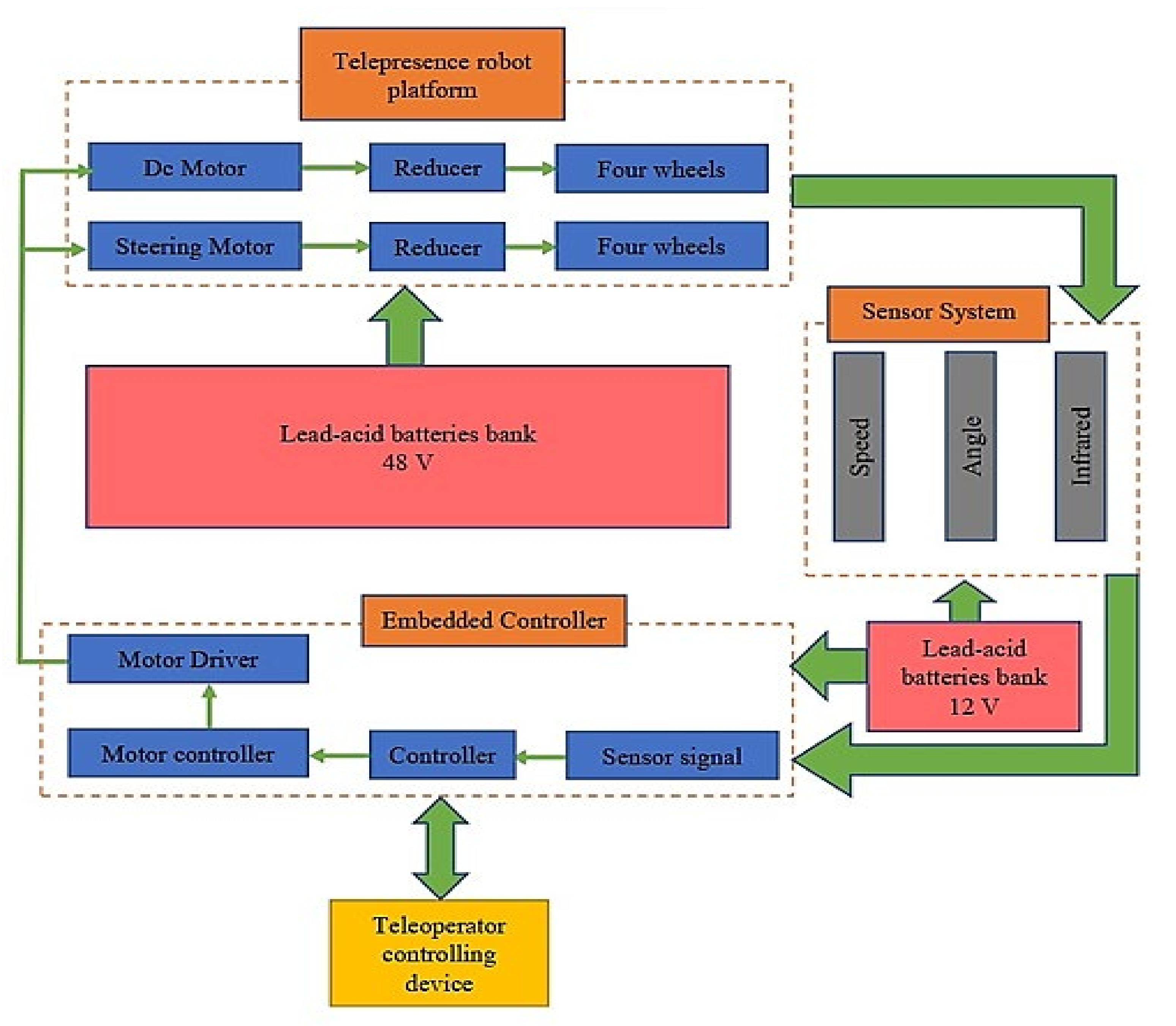
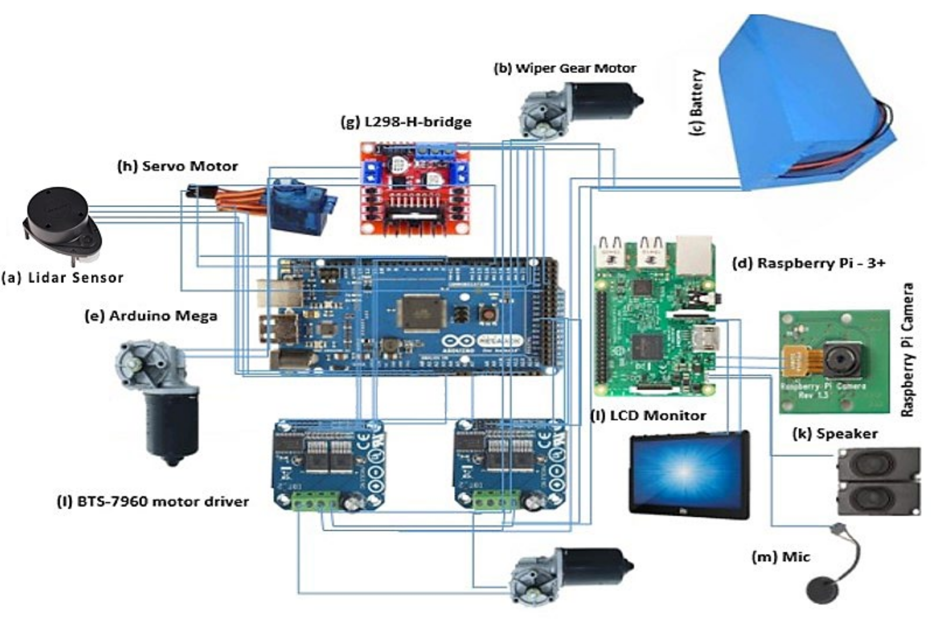
The dc geared motors connect to a motor driver, each being controlled by an Arduino, which in turn receives control signals from a server on a raspberry pi. The same raspberry has a microphone, a speaker connected for audio communication, and a screen to display a commanding user video feed. The raspberry connects to a switch connected to a portable 4G device for internet connectivity to the cloud, and Figure 5 describes the block diagram of our telepresence robot.

3.2. Telepresence Robot Hardware

The hardware components used in the telepresence robot are affordable and easy to find online and in the local market. Every part of the telepresence is manufactured from scratch. Given below is a short description and list of the various components used in it, and it is also shown in Figure 6.

3.2.1. Raspberry Pi Model 3B

At the core of the system, we have used Raspberry Pi. We have used Raspberry Pi 3 Model B, which has 1 GB of RAM, runs at 700 MHz, has 4 USB ports and 1 Ethernet port, and has a total of 40 pins. Twenty-six is the input pin, and the standard output is GPIO and 4 power pins. Two are 5 V, two are 3.3 V, eight are connected to the ground, and two are DoNotConnnect (DNC), so you can program using these pins. All parameters can be used to connect to any sensor inputs, and outputs can be provided by these pins, an HDMI port for screen connection, and power input is a micro USB 5 V 2 A port to load the operating system.

3.2.2. Arduino Mega 2560

Arduino Mega 2560 is a microcontroller board that is designed to be an affordable, user-friendly platform for building electronic projects and prototyping. It is based on the ATmega2560 microcontroller and features a wide range of input/output (I/O) pins, analog inputs, serial ports, and other hardware resources that make it easy to connect sensors, actuators, and other components to the board. The Arduino Mega 2560 can be programmed using the Arduino Integrated Development Environment (IDE) and is compatible with various programming languages, such as C++ and Python.

3.2.3. Arduino Pi Camera

The Raspberry pi camera is an official product of Raspberry pi. It presents the technical specification of a 5 MP camera with a resolution of 2592 × 1944. It uses a camera module weighing around 3 g with an Omnivision OV5647 sensor that connects this sensor to a Raspberry Pi. The Python library extracts parameters from the real-time video feed for image processing.

3.2.4. Motor Driver IBT2-BTS7960

The motor connects to an H-bridge driver module consisting of an Infineon BTS7960 drive chip to protect against overheating and overcurrent. The dual circuitry of the BTS 7960H bridge driver with a powerful drive and braking effect uses the 74HC244 chip to effectively separate the microcontroller and motor driver from a strong current up to 43 A.

3.2.5. Lidar Sensor-RPLiDAR-A1M8-360

Lidar, which stands for Light Detection and Ranging, is a cutting-edge remote sensing technology that uses laser light to map the surface of objects and environments. The basic principle of Lidar is to emit a laser beam toward the target object and measure the time it takes for the laser to return to the system after reflecting off the target. This allows the system to calculate the precise distance to the object and create a detailed 3D map of the environment. Lidar is also increasingly being integrated into telepresence robots, where it plays a crucial role in improving navigation and control. Telepresence robots can be controlled remotely, allowing users to operate a physical robot in a remote environment. Lidar technology provides telepresence robots with the necessary information to navigate their environment and interact with their surroundings, making telepresence robots more effective and efficient in various applications.

3.3. Current Status of Telepresence Robot

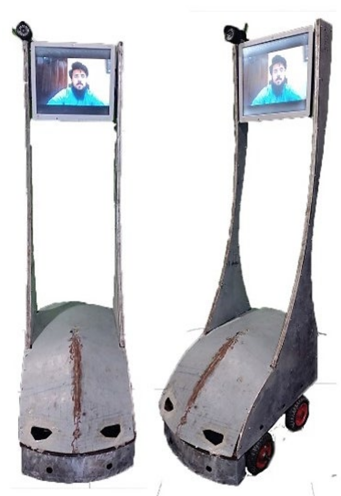
Our telepresence robots are equipped with sensors and a 4G device for internet connectivity to communicate with the remote commanding user. We can now control and maneuver our telepresence robot in an indoor environment. We can move our telepresence robot forward and backward, turn sharp left, turn sharp right, round angled, turn left, and round angled turn right. It is equipped with a pi camera for video transmission, and we can receive the real-time video feed from the telepresence robot to a commanding user display screen. Figure 7 shows the current working telepresence robot.
The purpose of using a telepresence robot prototype for testing and data collection is to simulate a real-world scenario. The robot can be programmed to perform specific tasks, such as navigating through an obstacle course or moving to specific locations, and the results of the proposed approach can be compared with other methods, such as sample-based approaches, interpolation-based methods, numerical optimization, eye-tracking device control, tactile feedback, fuzzy logic, control permanence technique, route plan based on maps, or learning-based navigation. This comparison can help determine the effectiveness and efficiency of the proposed approach in comparison to other methods and provide insight into potential improvements and modifications that can be made.

3.4. Design Parameters of Telepresence Robot

The design parameters of our telepresence robot are triggered by a wheeled motion of a vehicle, such as turning angle, velocity, and angular momentum. The telepresence robot’s parameters are chosen after an analysis of the kinematic motion of the robot, as shown in Table 2.

3.5. Mathematical Modeling of Telepresence Robot

Mathematical models are used to model a system using symbolic computation. This approach helps analyze the dynamics of robots in real-life situations. During the modeling phase, four key components are considered: wheels, bodies, vertical joints, and intelligent devices. Figure 8 shows a schematic representation of the telepresence robot according to the coordinated reference system. The coordinate system for measuring the robot’s position relative to the global reference system for each reference uses a Cartesian coordinate system. Independent coordinates are the vertical displacement x ( t ) and angular rotation θ ( t ) of the wheel, as well as the stresses arising from sliding during horizontal and vertical displacements. To simplify this, we used a 2D model to look at the vertical displacements and rotations of the ramp. Lateral displacement is measured as irrelevant here. Overall lumped gravity central point is chosen in RF 0 and RF 3 in a side view of the diagram.
Nonholonomic is likely the constraint defined in the system. For our telepresence robot, we consider that wheels rotate without slipping, which shows that both wheels have a similar angular rotation, as shown in Equation (1).
φ = R d dt θ w ( t ) = d dt x ( t )
We know that θ w ( t ) is the wheel rotation angle, φ is the steering angle, x ( t ) is the longitudinal translation, and R is the wheel’s radius.
The system’s kinetics is based on the Newton–Euler equation. The unknown variables are solved to derive the grip forces and regular forces. Longitudinal and rotational velocities with varying parameters are given by Equations (2) and (3), according to the symbolic equations.
u ( t ) = d dt x ( t )
u θ ( t ) = d dt θ ( t )
To determine the body weight caused by the upright structure causes the entire robotic platform system to topple concerning the Newton–Euler equations, the Euler equation for the telepresence robot body structure about RF0 and RF3 along with RF6 and RF9 are utilized. The modified equation is as follows in Equation (4).
m tr h d dt u ( t ) + ( 2 m tr h 2 ) L d dt u θ ( t ) m tr h θ ( t ) g = 0
where m tr is the mass of the telepresence robot structure, h is the center of mass, L is the length of the telepresence robot platform (y-axis), as shown in Figure 4, u θ ( t ) is the angular velocity of the robot wheel, and g is the gravitational force constant.
The actual controlling equation of the telepresence robot system is defined in (5), where T c ( t ) is the torque, and M etr represents the equivalent total mass of the telepresence robot. The equivalent value of μ and ψ is given by Equations (6) and (7), respectively.
M etr d dt u ( t ) + μ d dt u θ ( t ) T c ( t ) R + ψ θ ( t ) = 0
μ = ( 2 m tr ( h 2 + hR ) ) RL
ψ = ( ( m tr hg ) R ( 4 m tr h [ u θ ( t ) ] 2 ) L 2 )
The angle of inclinations ( θ ) is a maximum of 35% of the slope. Similarly, the height (h) of the robot support is one of the primary tasks affecting system instabilities.
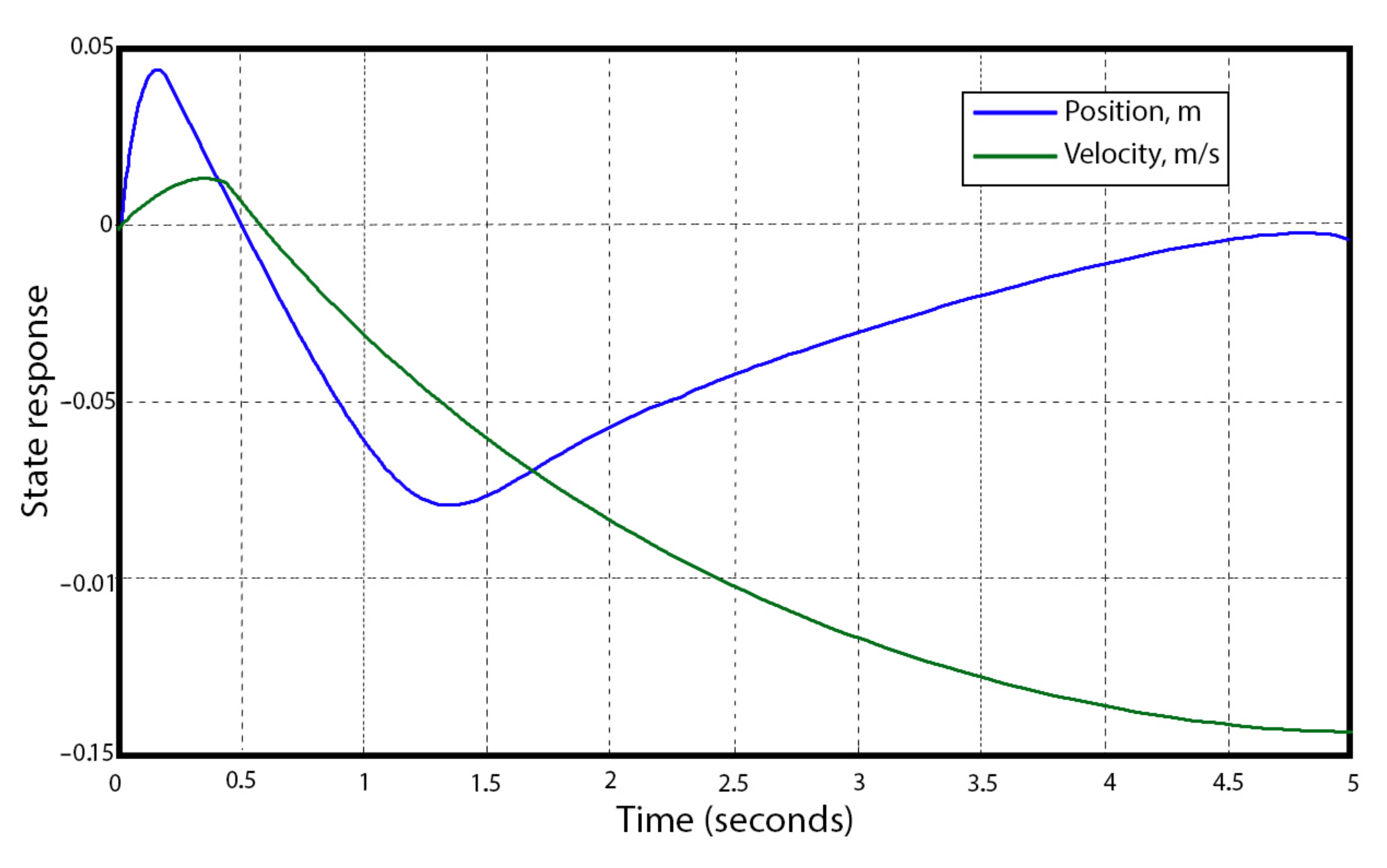
MATLAB simulates the system response and displays it concerning the time interval. With the initial values, the simulation runs for linearized feedback control. According to Figure 9, rotating and steering systems stabilize under 4 s when the angular motion is considered.

4. The Proposed Framework Approach

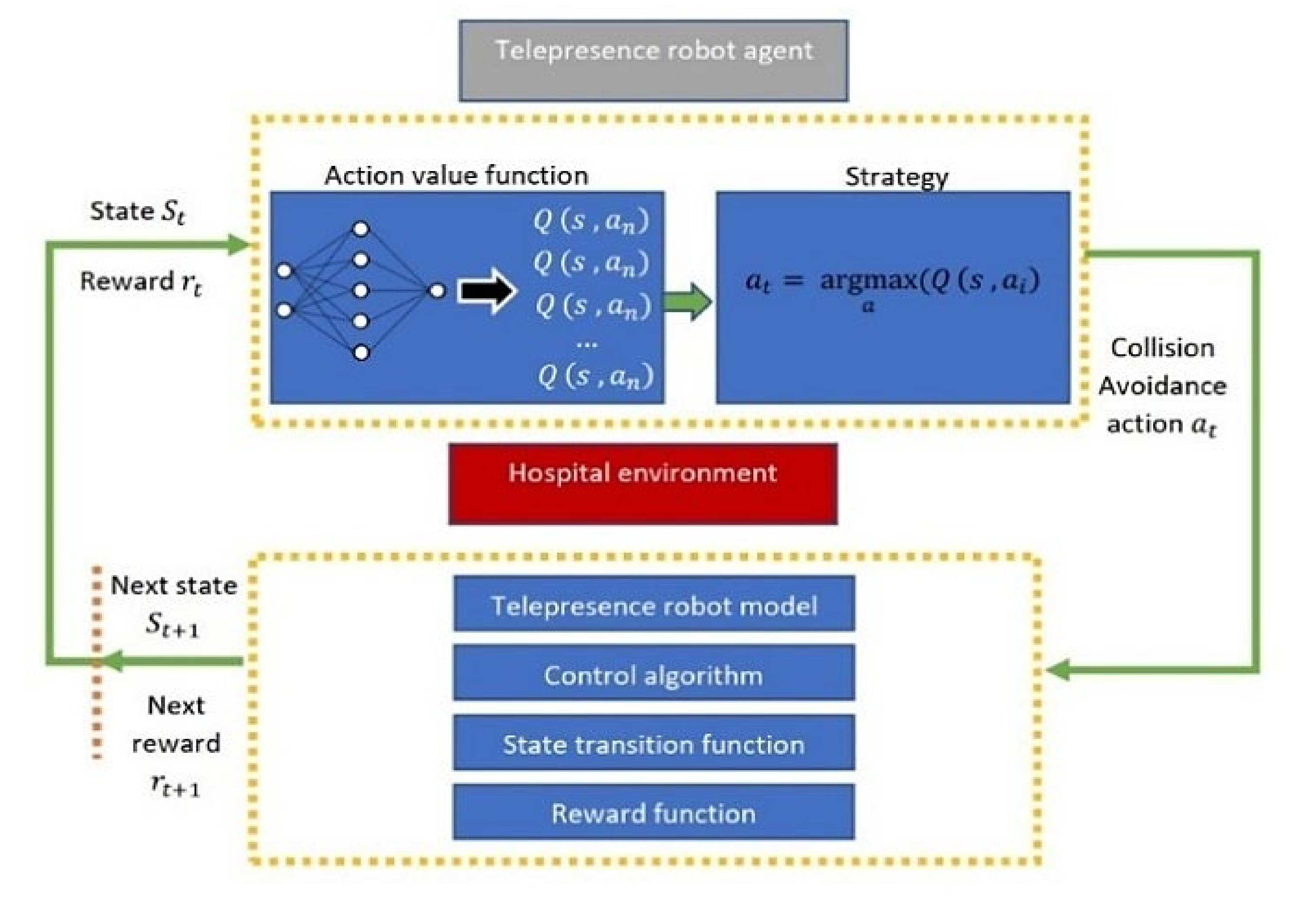
The Proposed approach is to control telepresence robots in assisting with human teleoperators. The primary point of the approach is to design and train a GRU-based DDQN to estimate the agent’s state-action value function. RL is a target-based learning algorithm that can learn and execute decisions autonomously to particular problems. It focuses on agents’ learning by direct interaction with the environment without supervision signals, which is different from other algorithms. The agent performs a mapping of the current scenario into actions so that the agent receives the maximum reward. The agent discovers which actions should be taken to maximize the reward by exploring and trying different actions. The decision-making process affects the immediate gain, the following scenario, and the future return of the actions taken. The essential characteristics of RL are trial and error and delayed gain. The RL system has four significant elements: policy, reward signal, value function, and environment modeling apart from the agent and environment. The reward signal value is the reward given to the developed agent in the form of a value function by the environment. The policy controls system decisions, and the strategy function typically establishes the action, as shown in Figure 10.

4.1. Implementation of the Proposed DRL Framework

This section focuses on maneuvering a telepresence robot in an unfamiliar healthcare environment. This article implements the model of DRL to control the telepresence robot. It initiates with a common neural network with the cyclic neural network of the GRU unit. Furthermore, it merged the DDQN [50] model with the real neural network. The real neural network has enhanced the study by using the GRU [51] unit’s memory ability. The discount factor function, reward value function, and model loss function are more efficient for controlling the telepresence robot. DDQN algorithm is explained in Algorithm 1.
Algorithm 1. Double Deep Q-Networks Learning (DDQN)
1:Initialize: online network Qθ and replay buffer ,
target network Qθ, with weights θ′ ← θ
2:for each episode, do
3:    ovservation of the current state st
4:    for each step in the environment, do
5:        select action a t ~ π ( Q θ ( s t ) ) with respect to the policy π
6:        implement action at
7:        observation of the next state st+1 and reward r t = R ( s t , a t )
8:        store ( s t , a t , s t + 1 , r t in replay buffer
9:        adaptation of the current state st ← st+1
10:      end for
11:    for each update step, do
12:      sample N of experiences with e i = ( s i , a i , s i + 1 , r i ) from replay buffer
13:        calculate expected Q values;
         Q * ( s i , a i ) r i + Υ Q θ ( s i + 1 , argmax a Q θ ( s i + 1 , a ) )
14:        calculate loss L = 1 N i ( Q * ( s i , a i ) Q θ ( s i , a i ) ) 2
15:        calculate the stochastic gradient step on L
16:        updatation of target network parameters:
         θ τ θ + ( 1 τ ) θ
17:    end for
8:end for
Primarily, we need to generate a replay buffer and initialize it online along with target artificial neural networks (ANNs). A duplicate of the online network with identical weights is found in the target network. The agent’s interaction with the environment is represented in the first for-loop, as mentioned in lines 4–10. The learning procedure enabled by the experience replay concept is described in the second for-loop, as mentioned in lines 11–17. The memory storage stores all transactions between the environment and the agent in the form of tuples ( s t ,   a t ,   s t + 1 ,   r t ) is served by the replay buffer , which allows the agent to reuse accumulated experience for better data efficiency.

4.2. Agent Model for Telepresence Robot

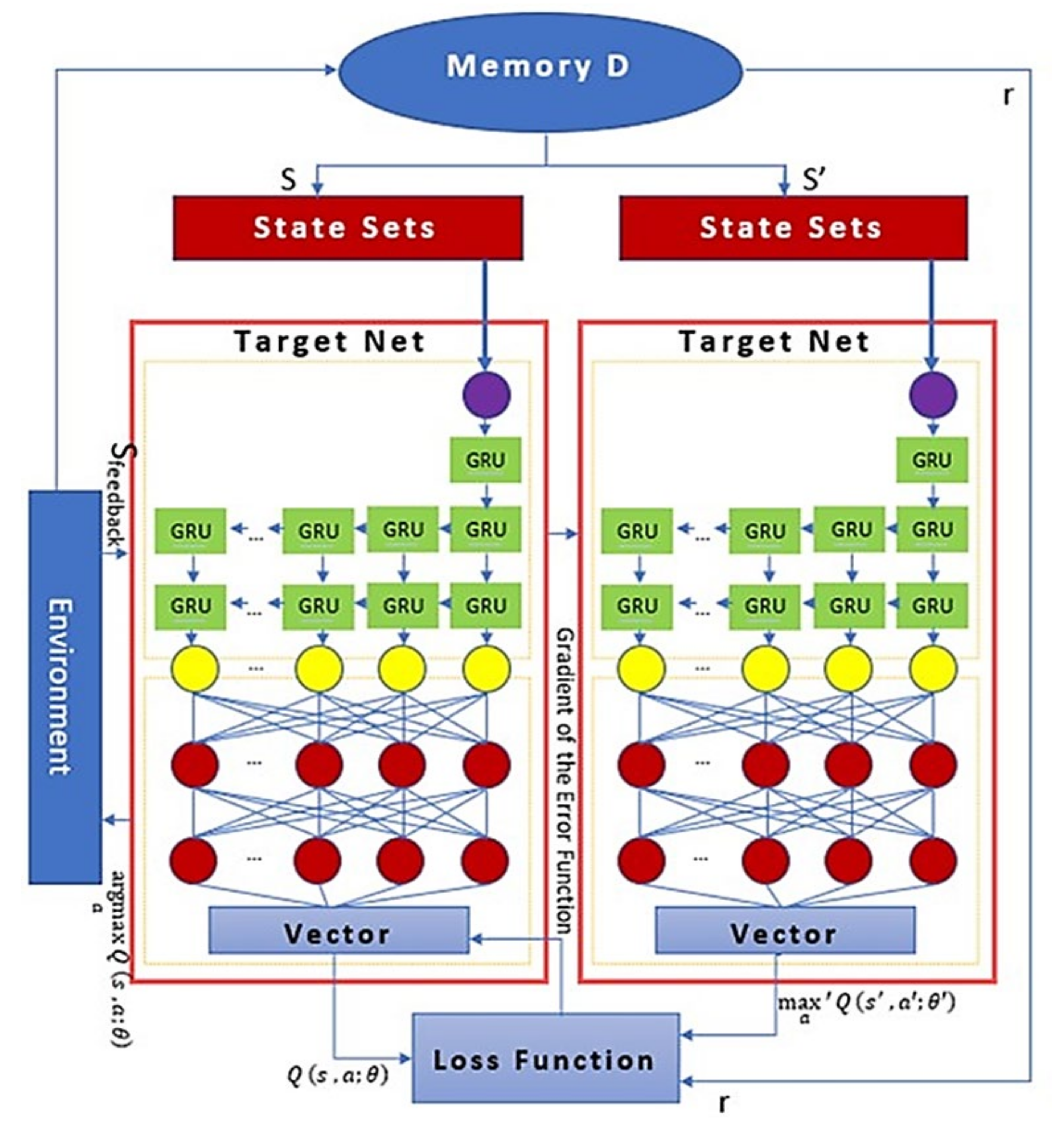
The implementation in this article is based upon double deep q networks (DDQN), which further presents a fully connected (FC) layer and a one-to-many gated recurrent unit (GRU) network layer. The GRU pulls the state’s relevant information to the cell units. The network is a double net frame containing the primary and target networks, as shown in Figure 11. The current state data go to the primary network, and the next state data go to the destination network. Lastly, we use the values acquired from multiple networks, which behave as input to the loss function, to attain the error value.
The revision of each network’s parameter is calculated in the main network, and its synchronization is based on the error gradient. DDQN, with the integration of GRU, supplies the efficient results of training to provide the opportunity of lesser value of loss function and having the idea of better actions. After selecting the final state decision, those related parameters will collect in memory D. We have collected all the state parameters and transmitted the reward value to the loss function. The proposed algorithm is briefly explained in Algorithm 2.
Algorithm 2. Gated Recurrent Unit (GRU) with Double Deep Q-Networks Learning (DDQN)
1: Initialize: input data and Update associated status information ( s , a , r , s ) from memory D,
2: for each episode, do
3:    input will be sent to the main and target networks
4:    input data will send to GRU unit, which has eight behavior sets (columns)
                 A = [ front ,   back ,   left ,   right ,   leftfront ,   rightfront ,   leftrear ,   rightrear ] .
5:    for each step in the GRU unit, do
6:        GRU layers are responsible for processing the n = 8 data
         middle data will be fed to two layers of the FC layer
7:        The FC layer parameter is 8 × 64 and 64 × 8 matrix
        the activation function uses the rectified linear in the neural unit in the FC
        a dropout structure is set in the GRU and FC layers to prevent overfitting
8:    end for
9:    for each update step do
10:        find the action of argmax a Q ( s , a ; θ i )
11:        then
find the action in the target network
12:    The Qtarget value is calculated by using th Q value
13:          The Q value is not certainly the largest in the target network,
          so, we can avoid selecting the overestimated suboptimal action
14:        Memory pool provides the training data
15:        Calculate the loss function:
    L = E { ( r + γ . Q target ( s , argmax a ( Q main ( s , a ) ) ) Q main ( s , a ) ) 2 }
16:    end for
17:end for
Our proposed approach algorithm first retrieves the input data and associated status information from memory module D, which is s , s in the fourth state ( s , a , r , s ) . It expresses the shorthand as (state, action, reward, and next state). Then input will be sent to the main and target networks. The main and target networks are in real-time synchronization, and the network characteristics are identical. The eight-column GRU unit will then receive the input status data. These eight states represent the behavior set in Equation (8).
A = [ front ,   back ,   left ,   right ,   leftfront ,   rightfront ,   leftrear ,   rightrear ]
Three GRU layers are responsible for processing the n = 8 data, after which middle data are fed to two layers of the FC layer. The FC layer parameter structure is 8 × 64 and 64 × 8 matrix, respectively.
1.
The activation function uses the rectified linear in the neural unit in the FC.
2.
A dropout structure is set in the GRU and FC layers to prevent overfitting.
3.
Initially, we find the action of argmax a Q ( s , a ; θ i ) with the main network and then find the action in the target network.
a.
The Q_target value is calculated by using the Q-value.
b.
We can avoid choosing the overstated suboptimal action since the Q value is not unquestionably the highest in the target network.
c.
The memory pool provides the training data.
This article uses the local batch training method known as stochastic gradient descent (SGD). The loss function is given in Equation (9),
L = E { ( r + γ . Q target ( s , argmax a ( Q main ( s , a ) ) ) Q main ( s , a ) ) 2 }
E = 1 N × ( y i y ´ i ) 2
where E in Equation (10) is the error value function, N is the total number of samples, y i is the actual value, and y ´ i is the predicted value. This equation represents the mean squared error (MSE) between the actual and predicted values, which is an error value function in deep reinforcement learning algorithms such as DDQN.

5. Experimental Setup and Results

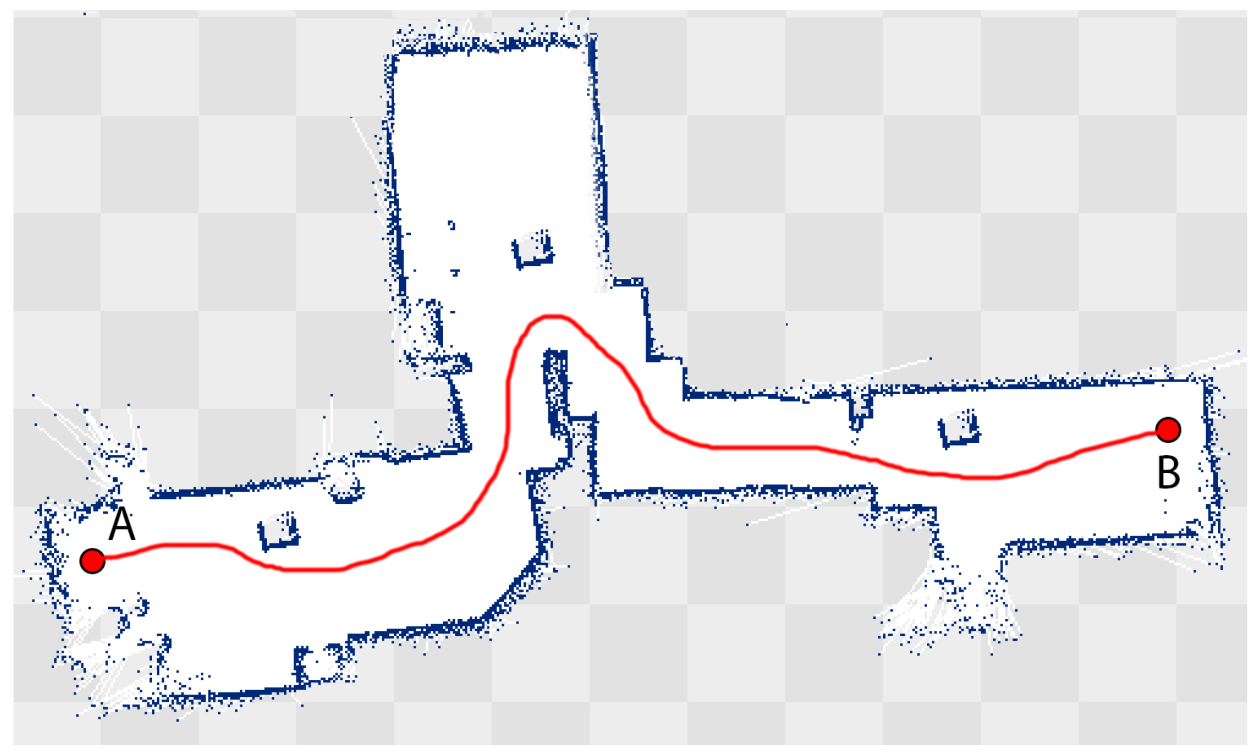
We conducted multiple physical tests on the specially developed telepresence robot using ROS to validate the model’s performance in practice. Numerous tests on the telepresence robot are conducted to reduce the error. The site is a cardiologist ward in the Government general hospital, Ghulam Muhammad-Abad, Faisalabad. The distance for traveling a telepresence robot from the initial point (doctor’s office) to the endpoint (admitted patient ward) is 10.5 m. We use the Lidar to reconstruct the hospital environment. The telepresence robot starts its journey from point A in a hospital environment which is the main entrance of the reception area as shown in Figure 12. It drives through the main lobby while avoiding different static obstacles and reaches destination point B, which is the admitted ward of patients.
Table 3 contains the significant parameters for the experiment environment, which shows the obstacle type: static, and the number of static obstacles is eight and 4 × 4 feet in size. The total coverage path of the telepresence robot from starting A to endpoint B is 140 m. The teleoperator and assistance from the DRL based autonomous are controlling the telepresence robot.
We modify the scanning function to automatic in the gmapping package of ROS to gather the data from the scanner while traveling the telepresence robot from the initial point to the endpoint in the hospital. We performed parameter training based on the hospital environment at the initial stage. Other algorithms have been trained for a certain period except for A*. After receiving all the data, the trained model is fed into the package ROS in the telepresence robot. Then we conducted four verification trips, and each trip was restarted after completing the previous trip. Each trip consists of three different trials, and the mean is established on those trips’ trial data, as discussed in Table 3. By comparing the mean column of the three different trials, the result obtained from the proposed framework-based experiments is good than the other two algorithms’ experiments in the context of trip length and time consumption.
The telepresence robot controlled by the teleoperator makes multiple trips with different measured distance trials from Point A to point B consisting of varying time durations. After learning from the teleoperator-based generated data, and in the scenario of delayed controlling signal, the telepresence robot turns its autonomous mode to move to the desired path by itself. We implement this with three different algorithms, A*, DDQN, and our proposed GRU-integrated DDQN algorithm. We note the cumulative distance covered in a particular time duration, as written in Table 4.
According to this equation, the maximum discounted reward by adhering to that optimal policy for the future state-action pair ( s , a ) will be equal to the predicted reward R t + 1 after executing that action in addition to the optimal Q value function for the given state-activity pair ( s , a ) . The ideal Q value is approximated in a complicated environment using a non-linear function approximator, such as a neural network.
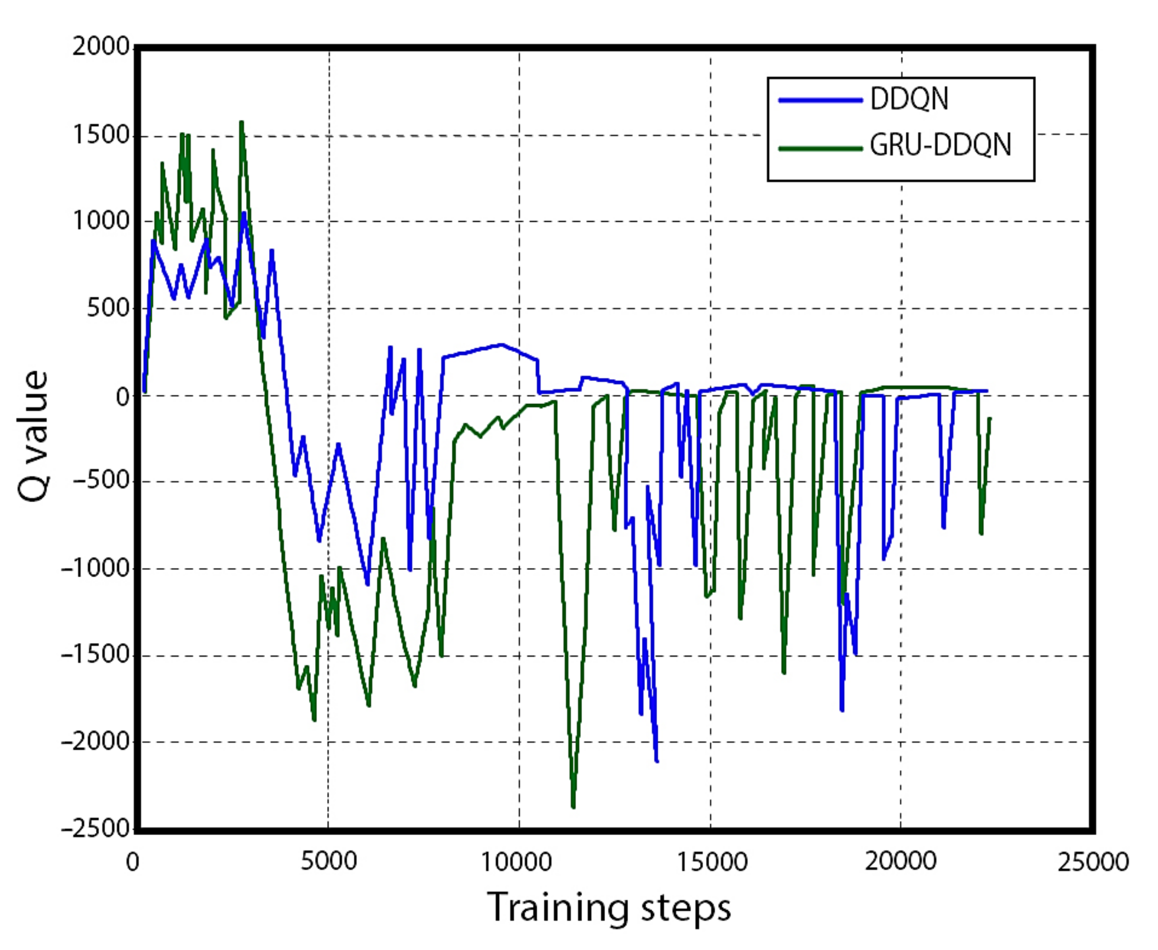
A value-based reinforcement learning technique is called Q-learning. To find the best course of action, Q-learning modifies the Q value of each action-state combination using the Bellman Equation. Furthermore, a dual network structure can lessen the correlation between the present and target Q values and increase the method’s stability. The input value is the state in which each intelligence is present, and the goal function is the Q value corresponding to each action to train the neural network. As shown in Figure 13, the proposed framework has a quicker intersection in the Q value graph after iterations of 4500 training trips compared to the DDQN.
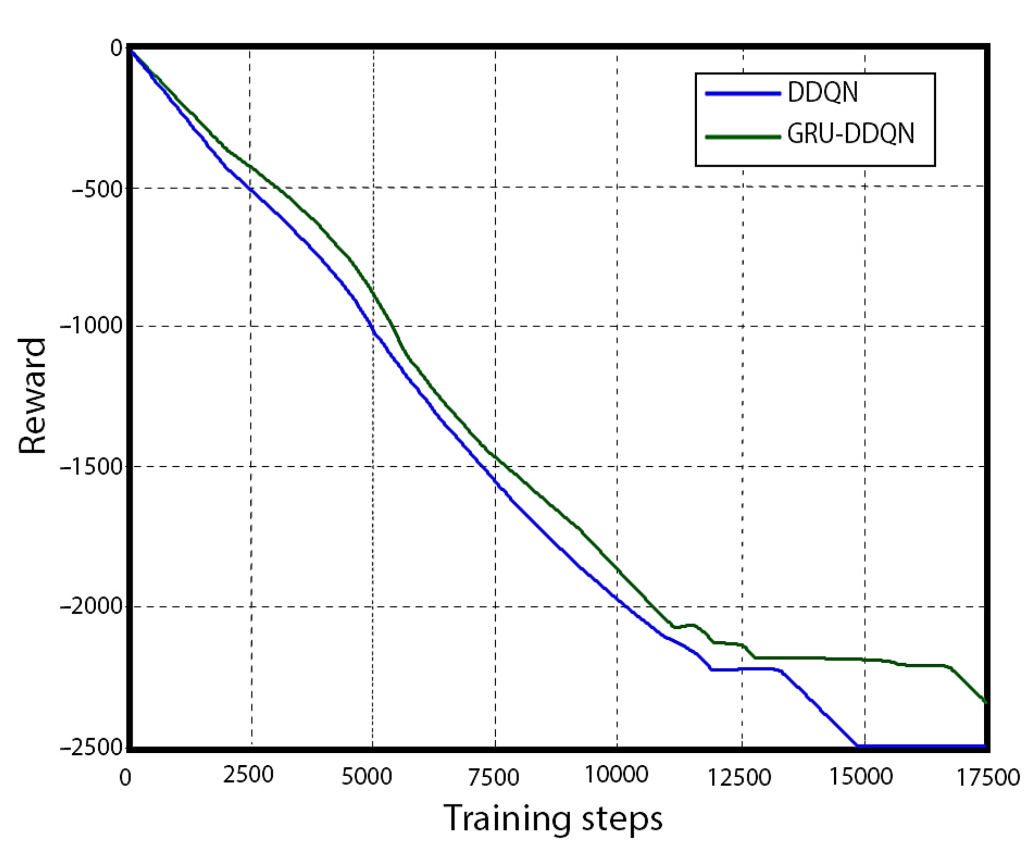
However, it changed abundantly after 1400 tries of training. The proposed framework uses a loop memory network and multiple reward mechanisms compared to DDQN, as shown in Figure 14. In the end, the greater reward value of the proposed framework denotes fewer repeated error-controlling commands.

6. Conclusions

The article implements a DRL-based framework that combines DDQN with the recurrent neural network to control a telepresence robot in unknown environments. The rewards and discount factors are re-designed to improve the controlling method’s feasibility. Experiments show that the different method performs well and makes controlling more efficient. The results after multiple experiments show that the proposed method helps reduce the controlling parameters traveling by 6% compared to other algorithms. In the meantime, the average telepresence robot controlling assistance time duration length is increased by 2.4% as compared to other approaches. Regarding future work, we will implement the other hybrid RL algorithm in telepresence robots to analyze the efficacy of those algorithms in dynamic and complicated environments with active obstacles.

Author Contributions

Conceptualization, F.N. and M.N.K.; methodology, F.N.; software, A.A.; validation, F.N., M.N.K. and A.A.; formal analysis, F.N.; investigation, F.N. and M.N.K.; resources, F.N., M.N.K. and A.A.; data curation, F.N.; writing—original draft preparation, F.N.; writing—review and editing, F.N. and M.N.K.; visualization, F.N., M.N.K. and A.A.; supervis.ion, M.N.K. and A.A.; project administration, M.N.K.; funding acquisition, A.A. All authors have read and agreed to the published version of the manuscript.

Funding

The authors extend their appreciation to the Deputyship for Research and Innovation, the Ministry of Education in Saudi Arabia for funding this research work through the project number IF2/PSAU/2022/01/22378.

Institutional Review Board Statement

This article does not contain any studies with human participants performed by any of the authors.

Informed Consent Statement

Not applicable.

Data Availability Statement

Data sharing not applicable to this article as no datasets were generated during the current study.

Conflicts of Interest

The authors declare no conflict of interest. The manuscript was written through contributions of all authors.

References

  1. Tachi, S. Telexistence. In Lecture Notes in Computer Science; Springer International Publishing: Cham, Switzerland, 2015; pp. 229–259. [Google Scholar] [CrossRef]
  2. Engel, J.; Schöps, T.; Cremers, D. LSD-SLAM: Large-Scale Direct Monocular SLAM. In Computer Vision—ECCV 2014; Springer International Publishing: Cham, Switzerland, 2014; pp. 834–849. [Google Scholar] [CrossRef]
  3. Mur-Artal, R.; Montiel, J.M.M.; Tardos, J.D. ORB-SLAM: A Versatile and Accurate Monocular SLAM System. IEEE Trans. Robot. 2015, 31, 1147–1163. [Google Scholar] [CrossRef]
  4. Zhao, K.; Song, J.; Luo, Y.; Liu, Y. Research on Game-Playing Agents Based on Deep Reinforcement Learning. Robotics 2022, 11, 35. [Google Scholar] [CrossRef]
  5. Jiang, Y.; Shin, H.; Ko, H. Precise Regression for Bounding Box Correction for Improved Tracking Based on Deep Reinforcement Learning. In Proceedings of the ICASSP 2018—2018 IEEE International Conference on Acoustics, Speech and Signal Processing (ICASSP), Calgary, AB, Canada, 15–20 April 2018. [Google Scholar] [CrossRef]
  6. Caicedo, J.C.; Lazebnik, S. Active Object Localization with Deep Reinforcement Learning. In Proceedings of the 2015 IEEE International Conference on Computer Vision (ICCV), Santiago, Chile, 7–13 December 2015. [Google Scholar] [CrossRef]
  7. Ranjith Rochan, M.; Aarthi Alagammai, K.; Sujatha, J. Computer Vision Based Novel Steering Angle Calculation for Autonomous Vehicles. In Proceedings of the 2018 Second IEEE International Conference on Robotic Computing (IRC), Laguna Hills, CA, USA, 31 January–2 February 2018. [Google Scholar] [CrossRef]
  8. Lillicrap, T.P.; Hunt, J.J.; Pritzel, A.; Heess, N.; Erez, T.; Tassa, Y.; Silver, D.; Wierstra, D. Continuous Control with Deep Reinforcement Learning. Comput. Sci. 2015, 8, A187. [Google Scholar]
  9. Hosu, I.-A.; Rebedea, T. Playing Atari Games with Deep Reinforcement Learning and Human Checkpoint Replay. Computer Science. arXiv 2016, arXiv:1607.05077. [Google Scholar]
  10. Zhang, W.; Zhang, Y.; Liu, N. Danger-Aware Adaptive Composition of DRL Agents for Self-Navigation. Unmanned Syst. 2020, 9, 1–9. [Google Scholar] [CrossRef]
  11. Dobrevski, M.; Skočaj, D. Deep reinforcement learning for map-less goal-driven robot navigation. Int. J. Adv. Robot. Syst. 2021, 18, 172988142199262. [Google Scholar] [CrossRef]
  12. Shao, Y.; Li, R.; Zhao, Z.; Zhang, H. Graph Attention Network-based DRL for Network Slicing Management in Dense Cellular Networks. In Proceedings of the 2021 IEEE Wireless Communications and Networking Conference (WCNC), Nanjing, China, 29 March–1 April 2021. [Google Scholar] [CrossRef]
  13. Kebria, P.M.; Khosravi, A.; Nahavandi, S.; Shi, P.; Alizadehsani, R. Robust Adaptive Control Scheme for Teleoperation Systems with Delay and Uncertainties. IEEE Trans. Cybern. 2020, 50, 3243–3253. [Google Scholar] [CrossRef]
  14. Shen, S.; Michael, N.; Kumar, V. Autonomous multi-floor indoor navigation with a computationally constrained MAV. In Proceedings of the 2011 IEEE International Conference on Robotics and Automation (ICRA), Shanghai, China, 9–13 May 2011; IEEE: Piscataway, NJ, USA, 2011. [Google Scholar] [CrossRef]
  15. Likhachev, M.; Ferguson, D.; Gordon, G.; Stentz, A.; Thrun, S. Anytime search in dynamic graphs. Artif. Intell. 2008, 172, 1613–1643. [Google Scholar] [CrossRef]
  16. Howard, T.M.; Green, C.J.; Kelly, A.; Ferguson, D. State space sampling of feasible motions for high-performance mobile robot navigation in complex environments. J. Field Robot. 2008, 25, 325–345. [Google Scholar] [CrossRef]
  17. Wang, S. State Lattice-Based Motion Planning for Autonomous On-Road Driving/Shuiying Wang; Online-Ressource; Freie Universität Berlin: Berlin, Germany, 2015; Available online: http://d-nb.info/1069105651/34 (accessed on 15 January 2023).
  18. Hsu, D.; Latombe, J.-C.; Kurniawati, H. On the Probabilistic Foundations of Probabilistic Roadmap Planning. Int. J. Robot. Res. 2006, 25, 627–643. [Google Scholar] [CrossRef]
  19. Brezak, M.; Petrovic, I. Real-time Approximation of Clothoids With Bounded Error for Path Planning Applications. IEEE Trans. Robot. 2014, 30, 507–515. [Google Scholar] [CrossRef]
  20. Glaser, S.; Vanholme, B.; Mammar, S.; Gruyer, D.; Nouveliere, L. Maneuver-Based Trajectory Planning for Highly Autonomous Vehicles on Real Road with Traffic and Driver Interaction. IEEE Trans. Intell. Transp. Syst. 2010, 11, 589–606. [Google Scholar] [CrossRef]
  21. Rastelli, J.P.; Lattarulo, R.; Nashashibi, F. Dynamic trajectory generation using continuous-curvature algorithms for door to door assistance vehicles. In Proceedings of the 2014 IEEE Intelligent Vehicles Symposium (IV), Dearborn, MI, USA, 8–11 June 2014. [Google Scholar] [CrossRef]
  22. Lim, W.; Lee, S.; Sunwoo, M.; Jo, K. Hierarchical Trajectory Planning of an Autonomous Car Based on the Integration of a Sampling and an Optimization Method. IEEE Trans. Intell. Transp. Syst. 2018, 19, 613–626. [Google Scholar] [CrossRef]
  23. Ziegler, J.; Bender, P.; Dang, T.; Stiller, C. Trajectory planning for Bertha—A local, continuous method. In Proceedings of the 2014 IEEE Intelligent Vehicles Symposium (IV), Dearborn, MI, USA, 8–11 June 2014. [Google Scholar] [CrossRef]
  24. Dolgov, D.; Thrun, S.; Montemerlo, M.; Diebel, J. Path Planning for Autonomous Vehicles in Unknown Semi-structured Environments. Int. J. Robot. Res. 2010, 29, 485–501. [Google Scholar] [CrossRef]
  25. Ziegler, J.; Bender, P.; Schreiber, M.; Lategahn, H.; Strauss, T.; Stiller, C.; Thao, D.; Franke, U.; Appenrodt, N.; Keller, C.G.; et al. Making Bertha Drive—An Autonomous Journey on a Historic Route. IEEE Intell. Transp. Syst. Mag. 2014, 6, 8–20. [Google Scholar] [CrossRef]
  26. Minamoto, M.; Suzuki, Y.; Kanno, T.; Kawashima, K. Effect of robot operation by a camera with the eye tracking control. In Proceedings of the 2017 IEEE International Conference on Mechatronics and Automation (ICMA), Takamatsu, Japan, 6–9 August 2017. [Google Scholar] [CrossRef]
  27. Ma, L.; Xu, Z.; Schilling, K. Robust bilateral teleoperation of a car-like rover with communication delay. In Proceedings of the 2009 European Control Conference (ECC), Budapest, Hungary, 23–26 August 2009. [Google Scholar] [CrossRef]
  28. Xu, Z.; Ma, L.; Schilling, K. Passive bilateral teleoperation of a car-like mobile robot. In Proceedings of the 2009 17th Mediterranean Conference on Control and Automation (MED), Thessaloniki, Greece, 24–26 June 2009. [Google Scholar] [CrossRef]
  29. Zhu, Y.; Aoyama, T.; Hasegawa, Y. Enhancing the Transparency by Onomatopoeia for Passivity-Based Time-Delayed Teleoperation. IEEE Robot. Autom. Lett. 2020, 5, 2981–2986. [Google Scholar] [CrossRef]
  30. Lee, D.; Spong, M.W. Passive Bilateral Teleoperation with Constant Time Delay. IEEE Trans. Robot. 2006, 22, 269–281. [Google Scholar] [CrossRef]
  31. Kunii, Y.; Kubota, T. Human Machine Cooperative Tele-Drive by Path Compensation for Long Range Traversability. In Proceedings of the 2006 IEEE/RSJ International Conference on Intelligent Robots and Systems, Beijing, China, 9–15 October 2006. [Google Scholar] [CrossRef]
  32. Sasaki, T.; Uchibe, E.; Iwane, H.; Yanami, H.; Anai, H.; Doya, K. Policy gradient reinforcement learning method for discrete-time linear quadratic regulation problem using estimated state value function. In Proceedings of the 2017 56th Annual Conference of the Society of Instrument and Control Engineers of Japan (SICE), Kanazawa, Japan, 19–22 September 2017. [Google Scholar] [CrossRef]
  33. Vamvoudakis, K.G.; Modares, H.; Kiumarsi, B.; Lewis, F.L. Game Theory-Based Control System Algorithms with Real-Time Reinforcement Learning: How to Solve Multiplayer Games Online. IEEE Control. Syst. 2017, 37, 33–52. [Google Scholar] [CrossRef]
  34. Anderson, P.; Wu, Q.; Teney, D.; Bruce, J.; Johnson, M.; Sunderhauf, N.; Reid, I.; Gould, S.; van den Hengel, A. Vision-and-Language Navigation: Interpreting Visually-Grounded Navigation Instructions in Real Environments. In Proceedings of the 2018 IEEE/CVF Conference on Computer Vision and Pattern Recognition (CVPR), Salt Lake City, UT, USA, 18–23 June 2018. [Google Scholar] [CrossRef]
  35. Zhu, Y.; Mottaghi, R.; Kolve, E.; Lim, J.J.; Gupta, A.; Fei-Fei, L.; Farhadi, A. Target-driven visual navigation in indoor scenes using deep reinforcement learning. In Proceedings of the 2017 IEEE International Conference on Robotics and Automation (ICRA), Singapore, 29 May–3 June 2017. [Google Scholar] [CrossRef]
  36. Yang, W.; Wang, X.; Farhadi, A.; Gupta, A.; Mottaghi, R. Visual Semantic Navigation using Scene Priors. arXiv 2018, arXiv:1810.06543. [Google Scholar]
  37. Wang, D.; Deng, H.; Pan, Z. MRCDRL: Multi-robot coordination with deep reinforcement learning. Neurocomputing 2020, 406, 68–76. [Google Scholar] [CrossRef]
  38. Wang, Z.; Schaul, T.; Hessel, M.; van Hasselt, H.; Lanctot, M.; de Freitas, N. Dueling Network Architectures for Deep Reinforcement Learning. arXiv 2015, arXiv:1511.06581. [Google Scholar]
  39. Peng, X.B.; Berseth, G.; Yin, K.; Van De Panne, M. DeepLoco: Dynamic locomotion skills using hierarchical deep reinforcement learning. ACM Trans. Graph. 2017, 36, 1–13. [Google Scholar] [CrossRef]
  40. Merel, J.; Ahuja, A.; Pham, V.; Tunyasuvunakool, S.; Liu, S.; Tirumala, D.; Heess, N.; Wayne, G. Hierarchical Visuomotor Control of Humanoids. arXiv 2018, arXiv:1811.09656. [Google Scholar]
  41. Pomerleau, D.A. Neural Network Based Autonomous Navigation. In The Kluwer International Series in Engineering and Computer Science; Springer US: Boston, MA, USA, 1990; pp. 83–93. [Google Scholar] [CrossRef]
  42. Sermanet, P.; Eigen, D.; Zhang, X.; Mathieu, M.; Fergus, R.; LeCun, Y. OverFeat: Integrated Recognition, Localization, and Detection using Convolutional Networks. arXiv 2013, arXiv:1312.6229. [Google Scholar]
  43. Park, J.J.; Kim, J.H.; Song, J.B. Path Planning for a Robot Manipulator Based on Probabilistic Roadmap and Reinforcement Learning. Int. J. Control. Autom. Syst. 2007, 5, 674–680. [Google Scholar]
  44. Loiacono, D.; Prete, A.; Lanzi, P.L.; Cardamone, L. Learning to overtake in TORCS using simple reinforcement learning. In Proceedings of the 2010 IEEE Congress on Evolutionary Computation (CEC), Barcelona, Spain, 18–23 July 2010. [Google Scholar] [CrossRef]
  45. Huang, H.-H.; Wang, T. Learning overtaking and blocking skills in simulated car racing. In Proceedings of the 2015 IEEE Conference on Computational Intelligence and Games (CIG), Tainan, Taiwan, 31 August–2 September 2015. [Google Scholar] [CrossRef]
  46. Karpathy, A. Deep Reinforcement Learning: Pong from Pixels, 31 May 2016. Available online: http://karpathy.github.io/2016/05/31/rl/ (accessed on 18 October 2022).
  47. Peters, J.; Schaal, S. Policy Gradient Methods for Robotics. In Proceedings of the 2006 IEEE/RSJ International Conference on Intelligent Robots and Systems, Beijing, China, 9–15 October 2006. [Google Scholar] [CrossRef]
  48. Silver, D.; Lever, G.; Heess, N.; Degris, T.; Wierstra, D.; Riedmiller, M. Deterministic Policy Gradient Algorithms. In Proceedings of the 31st International Conference on Machine Learning, PMLR, Beijing, China, 22–24 June 2014; Volume 32, pp. 387–395. [Google Scholar]
  49. Zong, X.; Xu, G.; Yu, G.; Su, H.; Hu, C. Obstacle Avoidance for Self-Driving Vehicle with Reinforcement Learning. SAE Int. J. Passeng. Cars Electron. Electr. Syst. 2017, 11, 30–39. [Google Scholar] [CrossRef]
  50. Zhang, X.; Shi, X.; Zhang, Z.; Wang, Z.; Zhang, L. A DDQN Path Planning Algorithm Based on Experience Classification and Multi Steps for Mobile Robots. Electronics 2022, 11, 2120. [Google Scholar] [CrossRef]
  51. Dey, R.; Salem, F.M. Gate-variants of Gated Recurrent Unit (GRU) neural networks. In Proceedings of the 2017 IEEE 60th International Midwest Symposium on Circuits and Systems (MWSCAS), Boston, MA, USA, 6–9 August 2017. [Google Scholar] [CrossRef] [Green Version]
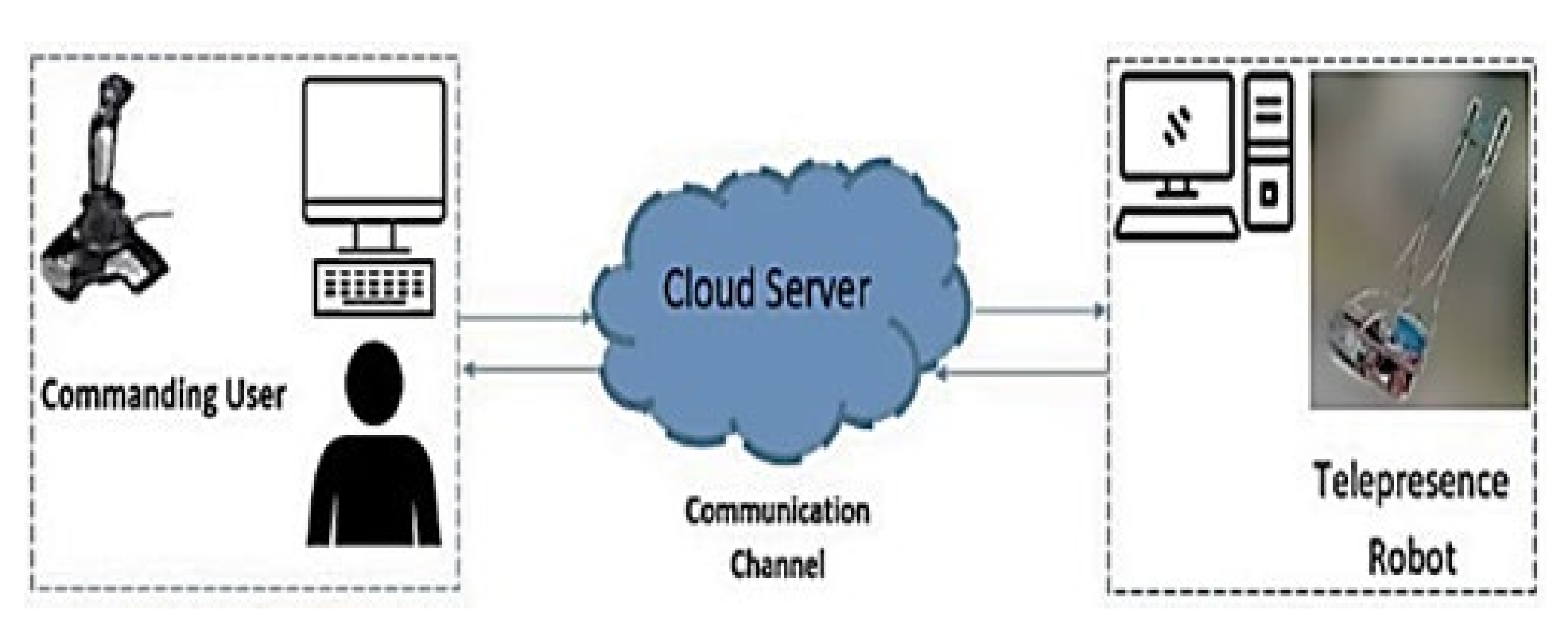
Figure 1. Generalized telepresence robot framework.
Applsci 13 02462 g001
Figure 2. Generalized algorithm flow of a remote-controlled telepresence robot.
Applsci 13 02462 g002
Figure 3. Flow of reinforcement learning.
Applsci 13 02462 g003
Figure 4. Three-dimensional Model of Telepresence Robot.
Applsci 13 02462 g004
Figure 5. System Block Diagram of Telepresence Robot.
Applsci 13 02462 g005
Figure 6. Electronics Component-based Circuit Diagram.
Applsci 13 02462 g006
Figure 7. Manufactured Working Telepresence Robot Prototype. Our telepresence robot prototype is a robotic platform designed to facilitate remote communication and control in real-time. The proposed approach of the hybrid of DDQN and GRU can be implemented and tested on our manufactured robot to gather data and compare its performance with other approaches. The telepresence robot typically includes cameras, sensors, and actuators that allow a remote user to view and interact with the physical environment. The robot’s movement and actions can be controlled through a user interface, such as a joystick, keyboard, or touch screen.
Applsci 13 02462 g007
Figure 8. Schematic representation of telepresence robot.
Applsci 13 02462 g008
Figure 9. Linearized feedback control response with the initial values.
Applsci 13 02462 g009
Figure 10. Proposed approach to control telepresence robot in assistance with human teleoperator.
Applsci 13 02462 g010
Figure 11. Proposed framework based on integration of Gated Recurrent Unit (GRU) with Double Deep Q-learning Network (DDQN).
Applsci 13 02462 g011
Figure 12. Lidar-based indoor map of the hospital and path of a telepresence robot.
Applsci 13 02462 g012
Figure 13. Q value comparison of different approaches.
Applsci 13 02462 g013
Figure 14. Reward comparison of different approaches.
Applsci 13 02462 g014
Table 1. Comparison of few above-mentioned referenced approaches.
Reference ApproachAdvantagesDisadvantages
Sample-BasedProbabilistic integrityDiscretizes state and action space, high time complexity
Interpolation-BasedHigh path continuityComplex approach
Numerical OptimizationGlobally optimal trajectoryIncreased complexity and time-consuming
Fuzzy LogicRobust to uncertaintiesLess precise
Master-SlaveGuaranteed idle timeHigh delay in communication reduces passive loop gain
Route PlanningEffective in remote environmentConsiderable communication delay
Learning-based NavigationImproved navigationLittle research on compensating for undefined behavior during actual operation
DRLEffective in multi-robot coordinationComputational complex
Proposed ApproachMore dynamic and efficient methodLarge Data requirement
Table 2. Telepresence robot parameters.
Technical SpecificationUnitMin–Max Value
Robot speedm/s0–3.25
Robot momentumN.m0–0.93
Robot heightft5′3″
Robot widthft1′5″
Robot breadthft0′6″
Robot weightkg14
Robot batteryAh35
Table 3. Experimental significant parameters.
ParametersUnitValue
Static obstacles4 × 4 feet8
Dynamic Obstacle--
PathCurved1
Starting Point-A (Main entrance)
End Point-B (Patient Ward)
Coverage meters140
Table 4. Experimental data of A*, DDQN and the proposed framework algorithm.
AlgorithmExamplesTrial 1Trial 2Trial 3Mean
Distance (m)/time (s)Distance (m)/time (s)Distance (m)/time (s)Distance (m)/time (s)
A*First trip8.7 m/91 s9.9 m/99 s9.1 m/95 s9.2 m/95 s
Second trip9.9 m/90 s9.1 m/87 s8.1 m/88 s9.0 m/88 s
Third trip9.1 m/98 s9.0 m/89 s9.0 m/75 s9.0 m/87 s
Fourth trip8.4 m/87 s9.8 m/72 s9.9 m/61 s9.3 m/73 s
DDQNFirst trip8.8 m/84 s9.6 m/76 s8.9 m/95 s9.1 m/85 s
Second trip8.4 m/86 s7.8 m/87 s7.9 m/88 s8.0 m/87 s
Third trip9.1 m/80 s8.4 m/79 s8.3 m/75 s8.6 m/78 s
Fourth trip9.0 m/77 s7.9 m/61 s7.8 m/58 s8.2 m/65 s
Proposed FrameworkFirst trip8.1 m/84 s8.8 m/89 s7.7 m/85 s8.2 m/86 s
Second trip7.8 m/86 s7.5 m/87 s8.1 m/88 s7.8 m/87 s
Third trip8.5 m/85 s8.4 m/79 s7.7 m/75 s8.2 m/79 s
Fourth trip7.9 m/73 s8.1 m/69 s7.3 m/71 s7.7 m/71 s
Disclaimer/Publisher’s Note: The statements, opinions and data contained in all publications are solely those of the individual author(s) and contributor(s) and not of MDPI and/or the editor(s). MDPI and/or the editor(s) disclaim responsibility for any injury to people or property resulting from any ideas, methods, instructions or products referred to in the content.