Abstract
Climate change will greatly influence the world at several levels and will have consequences on the interior climate of historic buildings and artifacts conservation. Buildings are responsible for a large slice of the overall emissions, which is due both to the greenhouse gases that are released during their construction as well as the activities that are performed therewithin. One way of counteracting this trend is to design more efficient retrofit buildings and predict their behavior using simulation software, which can thoroughly assess the performance of new buildings or the impact of each retrofit measure for existing buildings. In this study, a calibrated computational model of high thermal inertia building was used to assess the performance of passive retrofits in mitigating the effects of climate change concerning artifact decay mechanisms. In addition, a methodology that aims to reduce the amount of time spent to perform these studies is also presented, in which time savings reach up to 63%.
1. Introduction
1.1. Retrofitting Historic Buildings for the Future Climatic Conditions
The emission of greenhouse gases (GHGs) into the atmosphere caused by anthropogenic activities is greatly responsible for the changes that the outdoor climate will suffer in the future [1]. Climate change is one of the key challenges that mankind faces nowadays since it will greatly influence the environment, human health, and the world’s economy [2]. The European Union (EU) has a key contribution to the overall GHGs emissions since it is responsible for more than one-third of the GHGs emitted by the OECD members, i.e., 5,600,000 tons of CO2-equiv per year [3]. This amount has been steadily decreasing over the past years, mostly due to the efforts made by the EU parliament to promote a more environmentally friendly society by proposing demanding goals that aim to reduce the GHG emissions of the European Union [4].
In Europe, the building sector has a significant contribution to the amount of GHGs emitted. Evidently, this is due to the construction of buildings but also due to the several activities that are performed within the buildings [5]. In the scope of the CPA08 classification, the GHGs emitted by the construction sector in 2017 corresponded to more than 3.3 × 10⁸ tons of CO2-equiv (7% of the total emissions), while the energy sector corresponded to more than 4.0 × 10⁸ tons of CO2-equiv (9% of the total emissions) and the private households corresponded to more than 8.3 × 10⁸ tons of CO2-equiv (19% of the total emissions). If the goals of the Paris Agreement are to be achieved [6], then it is necessary to reduce, as much as possible, the portion of the GHGs emitted by the building sector.
One way of reducing the GHG emissions caused by the building sector is to design more efficient buildings using, among other means, simulation software such as EnergyPlus [7] or WUFI®Plus [8]. This kind of software allows one to thoroughly assess the performance of each building assembly in new buildings or to predict the impact of each retrofit strategy for existing buildings [9], which allows choosing the best course of action for each case study while considering the goal of reducing GHG emissions [10].
On the scope of buildings, climate change will have a negative effect on their durability [11] but also on the indoor climate [12,13,14,15]. Hence, it is of the utmost importance to prepare our buildings for what is to come by implementing retrofit measures—passive or active—that will aim to mitigate the negative effects of climate change. This can be carried out through a non-destructive technique that is based on a two-step procedure: 1st) determine the indoor climate through a long-term monitoring campaign; and 2nd) use the monitored indoor climate to calibrate the computational model [16,17,18,19]. The calibrated computational model can be used to perform several accurate “what-if analyses”, namely to determine: the effects of applying any improvement measures prior to their application, thus adopting the most proficient set of measures for the selected case study (e.g., [20]); and the effects of climate change on the indoor climate [21] or the effect of altering the setpoint strategy for climate control (e.g., [22]), among others.
In this paper, a calibrated whole-building hygrothermal model of a historic building will be used to study the effect that passive retrofit measures will have on the future indoor climate quality in terms of artifacts’ conservation metrics. The main aim of this analysis is to assess if the tested retrofit measures can mitigate the changes caused by climate change in the indoor climate of historic buildings that house artifacts since it is expected that these indoor climates will be prone to considerable negative changes [13,14]. In addition, a methodology that substantially decreases the time it takes to perform these multi-simulation studies is presented, with its benefits being shown through an example.
The selected retrofit measures were the following: (1) interior insulation systems and an external thermal plaster; (2) insulation system for the ceilings/roofs; and (3) the replacement of the window system, which will allow assessing the typical retrofits applied to historic buildings. The study included two climates: Seville (Mediterranean climate) and Oslo (humid continental climate). Two IPCC scenarios were selected: RCP 4.5 (intermediate GHG emissions [23]) and RCP 8.5 (high GHG emissions [23]). The future indoor conditions were obtained using the model of St. Cristóvão church coupled with the developed RCP weather files for two moments in time, i.e., near future and far future. The historical values work as a reference for future weather files.
1.2. Whole-Building Modeling Using WUFI®Plus
Nowadays, thermal and hygrothermal models are frequently used in the literature due to their flexible capacity to thoroughly analyze several parameters that influence the building’s behavior. In historic buildings, this type of tool is very useful because it allows a thorough analysis of any improvement measure prior to its application and, consequently, decreases the risk of irrecuperable damages [24]. Nonetheless, the development of these models is usually associated with a thorough monitoring campaign of the case study. The results of these campaigns are used to calibrate the developed models so that they represent an accurate reality (e.g., [25]). The calibration of these models, though a time-consuming process, is a crucial task if their outputs are to be reliable [16,26].
The simulations shown in this paper were run in WUFI®Plus since it is one of the most known software where studies concerning the hygrothermal behavior of buildings have been developed, but mainly due to the fact that it has been extensively validated over the years, it has been continuously subjected to updates and because it accounts for many of the behaviors that affect the thermal and moisture behavior of buildings [27].
The software determines the indoor temperature and relative humidity for each zone of the model by taking into consideration the heat and moisture transfer that occurs through components, which is induced by the boundary conditions; the gains/losses due to natural and/or mechanical ventilation and the gains/losses due to internal heat or moisture sources/sinks, i.e., people, lights, and equipment.
The studies that use this kind of software have the drawback of requiring a large number of simulations so that the analysis is thorough and accurate (e.g., [28]). This situation is even more time-consuming if the study is performed using the hygrothermal mode. The choice between using the thermal mode or the hygrothermal mode will depend on the goals of the study. For example, Huijbregts et al. [13] developed hygrothermal computational models of two museums located in The Netherlands and in Belgium to study how artifacts will fare in the future. The use of these hygrothermal models coupled with future weather files allowed to obtain the future indoor conditions. Since the deterioration processes that affect the artifacts are dependent on both temperature and relative humidity [29], it is only natural that the authors opted for hygrothermal models.
Several studies that use either thermal or hygrothermal models to conduct a thorough analysis of the indoor climate can be found in the literature. For example, Muñoz-González et al. [30] constructed a model of San Francisco de Asís church based on the results of the monitoring campaign that they installed to study retrofit opportunities for Spanish churches while taking into account the building’s energy consumption, the occupants’ thermal comfort and the preservation of the artifacts; and Kramer et al. [31] analyzed the energy impact of four typologies of buildings among 20 European cities using a model that they developed for the Hermitage Amsterdam museum [22]. Nonetheless, the time needed to perform these studies is very substantial, and it will greatly increase with analysis complexity [28].
This paper also presents a methodology that aims to decrease, as much as possible, the time required to develop large-sized hygrothermal simulation studies, thus making this type of study more time efficient. Several techniques were used to minimize the time required for the first three stages of simulation studies, i.e., simulation setup, simulation run, and results processing. The benefit of using this methodology is shown in the study presented in Section 3.2. The obtained time savings are reported while comparing with a more traditional way of performing simulations.
2. Methodology
2.1. Research Questions and Aims
Due to climate change, it is expected that the indoor climate of historic buildings that house artifacts climates will be prone to considerable negative changes. Hence, it is necessary to prepare our buildings in accordance with these future requirements [32,33]. In order to determine to what extent the selected passive retrofit measures can mitigate these negative effects in terms of artifacts conservation metrics, the future indoor conditions were obtained using the whole-building model of St. Cristóvão church and developed RCP weather files: RCP 4.5 and RCP 8.5.
The obtained conditions were assessed for the risk of three decay processes: biological decay, chemical decay, and mechanical decay. In addition, to determine how different the selected measures would perform in accordance with the location of the case study, two climates were tested: Seville (Mediterranean climate) and Oslo (continental climate). Seville was chosen because it constitutes a temperate climate with hot summers and moderately rainy winters, while Oslo is a humid continental climate with cold winters, in which the temperature remains below zero for large periods of time, and it has higher annual precipitation. These tools are briefly addressed in the following sections, but more information can be found in Ref. [34].
The development of whole-building computational models is a complex endeavor due to the huge number of inputs that these models require to run proficiently. Nonetheless, their advantages are quite clear, namely due to the wide variety of functions in which they can be used. On the other hand, the time it takes to perform a thorough and accurate study using these models can be quite substantial due to the amount of time that it takes to perform each necessary task, namely: (a) setting up the simulations’ inputs, (b) running each simulation, and (c) processing a large amount of obtained outputs. The duration of these tasks will proportionally increase with the complexity of the analysis.
Hence, this paper also aims to develop a methodology that can considerably reduce the time necessary to perform large-sized hygrothermal simulations, thus making them more viable. For this purpose, a methodology was developed based on several techniques that aim to reduce the required time at three levels, namely in the simulation setup, the simulation run, and the results processing. The methodology will be thoroughly explained in Section 2.5, and its benefits will be shown in Section 3.2. This methodology does not deal with the optimization of the model calibration, although it is an interesting topic, since it has already been addressed in Ref. [16].
2.2. Case Study: St. Cristóvão Church
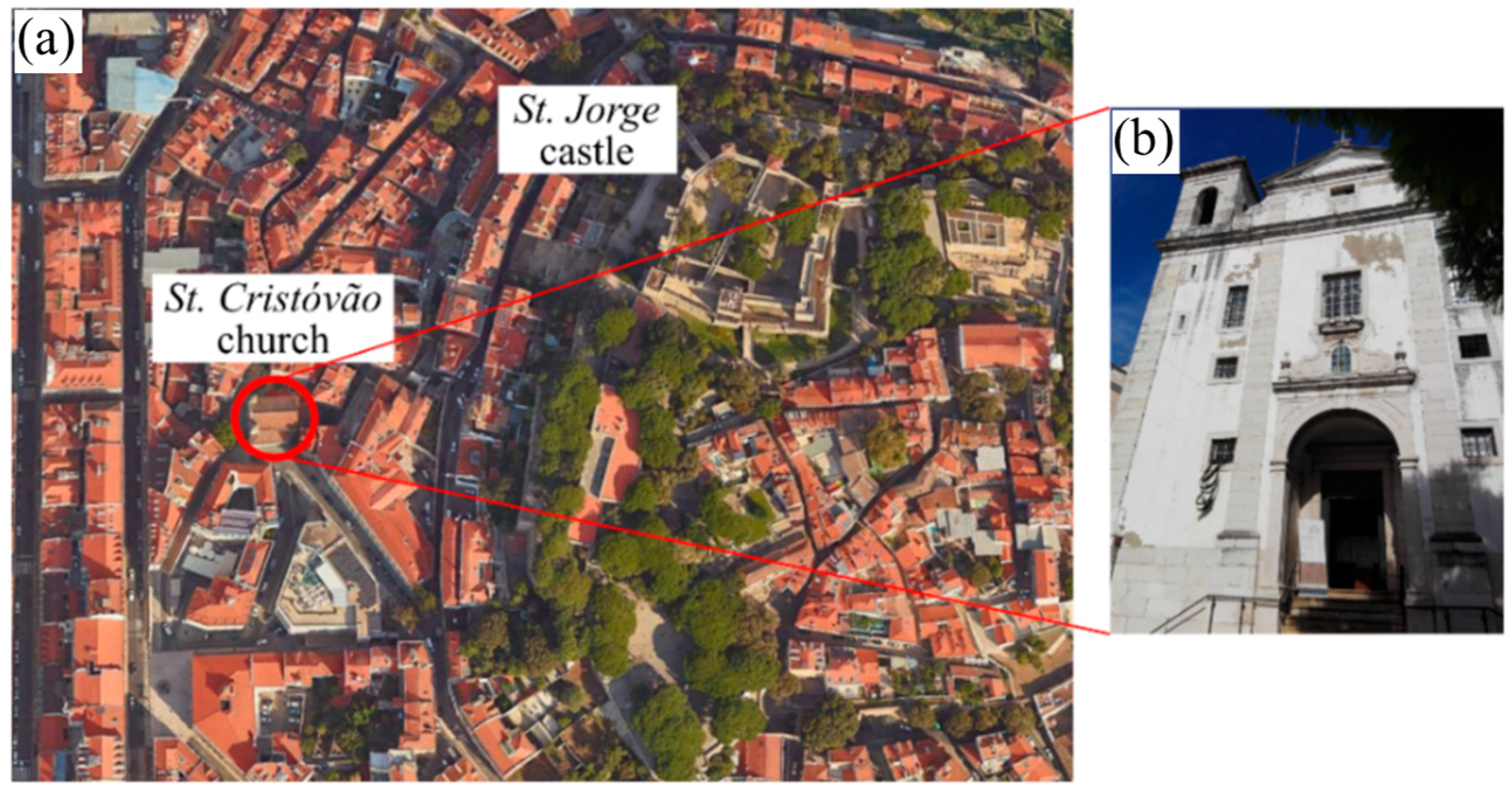
The simulations presented in this paper are based on a case study, i.e., St. Cristóvão church, which is a 13th-century church that is located in the vicinity of St. Jorge Castle in Lisbon (Figure 1). The church has thick, mortared limestone walls, single-glazed windows, and a ceramic tile roof, and it does not have any type of climate control system [17]. The church, which is naturally ventilated, has several compartments, with the largest ones being the nave, the mortuary, and the sacristy. Overall, the church has a volume of 5250 m3, and the window (45 m2) per wall area (800 m2) ratio is 0.056 [35]. St. Cristóvão church has a large variety of artifacts, among which sculptures and panel paintings [36].

Figure 1.
Location (a) and façade (b) of St. Cristóvão Church, Lisbon.
The church was subjected to a long-term monitoring campaign from November 2011 to August 2013 that used several sensors to later on determine the quality of the indoor climate in terms of artifacts conservation [17]. Subsequentially, the recorded data were used in the calibration process of computational models of the church [16,37]. The outdoor temperature and relative humidity in the vicinity of the church were monitored to build an outdoor weather file, which was then used to run the church models [16].
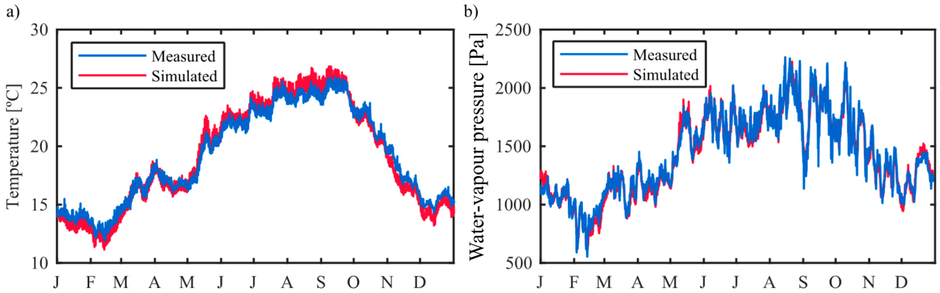
St. Cristóvão model was calibrated using four statistical indices, and the measured temperature (T) and water-vapor pressure (Pυ), namely [16]: coefficient of determination (R2—0.99 for T and 0.97 for Pυ), normalized mean bias error (NMBE—2.7% for T and 3.4% for Pυ), coefficient of variation of the root mean square error (CV(RMSE)—3.2% for T and 4.4% for Pυ), and goodness-of-fit (fit—84.8% for T and 81.7% for Pυ). Considering the values that exist in the models published in the literature and the limits that exist in the specifications/guidelines [38], the obtained values for the St. Cristóvão model are quite suitable, which validates this model [16]. The results of this validation can be seen in Figure 2, which presents the measured and simulated indoor temperature and water-vapor pressure for St. Cristóvão. A detailed explanation of the performed monitoring campaign in St. Cristóvão church can be found in Ref. [17], while Ref. [16] thoroughly describes the development and validation procedure of the whole-building hygrothermal model used in this study.

Figure 2.
Simulated and measured indoor temperature (a) and water-vapor pressure (b) variations for the St. Cristóvão model (adapted from Ref. [16]).
Several types of retrofit measures were tested individually (Table 1), i.e., installation of internal insulation thermal systems and application of an external thermal insulation system (to the exterior walls), replacement of the existing windows systems by more energy efficient ones, and installation of a thermal insulation system in the ceiling/roof [39]. The materials used are included in the WUFI database [8].

Table 1.
Overview of the tested retrofit measures.
2.3. Artifacts Decay Processes
Artifacts can be prone to three types of decay depending on the indoor conditions, i.e., biological, chemical, and/or mechanical decay. Each of these types of decay is assessed using a respective method that will be briefly described in this subchapter. More information concerning these topics can be found elsewhere [29].
Biological decay in materials will be assessed using the mold risk factor (MRF) [40], which will be calculated based on the isopleth method [41]. In order for mold to grow in organic materials, it is necessary that certain values of temperature and relative humidity are met, but it is also necessary that the substrate has the necessary nutrients for mold to grow [41]. For each timestep, the values of temperature and relative humidity are compared against the Lowest Isopleth for Mold (LIM) curve to determine if this value is overcome. In case LIM is overcome, then the spores become active fungi, and their respective time contribution is added to the overall mold risk factor (Ref. [41] shows how these time contributions are calculated). The spores became fully active fungi when MRF is 1.0 [40].
Chemical decay in materials will be assessed using the lifetime multiplier concept [42], more precisely, the equivalent lifetime multiplier concept. This latter concept manages to characterize the material’s respawn to chemical decay under a single value [35]. Materials such as paper (activation energy of 100 kJ/mol [29]) and varnish (activation energy of 70 kJ/mol [29]) are prone to this type of decay. The lifetime multiplier concept is based on the Arrhenius equation, and it determines the time spans that material remains usable when compared to standard conditions, i.e., 20 °C and 50% RH. The equivalent lifetime multiplier (eLM, -), which is the average of the reciprocal of the lifetime multiplier values for the analyzed time period [42], is calculated using the following equation:
where n is the number of data points in the selected period (-), RHi is the surface relative humidity at instant i (%), Ea is the activation energy (J/mol), R is the gas constant (8.314 J/Kmol), and Ti is the temperature at instant i (°C).
Mechanical decay is a crucial damaging process for hygroscopic materials, which is mainly governed by the variation of the relative humidity since it will cause the moisture content of these materials to vary. In turn, this moisture content variation will damage the materials due to the prompted shrink/swell cycles [29]. Moreover, if objects are composed by two or more hygroscopic materials, the damage can be heightened since they will have different characteristics and, therefore, they will respond differently to the indoor climate variations [29].
Four different models were used to assess the risk of mechanical decay, namely: furniture, the model developed by Bratasz et al. [43]; sculptures, the model developed by Jakiela et al. [44]; and panel paintings, which had to be assessed using two different models due to the different characteristics of its constituents. The base layer was assessed using the model developed by Mecklenburg et al. [45], and the pictorial layer was assessed using the model developed by Bratasz et al. [46]. Martens [29] adapted these four models so that they could be used based on the indoor conditions recorded by monitoring campaigns or the results obtained from computational models.
2.4. Selected Outdoor Climates and Developed Methodology to Build the Respective Weather Files
Seville has a temperate climate with relatively high temperatures during the summer and does not reach below zero temperatures during winter. It rains moderately all year round, but the more prominent rains occur during winter, and the rains are less frequent during summer. On the other hand, Oslo is a humid continental climate, in which the temperature reaches below zero values a great part of winter, and the rains are more prominent also during winter.
In terms of temperature and water-vapor pressure, the expected trend is similar for the two climates, i.e., there is a substantial increase across the 21st century with RCP 8.5, as expected, attaining higher values in the far future [34]. In terms of precipitation and global radiation, two opposite behaviors are expected to occur, which depend on the location. Precipitation is expected to decrease, and global radiation is expected to increase for the Mediterranean climate, while for Oslo, the opposite is expected to occur [34].
The weather files used in this paper were created following the methodology described in Coelho and Henriques [39]. The past and future weather files were created using 30 years’ worth of data, as recommended by the World Meteorological Organization [47]. The meteorological data were downloaded from the CORDEX database [48]. The weather files were built using the methodology described in EN 15927-4 [49]. The global radiation was subdivided into its direct and diffuse fractions using the Skartveit and Olseth model [50], which is one of the most reliable models to perform this subdivision [51]. More information concerning the topic can be found in Ref. [34].
2.5. Time-Saving Measures
In order to proficiently perform the proposed simulations, a new methodology to reduce the overall simulation time of whole-building hygrothermal studies was developed. Simulation studies, which already have the computational model calibrated, can be divided into four steps (Figure 3): (1) setting up the simulations inputs; (2) performing the simulations; (3) processing the obtained results in figures or tables; (4) assessing the results and writing conclusions.

Figure 3.
Scheme of the four stages of simulation studies.
The duration of each of these steps will greatly depend on the aim of the performed study. The purpose of this procedure is to minimize the time taken to perform each of the first three stages:
Step 1 (Simulation setup): The time spent on this step can be reduced drastically by automatically inserting the inputs, for example, using external software, such as MATLAB or OCTAVE. In WUFI®Plus, the users can save the project as an mwp file (traditional way of saving files in WUFI®Plus) or as an xml file. This latter type of file allows one to change its parameters, such as the thickness of a material or the location of the outdoor climate weather file, by resorting, for example, to a code that is developed for that purpose [34]. This step has a very substantial time-saving effect on simulation studies that are subdivided into several computers. In addition, this step also decreases the possibility of human error since the inputs are automatically introduced, thus eradicating monotonous tasks.
Step 2 (Simulation run): The time spent on this step can be reduced by performing the simulations resorting to batch mode, which allows running the simulations sequentially, and by dividing the simulations through several computers. This measure can lead to an increase in the individual simulation time if the computers are not modern, but it ultimately decreases the overall simulation time. For example, Coelho et al. [28] initially used a computer equipped with an Intel(R) Core(TM) i5-8500 CPU @ 3.00 GHz and 16 GB of RAM to perform the hygrothermal simulations (henceforth known as PC#1), which took between 1 h and 1 h 30 min to run depending on the outdoor climate. Alternatively, they used a set of 20 computers equipped with an Intel(R) Core(TM) i5-650 CPU @ 3.20 GHz and 4 GB of RAM (henceforth known as PC#2) to run the same simulations and took at least 3 h. However, the overall simulation time, i.e., the sum of all the individual simulation times, is much lower in the 20 PC#2 than in the PC#1. Taking into account the previously mentioned simulations run time for PC#1, and if we chose to run, for example, 20 simulations in PC#1, this would mean that the overall simulation time would take between 20 and 30 h, depending on the outdoor climate. On the other hand, if we run the same number of simulations but divide them between the 20 PC#2, the overall simulation time is around 3 h, which means a reduction of 85–90% of the overall simulation time.
Step 3 (Result processing): The time spent on this step can be substantially decreased if instead of using the traditional excel spreadsheets, a software that is aimed at numerical calculation is used, such as, for example, MATLAB or OCTAVE. Evidently, the users will spend time developing the code for the analysis that they aim to perform. However, if the code is developed taking into consideration that it might be adapted to assess a larger number of simulations or a large number of inputs in the future, the time it takes to make this change is compensated when compared to performing the same task in Excel spreadsheets. This step gains importance with the growing complexity of the analysis and decreases the time taken to perform the same analysis for other sets of simulations very considerably when compared to Excel spreadsheets.
Alternative to using a set of several computers, as mentioned previously, it is possible to use a single computer, but it has to be a rather powerful one to compensate for the performance of the individual computers. With WUFI®Plus, which has the drawback of only performing the simulations sequentially, the computer has to be powerful enough to at least perform each simulation in 9 min in order to compensate for the performance of the set of computers used by Coelho et al. [28]. However, these powerful computers are considerably more expensive than the typical office/personal computers (e.g., [52]).
A task that can also be greatly time-consuming is the insertion of the building geometry into the simulation software. Fortunately, WUFI®Plus has three different options to introduce the geometry, namely: 3-D editor, SketchUp import, and gbXML Import. The 3-D editor consists of inputting the vertices of each surface manually and then uniting them to build each surface. This is a very time-consuming way of introducing geometry and gives way to inconsistencies for more complex geometries. On the other hand, the SketchUp import and gbXML import are much more efficient ways of introducing the geometry since the case study is designed in software that is aimed for that purpose. The gbXML import can have key importance for projects of new buildings since it allows the use of building geometries developed in Revit by performing the proper conversion [8].
3. Results and Discussion
This section is divided into two subsections due to the paper’s goals. Section 3.1 analyzes the potential of the selected passive retrofit measures to mitigate the effects of climate change in the decay of artifacts, and Section 3.2 shows the benefits of the methodology described in Section 2.5 by presenting the respective time savings for the study partially presented in Section 3.1 and complemented by the studies discussed in Refs [34,39].
Moreover, Section 3.1 is divided into two parts: (1) where several indoor climates are assessed in terms of risk of biological decay (Figure 4a,b), chemical decay (Figure 5a,b), and mechanical decay (Figure 6a–d); and (2) recommended thicknesses range for the tested retrofit measures for walls, as well as ceilings/roofs for both Seville and Oslo. These figures are an example of an analysis fully presented in Ref. [34]. Figure 4 concerns retrofit measure W4, Figure 5 concerns measure W1, and Figure 6 concerns measure W4. The minimum recommended thickness corresponds to the case in which it is worth applying, depending on the analyzed parameter, when compared with the case study without any retrofit measure (Table 2).

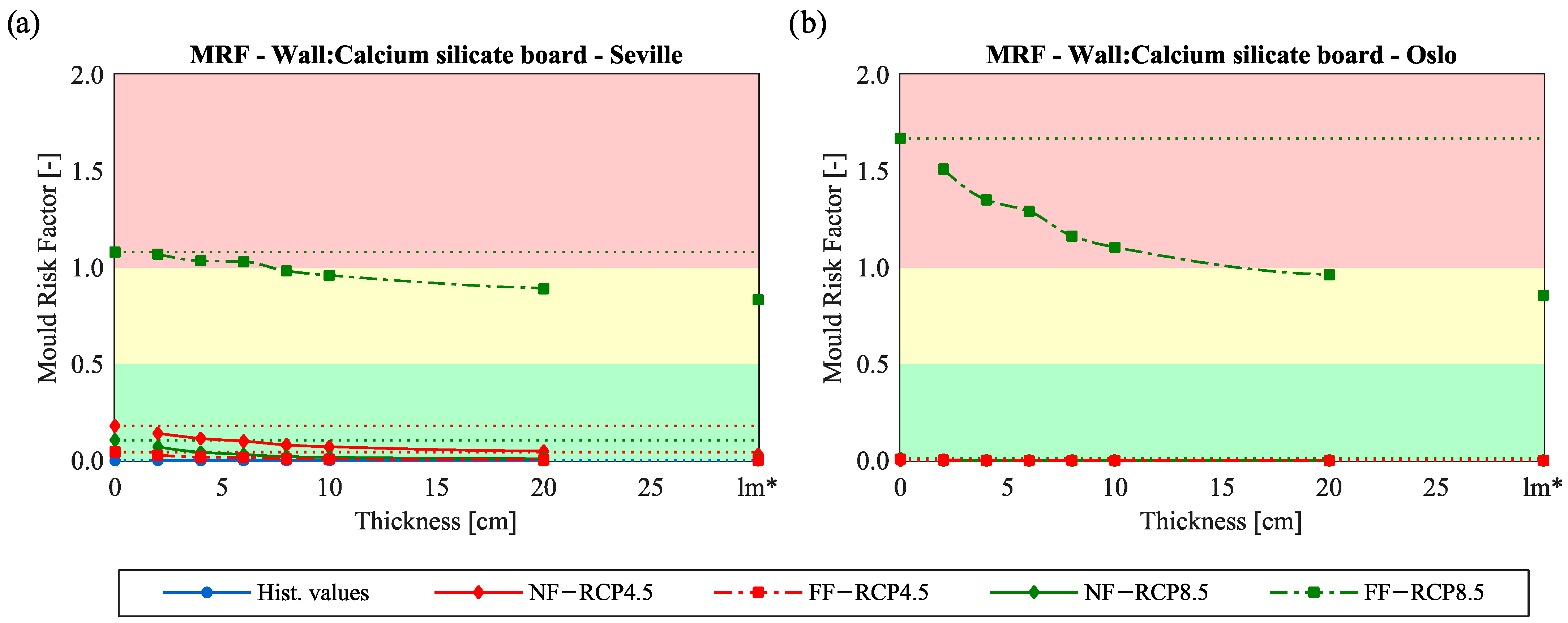
Figure 4.
Biological decay assessment (MRF) for the case study with calcium silicate board for Seville (a) and Oslo (b). This figure shows the results for historical, near-future, and far-future time frames for the case study with a wall retrofit measure and for the case without retrofits (dotted lines). lm* is an additional “virtual” thickness that corresponds to a 30 cm layer.

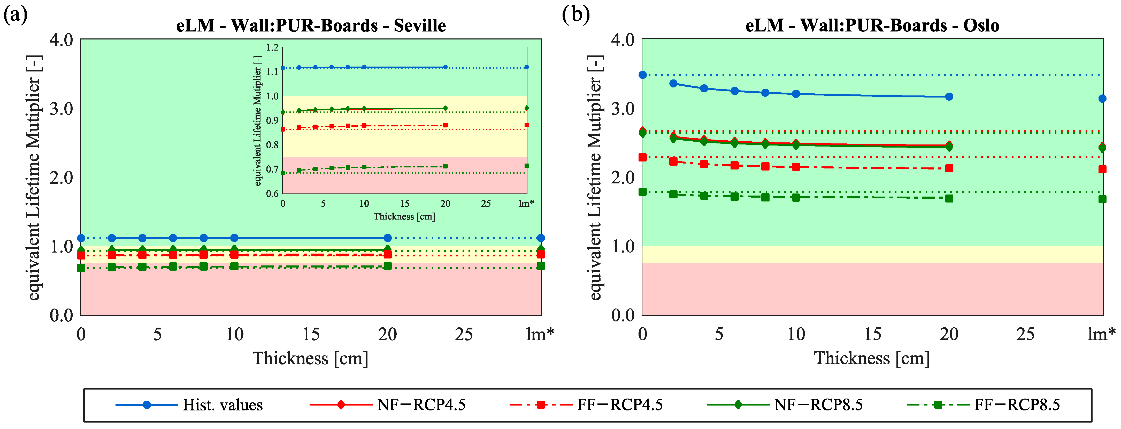
Figure 5.
Chemical decay assessment (eLM) for the case study with PUR boards for Seville (a) and Oslo (b). This figure shows the results for historical, near-future, and far-future time frames for the case study with a wall retrofit measure and for the case without retrofits (dotted lines). lm* is an additional “virtual” thickness that corresponds to a 30 cm layer.

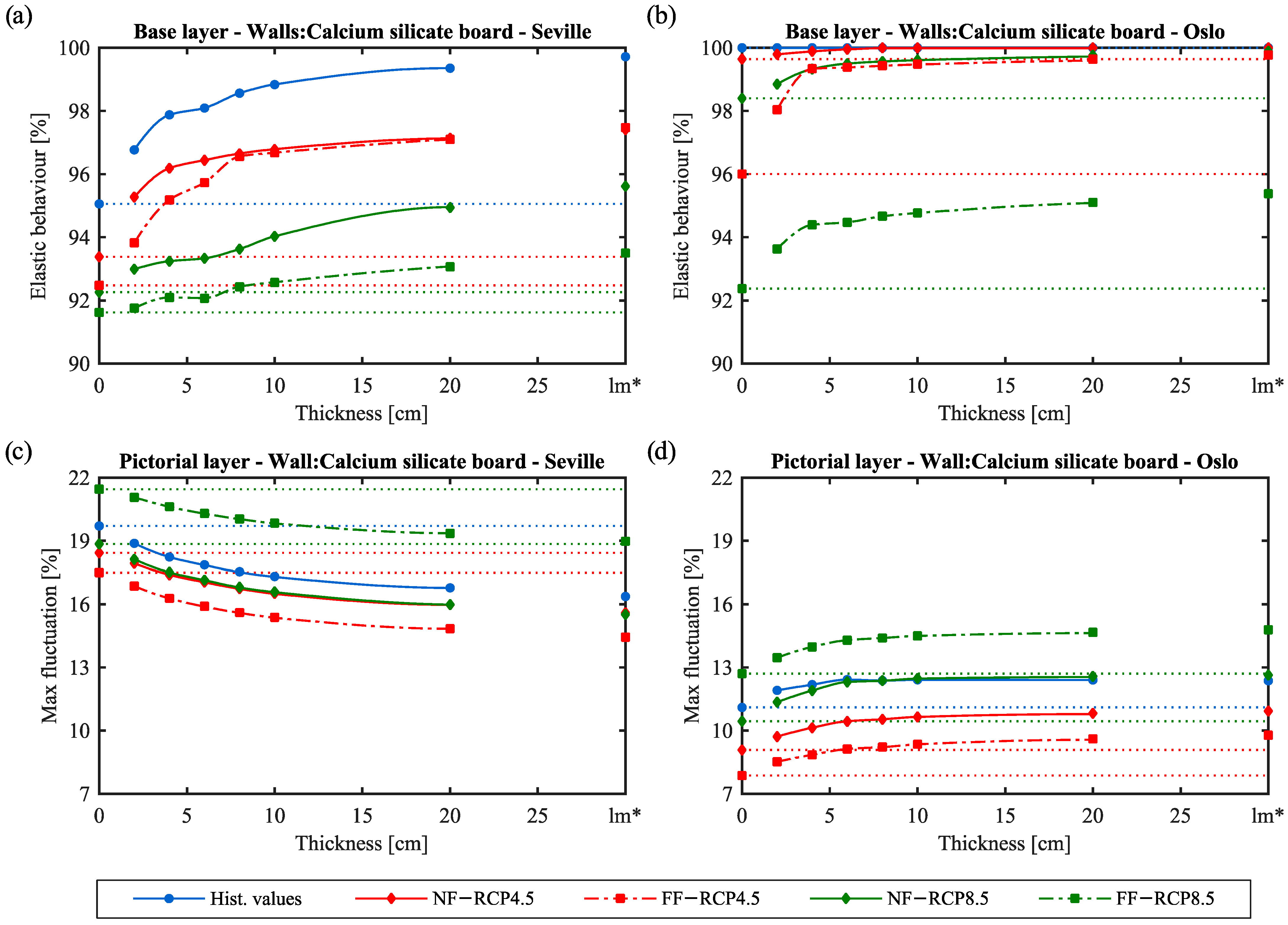
Figure 6.
Mechanical decay assessment for the base layer of panel paintings for the case study with calcium silicate board for Seville (a) and Oslo (b); and mechanical decay assessment for the pictorial layer of panel paintings for the case study with calcium silicate board for Seville (c) and Oslo (d). This figure shows the results for historical, near-future, and far-future time frames for the case study with a wall retrofit measure and for the case without retrofits (dotted lines). lm* is an additional “virtual” thickness that corresponds to a 30 cm layer.
Table 2.
Thickness range (cm) that outperforms the case study without any retrofit measure (WR) for Seville and Oslo for future conditions: RCP 4.5 and RCP 8.5.
Overall, this study includes two different climates: Seville (Spain) and Oslo (Norway), two IPCC scenarios: RCP 4.5 and RCP 8.5, and two future time frames: near future (NF) and far future (FF). Additionally, a historical climate is also included in the study that acts as a reference for the performed assessments (i.e., “Hist. values” in Figure 4, Figure 5, and Figure 6). The thicknesses of the tested thermal layers for walls range between 2 and 20 cm. An additional “virtual” thickness, named lm*, which corresponds to a 30 cm layer, was included in Figure 4, Figure 5, and Figure 6 to show the tendency that the performed assessments would have for higher thicknesses [39]. These figures have a color code that follows the limits proposed by Silva [53]: (1) MRF < 0.5 (green), 0.5 < MRF < 1 (yellow), and MRF > 1 (red); and (2) eLM > 1 (green); 0.75 ≤ eLM < 1 (yellow) and eLM < 0.75 (red).
3.1. Detailed Analysis of a Set of Retrofit Measures for Historic Buildings That House Artifacts: Seville, Spain vs. Oslo, Norway
3.1.1. Biological Decay
The tested retrofit measures reduce the increasing risk of biological attacks caused by climate change in Seville, which is more pronounced for RCP 8.5 in the far future (Figure 4a). On the other hand, Oslo is not prone to biological decay (Figure 4b) due to its lower indoor temperature and relative humidity when compared to the Mediterranean climate [12]. The only exception to this behavior occurs in the far future and if the world evolves according to scenario RCP 8.5 (Figure 4b). If this scenario prevails, then MRF amounts to values well above 1.0 in Oslo, which is a risk for the preservation of the artifacts. For these conditions, the MRF is 1.7 for the case without retrofit measure.
Nonetheless, in both cases, i.e., Seville and Oslo in the far future for RCP 8.5, the efficiency of the application of the wall retrofit measures (Figure 4a,b, respectively) can be observed since the MRF decreases considerably and attains values lower than 1.0 for a wall calcium silicate board system thicker than 7.3 cm for Seville and 15.7 cm for Oslo. In addition, the inferior limits upon which it is worth applying the thermal insulation systems vary according to the type of insulation layer and climate change scenario, as will be shown and discussed further ahead (Table 2).
In terms of the ceilings and roofs, the worrying situation is the far future for scenario RCP 8.5 [34], in which the MRF values are well above the 0.5 safety limit. However, the application of the retrofitted measures decreases this risk since it is responsible for lowering the MRF. This reduction is only significant for the first tested thickness for Seville, which leads to the belief that this occurs mainly due to the air tightening of the roof that is caused by the application of the insulation system. The exception is the mineral wool retrofit, which is only worth installing from a certain thickness onwards (Table 2). Finally, the replacement of the window system does not affect both climates substantially because high thermal inertia buildings, such as the case study, typically have low wall/window ratios [35].
3.1.2. Chemical Decay
Climate change is responsible for an increase in the risk of chemical decay in artifacts for both analyzed climates (Figure 5a for Seville and Figure 5b for Oslo). For instance, the eLM for Seville in the reference climate is 1.12, but when climate change is considered, either RCP 4.5 or RCP 8.5 scenarios, the situation worsens considerably, especially for RCP 8.5 in the far future, in which the eLM is 0.68, i.e., a decrease of 39% when compared with the reference climate value. Nevertheless, it is also visible that the application of the retrofit measures increases the eLM for Seville (Figure 5a), thus tackling the negative effects of climate change by reducing the risk of chemical decay.
The application of the retrofit measures in Seville will lead to an increase in the indoor temperature and relative humidity during winter and autumn and a decrease in the indoor temperature during summer and spring. While the first behavior will result in a decrease in the LM, the second behavior will increase the LM. This behavior gains importance with climate change since the decrease in temperature during these two seasons is more prominent, which will lead to superseding the first behavior impact, thus leading to the increase in the eLM. These behaviors occur for all tested wall retrofit measures [34]. Note that these retrofit measures were tested individually and, therefore, can have a greater mitigation potential if they are properly combined [54,55].
On the other hand, the application of the retrofit measures for Oslo leads to an increase in the risk of chemical decay since they are responsible for decreasing the eLM (Figure 5b). However, since the initial values are quite high (i.e., 3.49 for the PUR boards retrofit for the reference climate) due to the lower indoor temperature and relative humidity, and they are still within the safe range (i.e., eLM above 1.0 [53]), then the retrofit measures can still be applied if they aim to mitigate other decay mechanisms. In terms of ceilings and roofs, the results are not substantial for both climates [34]. Once again, the replacement of the window system does not affect both indoor climates substantially [34].
3.1.3. Mechanical Decay
Climate change is responsible for the increase in the risk of mechanical decay for the base layer of panel paintings for both Seville (Figure 6a) and Oslo (Figure 6b), although it is more substantial for the first climate. For instance, for the case study without retrofit measures, 95.1% of the year in Seville is under elastic behavior (Figure 6a), while for the worst-case scenario—i.e., RCP 8.5 in the far future—this value decreases to 91.6% (Figure 6a). However, by applying the retrofit measures, this risk decreases substantially, e.g., the values for the reference climate increases to 99.4% for an insulation system composed of 20 cm of calcium silicate board. For the same conditions, the values are 100% and 92.4% for Oslo, but for this climate, the retrofit measures are even capable of reaching the 100%-value for relatively thin wall insulation systems, which reinforces the notion that climate change has a more substantial effect in Seville.
In terms of the pictorial layer (of the panel paintings), it is visible that the application of the retrofit measures will decrease the risk of mechanical decay in Seville since the maximum fluctuation will decrease substantially (Figure 6c). For example, for the reference climate without any retrofit measures, the maximum fluctuation is 19.7%, while for a 20 cm wall calcium silicate board retrofit, it is 16.8%. For the climate of Seville, most of the selected time periods that correspond to climate change scenarios have lower values than those of the reference climate, the only exception being the far future for RCP 8.5, which corresponds to the most demanding scenario [23]. These behaviors are also visible for the remaining wall retrofit measures and also for the other retrofit measures, such as the ceiling and roof retrofit and window replacement, but to a much lower extent [34].
On the other hand, Olso has a different behavior, in which the application of the retrofit measures increases the maximum fluctuation, although only the RCP 8.5 far future is above the reference climate (Figure 6d). Nonetheless, these values are mostly below the 14% safety limit [56], which means that these retrofit measures can be applied to prevent other types of decay from occurring or for other reasons (e.g., improve indoor thermal comfort [54]), without putting the pictorial panels of the panel paintings in jeopardy. The previously described behavior is also visible for the remaining tested retrofit measures but to a lower extent for the non-wall retrofit measures [34].
The tested retrofit measures for the ceilings and roofs also decrease the risk of mechanical decay, but this reduction is only significant for the first tested thickness, which once again leads to the belief that this is due to the air tightening of the roof. The replacement of the window system does not affect both indoor climates substantially [34], because high thermal inertia buildings typically have low wall/window ratios [35].
No substantial differences caused by climate change and the application of the retrofit measures in terms of mechanical decay assessment concerning the furniture are detected [34], which means that the tested retrofit measures can be applied to mitigate other decay mechanisms without compromising the mechanical integrity of furniture artifacts. Still, climate change will slightly increase the risk of mechanical decay for sculptures [34]. Normally, the whole year corresponds to an elastic behavior (i.e., 100%), but climate change will be responsible for decreases below 2%. Nonetheless, the application of retrofit measures will counteract this behavior [34].
3.1.4. Recommended Thicknesses Ranges for Wall Assemblies and Ceilings/Roofs for Seville and Oslo
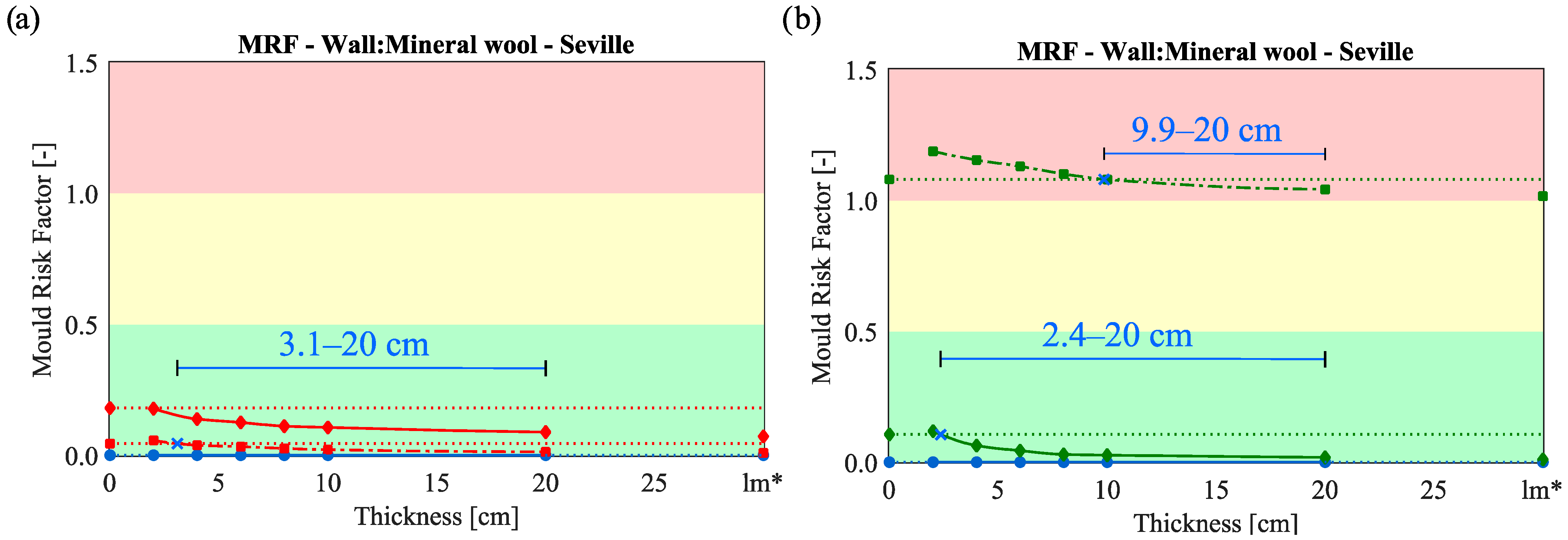
The idea behind this analysis is to find the minimum thickness that is worth applying as a retrofit in the near future (green solid line—Figure 7a—or red solid line—Figure 7b) and in the far future (green dash-dotted line—Figure 7a—or red dash-dotted line—Figure 7b). This objective is achieved by comparing the results against the value for the case that does not have any retrofit measure, i.e., dotted red or green lines.

Figure 7.
Recommended thickness ranges for mineral wool retrofit if the world evolves as described in RCP 4.5 (a), in the near future (NF) and far future (FF) for MRF, or as described in RCP 8.5 (b), in the near future (NF) and far future (FF) for MRF. lm* is an additional “virtual” thickness that corresponds to a 30 cm layer.
As can be seen in Figure 7 for the MRF analysis, this results in a thickness range that differs according to the time interval, as well as the climate change scenario. This is understandable since the indoor conditions will also differ accordingly [34]. For example, in Figure 7b, the recommended thicknesses for the near-future range are between 2.4 and 20 cm, while the recommended thicknesses for the far-future ranges are between 9.9 and 20 cm for RCP 4.5.
Hence, the recommended thickness ranges that appear in Table 2 are the intersection between ranges for both time frames, i.e., 2.4–20 cm for NF and 9.9–20 cm for FF, which leads to the 10–20 cm range for the mineral wool retrofit (W2) for the MRF parameter in the RCP 8.5 scenario. It is visible that RCP 8.5 is more demanding since shorter thickness ranges are recommended and that Oslo’s climate is less demanding when compared to Seville’s climate. The thicknesses are rounded up to unit values since these types of insulation layers are normally commercialized in centimeters, and, in this way, they are within the recommended range.
Table 2 allows us to determine from which thickness onward is worth applying the retrofit measures so that the case study can withstand future conditions in accordance with the parameter that is being analyzed. However, it is also possible to obtain a more compressive thickness range if more than one parameter is taken into account (e.g., if the MRF and the eLM are both considered for the perlite board retrofit (W2) for Seville in RCP 4.5, this means a recommended range of 11–20 cm), but this will also probably lead to a more stringent thickness range [34].
3.2. Application of the Time-Saving Methodology
The study shown in the previous section, which is complemented by studies presented in Refs [34,39], corresponds to the thorough analysis of the application of passive retrofit measures in historic buildings that house artifacts while considering climate change. The effect of each of the selected passive retrofit measures was assessed in terms of artifacts’ conservation metrics to see if they could mitigate the changes caused by climate change. In total, the study includes five climates and two of the newest IPCC scenarios: RCP 4.5 and RCP 8.5.
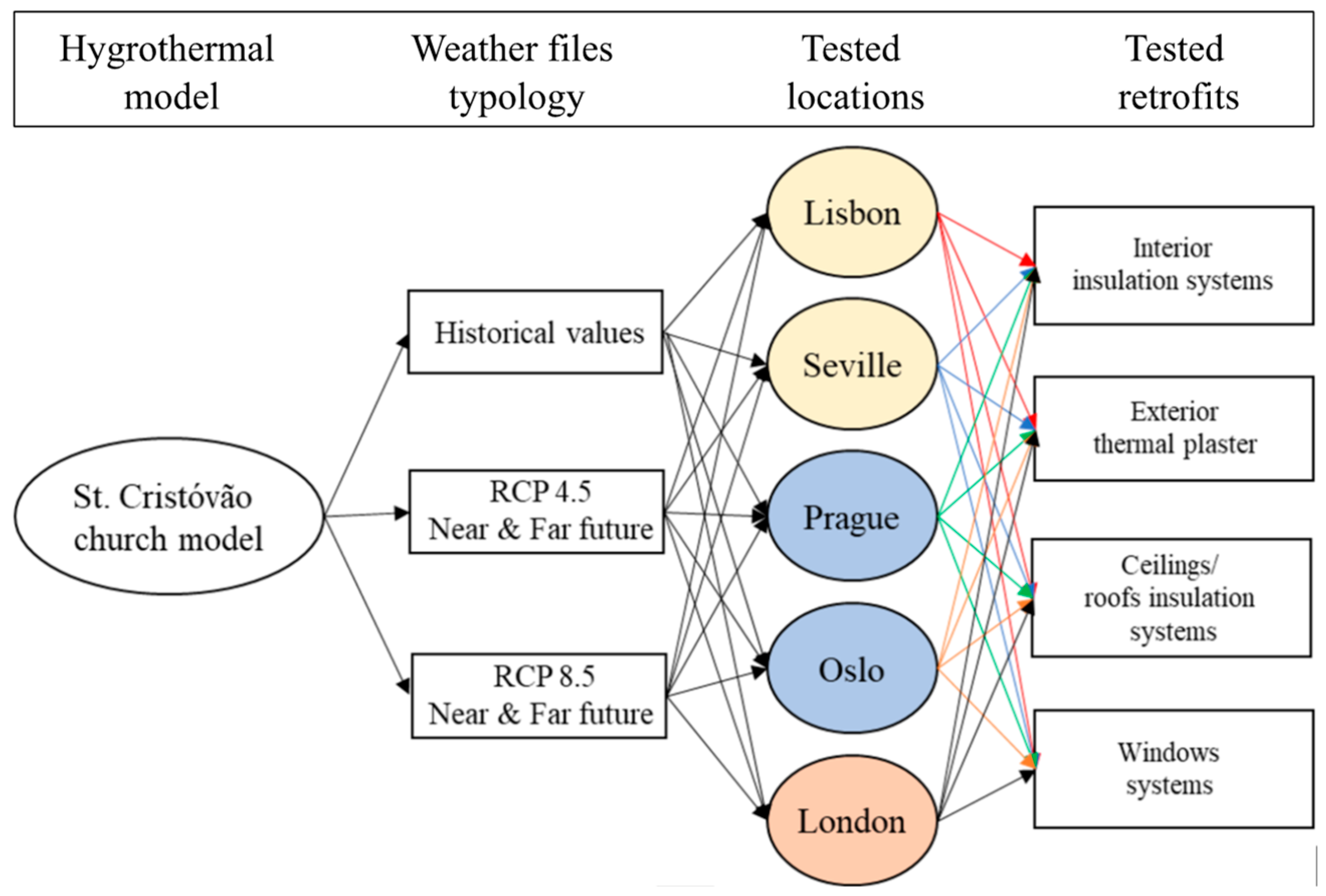
Overall, 1350 simulations were run in WUFI®Plus to perform this analysis (Figure 8), which would take ca. 1485 h to run in PC#1, i.e., almost 62 days of continuous simulation. Instead, the simulations were subdivided by 20 PC#2, which resulted in a decrease of 62% of the simulation run time since it dropped from 1485 to 567 h.

Figure 8.
Scheme of the developed simulations in Ref. [34] to assess the performance of four types of retrofit measures in historic buildings that house artifacts for five climates and two IPCC scenarios in the near future and far future in terms of artifacts conservation metrics.
For assessing the effects of the selected passive retrofit measures, the results-processing stage is important because the numerical processes included in this example are more complex (e.g., Figure A1 for assessing the biological decay) than simply sum values (e.g., Figure A2 [28]). The indoor climate was assessed using three different analyses [29]: i.e., biological decay using the isopleth method, chemical decay using the equivalent lifetime concept, and mechanical decay in which the method varies according to the material. Secondly, in this example, the obtained values are compared against sets of values for each timestep, which takes much more time to perform.
Instead of taking ca. 34 h to process the obtained data using the traditional methodology, the data were assessed and presented in the form of the figures shown in Section 3.1 under 17 h using MATLAB. The benefits of using this type of software are more obvious when performing similar analyses in which the necessary adaptations will only take a few minutes to perform, whereas, in the traditional methodology, this could take up to several hours, depending on the complexity of the analysis. In addition, the use of MATLAB has the advantage of performing the work independently from the user, contrary to the traditional methodology, in which the updates have to be performed manually. This means that while MATLAB is assessing data, the user can develop other tasks.
Another problem that gained emphasis due to the subdivision of the simulations among several computers was the time taken to set up the simulations to run. This procedure is normally performed manually, which takes a considerable amount of time to perform, and it will depend on the number of simulations that are assigned to each computer. For instance, if each of the 20 PC#2 were assigned 20 simulations to run, then the time spent to set up all the 400 simulations would be almost 7 h. It took around 20 min to set each computer in Ref. [34] since this included the inputting of the necessary data for the model to run properly, as well as checking if the inputs were well introduced in the model.
In order to decrease the amount of time taken by this procedure, an original code that automatically sets the inputs in the WUFI model was written in XML language. The WUFI model is saved as an xml file instead of the typical mwp file, and then it is changed using either MATLAB or OCTAVE. This procedure allows for saving a large amount of time when performing changes in existing simulations and facilitates the process of creating new simulations considerably, which is fundamental for large-sized hygrothermal simulation studies. Furthermore, this development decreases the possibility of human error since the software user no longer has to perform the same monotonous procedure for a large number of simulations.
Instead of taking 20 min to set up each computer, the simulations were set up in 2.5 s. The time it would take to set up the 400 simulations will decrease from ca. 7 h to ca. 50 s. Overall, this means that the time it would take to set up the 1350 simulations manually would be ca. 23 h. Since the XML code cuts this time to 3 min, the simulation’s overall run and setup time would drop 62%, i.e., from 1542 to 584 h. The larger the number of simulations included in the performed analysis is, the more effective becomes this time-saving procedure.
In order to show the advantages of the methodology presented herein more straightforwardly, the time savings discussed throughout this section of the paper are summarized in Table 3. Based on the values presented in this table, it is visible that setting up the simulations becomes negligible in terms of time consumption. A task that takes almost a day to perform manually only takes at most 3 min to perform using software such as MATLAB.
Table 3.
Time savings achieved using the developed methodology for the examples presented in Section 3.2.
The data processing becomes almost non-time-consuming, although the extent of the time savings will depend on the analysis that has been performed [34]. By replacing the traditional way of processing the data for software such as MATLAB, the data processing in Section 3.2 drops from taking 34 hours to complete to only ca. 17 hours (i.e., a 51% drop). The data processing in this type of software is independent once it starts, so the time it takes to perform this task can be used to develop other tasks. Finally, the simulation run time also decreases substantially, i.e., 62%, but this decrease will greatly depend on the aims of the analysis, more specifically, in terms of outdoor climates [34].
4. Conclusions
In order to safeguard artifacts housed in historic buildings from the effects that climate change will have on the indoor climate of these types of buildings, several passive retrofit measures were tested in this study. To achieve this goal, the following tools were used: (1) a calibrated whole-building hygrothermal model of a high thermal inertia building; (2) future weather files: RCP 4.5 and RCP 8.5; and (3) decay assessment models: biological, chemical, and mechanical. Moreover, to determine how the mitigation potential of the retrofit measures would vary in accordance with the location, two different types of climates were tested: a Mediterranean climate (Seville, Spain) and a humid continental climate (Oslo, Norway). In addition, insulation layer thicknesses range for the tested wall assemblies and ceilings/roofs are also recommended. Lastly, the benefits of the therein methodology that aims to reduce the overall simulation time of whole-building hygrothermal studies are also presented in terms of time savings.
Overall, it was visible that the retrofit measures can mitigate, to a certain extent, the effects that climate change will have in terms of the increase in the risk of mechanical, biological, and chemical decay. It was also shown that the passive retrofit potential would vary in accordance with the climate. In addition, it is the authors’ belief that their mitigation potential can even be heightened if they are properly combined (e.g., using multi-objective optimization). In accordance with the building type and use, but also the constitution of the building assemblies and ventilation rates, the outdoor climate, and eventually the climate change, can have a very significant influence on the indoor climate and, consequently, on the preservation of historical artifacts. In contrast, if the artifacts are kept in more recent buildings, which were built for the purpose of safekeeping artifacts and, due to today’s regulations in the construction sector, are more airtight, then the artifacts will be less prone to the attacks caused by the outdoor climate. Finally, it is safe to assume that the influence of the outdoor climate on the preservation metrics is largely dependent on the building specifications.
The tested retrofit measures reduce the increased risk of biological decay caused by climate change in Seville and Oslo, especially for RCP 8.5 in the far future. For example, the mold risk factor (MRF) decreases considerably and leaves the risk region for the preservation of the artifacts (i.e., values higher than 1.0) for a wall calcium silicate board system thicker than 7.3 cm for Seville and 15.7 cm for Oslo.
Climate change is also responsible for an increase in the risk of chemical decay since the equivalent lifetime multiplier (eLM) decreases considerably. For example, the eLM is 0.68 for Seville in the far future for RCP 8.5, i.e., a decrease of 39% when compared with the reference climate value (1.12). However, the tested retrofit measures manage to mitigate this increase to a certain extent. Due to the climate particularities, chemical decay-susceptible artifacts are unaffected by this type of decay in Oslo. In truth, climate change is responsible for the decrease in the eLM in Oslo, but as the values are quite high (e.g., 3.49 for the PUR boards retrofit for the reference climate), they do not reach the danger region, i.e., eLM below 1.0, for the analyzed RCP scenarios and time frames.
Climate change is also responsible for the increase in the risk of mechanical decay for the base layer of panel paintings for both analyzed climates. However, the retrofit measures manage to mitigate this occurrence considerably. For instance, the time the reference indoor climate for Seville is under elastic behavior increases from 95.1% to 99.4% with the application of a 20 cm of calcium silicate board insulation system. For Oslo, the application of the retrofit measures even enables the indoor climate to reach the 100%-limit in some of the analyzed scenarios and time frames.
In terms of the pictorial layer, the tested retrofit measures mitigate the effects of climate change in Seville for most of the analyzed cases, with the exception being the far future for RCP 8.5. On the other hand, the retrofit measures are responsible for increasing the maximum fluctuation, i.e., they are responsible for the worsening of the preservation conditions, but most of the analyzed cases are below the safety limit, with once again the exception being the RCP 8.5 far future. In contrast, climate change does not endanger furniture, nor does it significantly endanger sculptures.
Finally, a table with recommended thickness ranges that withstand future conditions for the parameter that is being analyzed is presented for wall assemblies and ceilings/roofs for both Seville and Oslo. This goal is achieved by comparing the results of the cases with retrofits against the values for the case that does not have any retrofit measure. This analysis enables us to choose an efficient retrofit measure for a specific case in which the indoor conditions are better than the case without retrofits. Ultimately, it was shown that in some cases, the application of a given retrofit measure is not recommended for a specific goal or that it is only worth applying it from a certain thickness onward.
In addition, this paper presents several strategies that aim to reduce the amount of time needed to perform large-sized hygrothermal simulation studies. All proposed strategies were organized in a methodology that makes this type of study more time efficient. This will allow the use of powerful tools, such as simulation software, to optimize buildings more frequently and straightforwardly. This methodology has been applied in several cases, which are briefly presented in this paper, and the amount of time saved by following this methodology is quite substantial.
The use of this methodology leads to substantial time savings at the several steps that incorporate the typical building simulation studies. By using MATLAB in the simulation setup, a task that would take ca. 23 h to perform manually only takes 3 min to perform, i.e., a time saving of almost 100%. Secondly, by dividing the simulations by 20 PCs, the overall simulation time decreased by 62%. This decrease has a key importance since it corresponds to the task that conditions this type of study because it is the one that takes longer to complete. Lastly, the data processing using MATLAB also has a substantial time reduction of ca. 51%, i.e., transforming a task that would take hours to complete into a task that can be performed in a matter of seconds. This task duration is greatly dependent on the complexity of the performed analysis. However, since it performs independently from the user, the drawback of its longer duration associated with more complex analysis is somehow lessened.
In addition, the automatic insertion of inputs in WUFI®Plus is a key advantage in simulation studies since it enables the development of an algorithm that updates the model’s inputs according to the model’s corresponding outputs until the termination criteria set by the authors are met. This procedure can have numerous applications, such as the development of a setpoint strategy for the HVAC system that adapts according to the number of people inside the building and their consequent effect on the conservation of artifacts.
Author Contributions
Conceptualization, G.B.A.C., V.P.d.F. and F.M.A.H.; Formal analysis, G.B.A.C.; Investigation, G.B.A.C.; Methodology, G.B.A.C., V.P.d.F. and F.M.A.H.; Software, G.B.A.C.; Validation, V.P.d.F., F.M.A.H. and H.E.S.; Visualization, G.B.A.C.; Writing—original draft, G.B.A.C.; Writing—review and editing, V.P.d.F., F.M.A.H. and H.E.S. All authors have read and agreed to the published version of the manuscript.
Funding
The first author acknowledges the FCT—Fundação para Ciência e a Tecnologia—for the financial support through the Ph.D. scholarship PD/BD/127844/2016. This work was financially supported by: UID/ECI/04708/2019- CONSTRUCT—Instituto de I&D em Estruturas e Construções funded by national funds through the FCT/MCTES (PIDDAC). The APC was funded by open access funds from Oslo Metropolitan University (OsloMet).
Institutional Review Board Statement
Not applicable.
Informed Consent Statement
Not applicable.
Data Availability Statement
Data will be made available on request.
Conflicts of Interest
The authors declare no conflict of interest. The funders had no role in the design of the study; in the collection, analyses, or interpretation of data; in the writing of the manuscript; or in the decision to publish the results.
Appendix

Figure A1.
Procedure for assessing the biological decay developed in MATLAB.
Figure A1.
Procedure for assessing the biological decay developed in MATLAB.
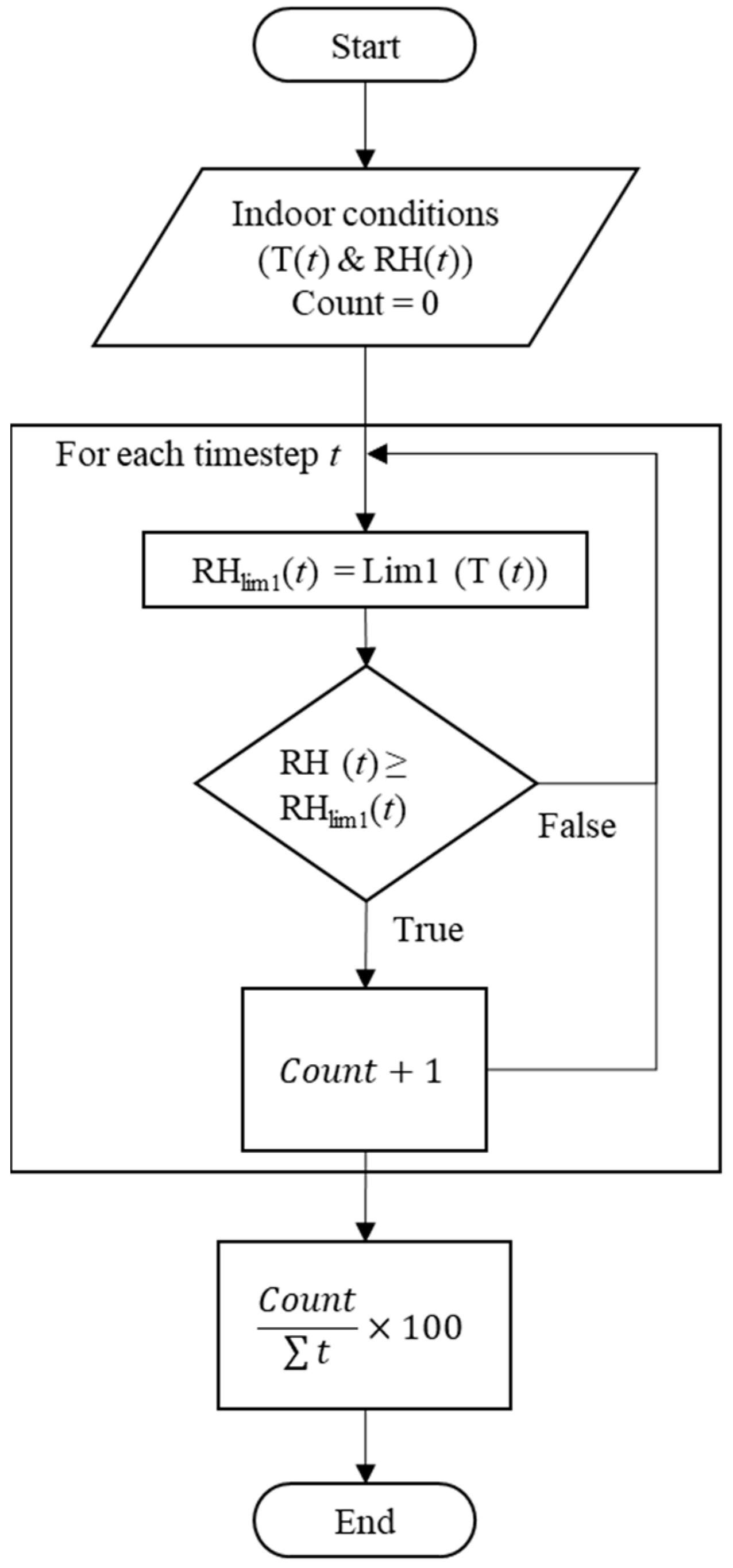

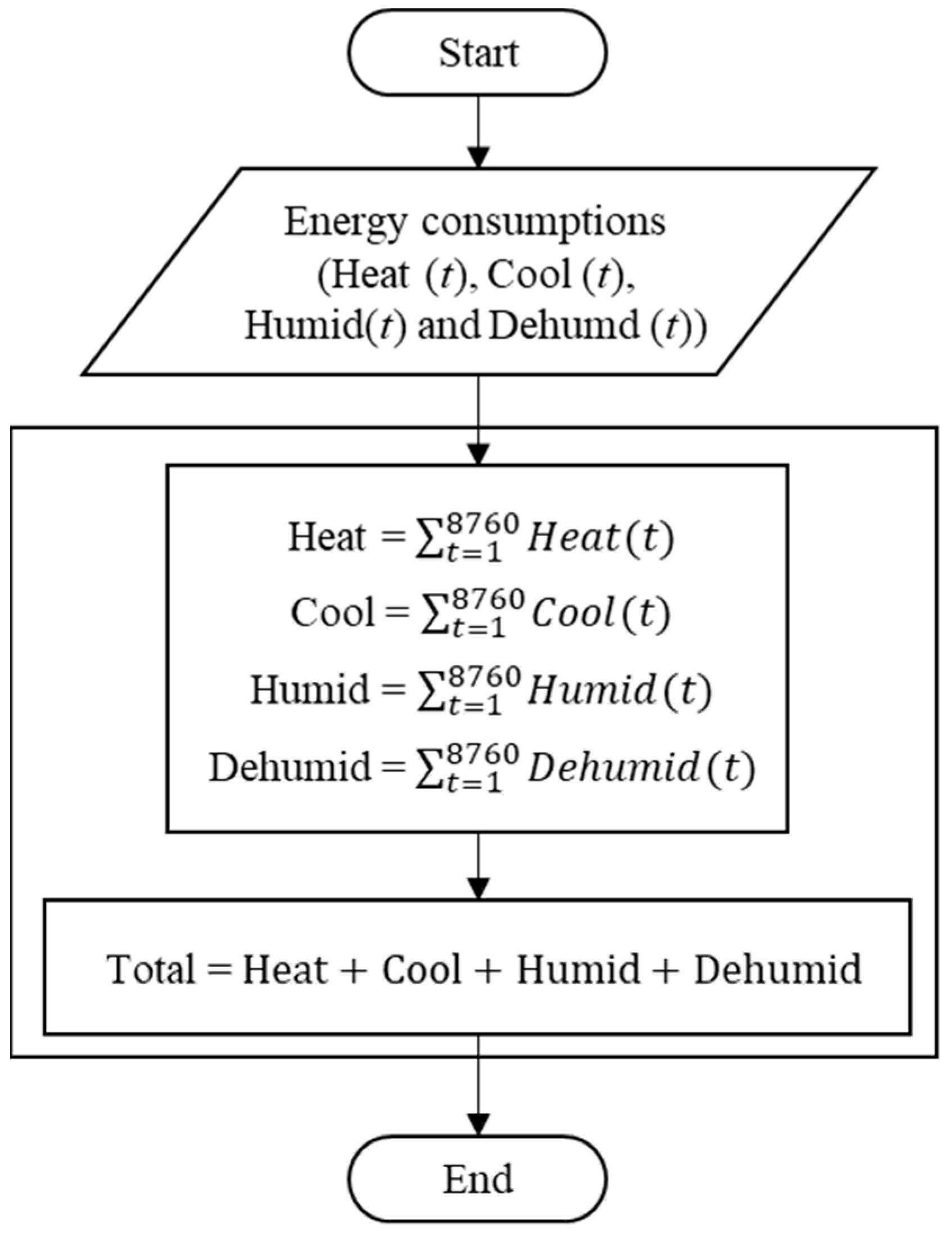
Figure A2.
Procedure for quantifying the energy consumptions developed in MATLAB.
Figure A2.
Procedure for quantifying the energy consumptions developed in MATLAB.
References
- Nakicenovic, N.; Alcamo, J.; Davis, G.; de Vries, B.; Fenhann, J.; Gaffin, S.; Gregory, K.; Griibler, A.; Jung, T.Y.; Kram, T.; et al. Special Report on Emissions Scenarios—A Special Report of Working Group III of the Intergovernmental Panel on Climate Change; Cambridge University Press: Cambridge, UK, 2000. [Google Scholar]
- de Wilde, P.; Coley, D. The implications of a changing climate for buildings. Build. Environ. 2012, 55, 1–7. [Google Scholar] [CrossRef]
- OECD Stat Greenhouse Gas Emissions. Available online: https://stats.oecd.org/Index.aspx?DataSetCode=AIR_GHG# (accessed on 30 January 2023).
- European Commission. Climate Strategies & Targets. Available online: https://ec.europa.eu/clima/policies/strategies/2020_en (accessed on 30 January 2023).
- Eurostat. Emissions of Greenhouse Gases and Air Pollutants from Final Use of CPA08 Products—Input-Output Analysis. Available online: https://appsso.eurostat.ec.europa.eu/nui/show.do?dataset=env_ac_io10&lang=en (accessed on 16 September 2019).
- Paris Agreement. Available online: https://unfccc.int/process-and-meetings/the-paris-agreement/the-paris-agreement (accessed on 30 January 2023).
- EnergyPlus. EnergyPlus, version 8.8.0; U.S. Department of Energy’s (DOE)—Building Technologies Office (BTO): Washington, DC, USA, 2017.
- Fraunhofer Institute for Building Physics. WUFI®Plus, version 3.1.1.0; Fraunhofer Institute for Building Physics: Stuttgart, Germany, 2017. [Google Scholar]
- Andarini, R. The Role of Building Thermal Simulation for Energy Efficient Building Design. Energy Procedia 2014, 47, 217–226. [Google Scholar] [CrossRef]
- Giuseppe, E.D.; D’Orazio, M.; Favi, C.; Rossi, M.; Lasvaux, S.; Padey, P.; Favre, D.; Wittchen, K.; Du, G.; Nielsen, A.; et al. Report and Tool: Probability Based Life Cycle Impact Assessment, Robust Internal Thermal Insulation of Historic Buildings (RIBuild Project)—Project No. 637268; RIBuild: Copenhagen, Denmark, 2019. [Google Scholar]
- Antretter, F.; Schöpfer, T.; Kilian, R. An approach to assess future climate change effects on indoor climate of a historic stone church. In Proceedings of the 9th Nordic Symposium on Building Physics, Tampere, Finland, 29 May–2 June 2011. [Google Scholar]
- Coelho, G.B.A.; Silva, H.E.; Henriques, F.M.A. Impact of climate change on cultural heritage: A simulation study to assess the risks for conservation and thermal comfort. Int. J. Glob. Warm. 2019, 19, 382. [Google Scholar] [CrossRef]
- Huijbregts, Z.; Kramer, R.P.; Martens, M.H.J.; van Schijndel, A.W.M.; Schellen, H.L. A proposed method to assess the damage risk of future climate change to museum objects in historic buildings. Build. Environ. 2012, 55, 43–56. [Google Scholar] [CrossRef]
- Rajčić, V.; Skender, A.; Damjanović, D. An innovative methodology of assessing the climate change impact on cultural heritage. Int. J. Archit. Herit. 2017, 12, 1–15. [Google Scholar] [CrossRef]
- Choidis, P.; Kraniotis, D.; Lehtonen, I.; Hellum, B. A Modelling Approach for the Assessment of Climate Change Impact on the Fungal Colonization of Historic Timber Structures. Forests 2021, 12, 819. [Google Scholar] [CrossRef]
- Coelho, G.B.A.; Silva, H.E.; Henriques, F.M.A. Calibrated hygrothermal simulation models for historical buildings. Build. Environ. 2018, 142, 439–450. [Google Scholar] [CrossRef]
- Silva, H.E.; Henriques, F.M.A. Microclimatic analysis of historic buildings: A new methodology for temperate climates. Build. Environ. 2014, 82, 381–387. [Google Scholar] [CrossRef]
- Barbosa, F.C.; de Freitas, V.P.; Almeida, M. School building experimental characterization in Mediterranean climate regarding comfort, indoor air quality and energy consumption. Energy Build. 2020, 212, 109782. [Google Scholar] [CrossRef]
- Barbosa, F.C.; de Freitas, V.P.; Almeida, M. Strategies for school buildings refurbishment in Portuguese climate. E3S Web Conf. 2020, 172, 18007. [Google Scholar] [CrossRef]
- Wang, F.; Pichetwattana, K.; Hendry, R.; Galbraith, R. Thermal performance of a gallery and refurbishment solutions. Energy Build. 2014, 71, 38–52. [Google Scholar] [CrossRef]
- Leissner, J.; Kilian, R.; Kotova, L.; Jacob, D.; Mikolajewicz, U.; Broström, T.; Smith, J.A.; Schellen, H.L.; Martens, M.; Schijndel, J.V.; et al. Climate for Culture: Assessing the impact of climate change on the future indoor climate in historic buildings using simulations. Herit. Sci. 2015, 3, 1–15. [Google Scholar] [CrossRef]
- Kramer, R.P.; Maas, M.P.E.; Martens, M.H.J.; van Schijndel, A.W.M.; Schellen, H.L. Energy conservation in museums using different setpoint strategies: A case study for a state-of-the-art museum using building simulations. Appl. Energy 2015, 158, 446–458. [Google Scholar] [CrossRef]
- Climate Change—SPM Synthesis Report—Summary for Policymakers (SPM). Contribution of Working Groups I, II and III to the Fifth Assessment Report of the Intergovernmental Panel on Climate Change; Core Writing Team, Pachauri, R.K., Meyer, L.A., Eds.; IPCC: Geneva, Switzerland, 2014. [Google Scholar] [CrossRef]
- Roberti, F.; Oberegger, U.F.; Gasparella, A. Calibrating historic building energy models to hourly indoor air and surface temperatures: Methodology and case study. Energy Build. 2015, 108, 236–243. [Google Scholar] [CrossRef]
- Schmidt, E.D.; Sciurpi, F.; Carletti, C.; Cellai, G.; Pierangioli, L.; Russo, G. The BEM of the Vasari Corridor: A return to its original function and correlated energy consumption for artwork conservation and IAQ. Sci. Technol. Built Environ. 2021, 27, 1104–1126. [Google Scholar] [CrossRef]
- Giuliani, M.; Henze, G.P.; Florita, A.R. Modelling and calibration of a high-mass historic building for reducing the prebound effect in energy assessment. Energy Build. 2016, 116, 434–448. [Google Scholar] [CrossRef]
- WUFI-Wiki Physical Background for WUFI® PRO, 2D & Plus. Available online: https://www.wufi-wiki.com/mediawiki/index.php/Details:Physics (accessed on 13 September 2020).
- Coelho, G.B.A.; Silva, H.E.; Henriques, F.M.A. Impact of climate change in cultural heritage: From energy consumption to artefacts’ conservation and building rehabilitation. Energy Build. 2020, 224, 110250. [Google Scholar] [CrossRef]
- Martens, M. Climate Risk Assessment in Museums: Degradation Risks Determined from Temperature and Relative Humidity Data. Ph.D. Thesis, Technische Universiteit Eindhoven, Eindhoven, The Netherlands, 2012. [Google Scholar]
- Muñoz-González, C.M.; León-Rodríguez, A.L.; Navarro-Casas, J. Air conditioning and passive environmental techniques in historic churches in Mediterranean climate. A proposed method to assess damage risk and thermal comfort pre-intervention, simulation-based. Energy Build. 2016, 130, 567–577. [Google Scholar] [CrossRef]
- Kramer, R.P.; van Schijndel, J.; Schellen, H. Dynamic setpoint control for museum indoor climate conditioning integrating collection and comfort requirements: Development and energy impact for Europe. Build. Environ. 2017, 118, 14–31. [Google Scholar] [CrossRef]
- Posani, M.; Veiga, R.; de Freitas, V.P. Retrofitting historic walls: Feasibility of thermal insulation and suitability of thermal mortars. Heritage 2021, 4, 114. [Google Scholar] [CrossRef]
- Posani, M.; Veiga, R.; de Freitas, V.P. Thermal mortar-based insulation solutions for historic walls: An extensive hygrothermal characterization of materials and systems. Constr. Build. Mater. 2022, 315, 125640. [Google Scholar] [CrossRef]
- Coelho, G.B.A. Optimization of Historic Buildings that House Artefacts Considering Climate Change. Ph.D. Thesis, FCT-UNL, Lisbon, Portugal, 2020. [Google Scholar]
- Silva, H.; Henriques, F.M.A. Preventive conservation of historic buildings in temperate climates. The importance of a risk-based analysis on the decision-making process. Energy Build. 2015, 107, 26–36. [Google Scholar] [CrossRef]
- Monsalve, M. Igreja Paroquial de S. Cristóvão—Relatório de Inventário e Diagnóstico. 2011. Available online: http://portal.iphan.gov.br/uploads/ckfinder/arquivos/Relat%C3%B3rio%20de%20Gest%C3%A3o%20%202011.pdf (accessed on 13 January 2023).
- Coelho, G.B.A.; Silva, H.E.; Henriques, F.M.A. Development of a hygrothermal model of a historic building in WUFI®Plus vs. EnergyPlus. In Proceedings of the 4th Central European Symposium on Building Physics (CESBP 2019), Prague, Czech Republic, 2–5 September 2019. [Google Scholar]
- American Society of Heating Refrigerating and Air-Conditioning Engineers (ASHRAE). ASHRAE Guideline 14:2002, Measurement of Energy and Demand Savings, Proceedings of the Fifth International Conference for Enhanced Building Operations, Pittsburgh, PA, USA, 11–13 October 2005; Energy Systems Laboratory, Texas A&M University: College Station, TX, USA, 2005. [Google Scholar]
- Coelho, G.B.A.; Henriques, F.M.A. Performance of passive retrofit measures for historic buildings that house artefacts viable for future conditions. Sustain. Cities Soc. 2021, 71, 102982. [Google Scholar] [CrossRef]
- Nishimura, D.W. Understanding Preservation Metrics; Image Permanence Institute (IPI): New York, NY, USA, 2007; Volume 11. [Google Scholar]
- Sedlbauer, K. Prediction of Mould Fungus Formation on the Surface of and Inside Building Components. Ph.D. Thesis, Fraunhofer Institute for Building Physics, Stuttgart, Germany, 2001. [Google Scholar]
- Michalski, S. Double the life for each five-degree drop, more than double the life for each halving of relative humidity. In Proceedings of the Thirteenth Triennial Meeting ICOM-CC, Rio de Janeiro, Brazil, 22–27 September 2002; Volume I, pp. 66–72. [Google Scholar]
- Bratasz, L.; Kozlowski, R.; Kozlowska, A.; Rivers, S. Conservation of the Mazarin Chest: Structural response of Japanese lacquer to variations in relative humidity. In Proceedings of the 15th Triennial Conference, New Delhi, India, 22–26 September 2008; pp. 1086–1093. [Google Scholar]
- Jakieła, S.; Bratasz, R. Kozłowski, Numerical modelling of moisture movement and related stress field in lime wood subjected to changing climate conditions. Wood Sci. Technol. 2008, 42, 21–37. [Google Scholar] [CrossRef]
- Mecklenburg, M.F.; Tumosa, C.S.; Erhardt, D. Structural response of painted wood surfaces to changes in ambient relative humidity. In Structural Response of Painted Wood Surfaces to Changes in Ambient RH; The Getty Conservation Institute: Los Angeles, CA, USA, 1998; pp. 464–483. [Google Scholar]
- Bratasz, Ł.; Kozłowski, R.; Lasyk, Ł. Allowable microclimatic variations for painted wood: Numerical modelling and direct tracing of the fatigue damage. In Proceedings of the ICOM CC 16th Triennial Conference, Lizbona, Portugal, 19–23 September 2011. [Google Scholar]
- WMO. Calculation of Monthly and Annual 30-Year Standard Normals, Proceedings of the Meeting of experts, Washington, DC, USA, March 1989; WCDP 10 and WMOTD 341; World Meteorological Organization: Geneva, Switzerland, 1989; p. 14. [Google Scholar]
- CORDEX-2. Coordinated Regional Climate Downscalling Experiment (CORDEX). Available online: http://www.cordex.org/ (accessed on 17 January 2019).
- EN ISO 15927-4; Hygrothermal Performance of Buildings—Calculation and Presentation of Climatic Data—Part 4: Hourly Data for Assessing the Annual Energy Use for Heating and Cooling. European Commitee for Standardization (CEN): Brussels, UK, 2005; p. 16.
- Skartveit, A.; Olseth, J.A.; Tuft, M.E. An hourly diffuse fraction model with correction for variability and surface albedo. Sol. Energy 1998, 63, 173–183. [Google Scholar] [CrossRef]
- Lanini, F. Division of Global Radiation into Direct Radiation and Diffuse Radiation. Master’s Dissertation, Faculty of Science, University of Bern, Bern, Switzerland, 2010. [Google Scholar]
- MediaWorkstations a-X—AMD Threadripper Workstation for CPU and GPU Rendering. Available online: https://www.mediaworkstations.net/systems/amd-workstations/a-x/ (accessed on 10 September 2020).
- Silva, H.E. Indoor Climate Management on Cultural Heritage Buildings: Climate Control Strategies, Cultural Heritage Management and Hygrothermal Rehabilitation. Ph.D. Thesis, Faculdade de Ciências e Tecnologia, Universidade NOVA de Lisboa (FCT-UNL), Lisbon, Portugal, 2019. [Google Scholar]
- Almeida, R.M.S.F.; Freitas, V.P. An insulation thickness optimization methodology for school buildings rehabilitation combining artificial neural networks and life cycle cost. J. Civ. Eng. Manag. 2016, 22, 915–923. [Google Scholar] [CrossRef]
- Asadi, E.; Silva, M.G.D.; Antunes, C.H.; Dias, L.; Glicksman, L. Multi-objective optimization for building retrofit: A model using genetic algorithm and artificial neural network and an application. Energy Build. 2014, 81, 444–456. [Google Scholar] [CrossRef]
- Silva, H.E.; Henriques, F.M.A.; Henriques, T.A.S.; Coelho, G. A sequential process to assess and optimize the indoor climate in museums. Build. Environ. 2016, 104, 21–34. [Google Scholar] [CrossRef]

Disclaimer/Publisher’s Note: The statements, opinions and data contained in all publications are solely those of the individual author(s) and contributor(s) and not of MDPI and/or the editor(s). MDPI and/or the editor(s) disclaim responsibility for any injury to people or property resulting from any ideas, methods, instructions or products referred to in the content. |
© 2023 by the authors. Licensee MDPI, Basel, Switzerland. This article is an open access article distributed under the terms and conditions of the Creative Commons Attribution (CC BY) license (https://creativecommons.org/licenses/by/4.0/).