
Assessment of the Rock Elasticity Modulus Using Four Hybrid RF Models: A Combination of Data-Driven and Soft Techniques


Abstract
:1. Introduction
2. Data Preparation
3. Development of Hybrid RF Models for Predicting the Rock EM
3.1. Metaheuristic Optimization Algorithms
3.1.1. Backtracking Search Optimization Algorithm (BSA)
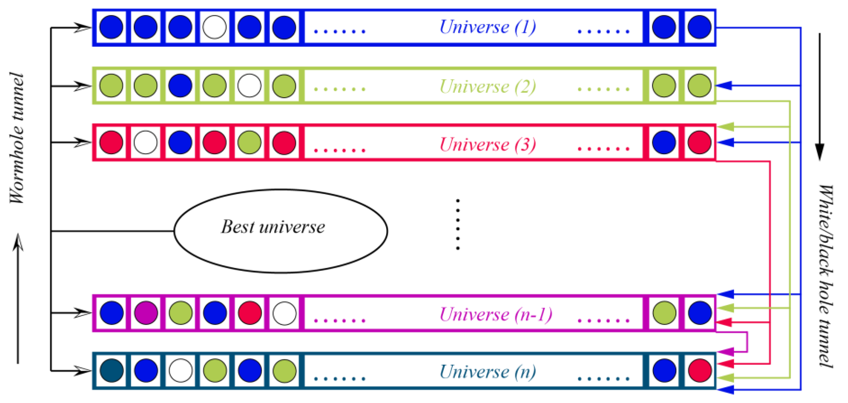
3.1.2. Multi-Verse Optimizer (MVO)
- (1)
- Population—the initial population of the universes in the searching space is defined using the Equation (6).
- (2)
- Exploration and exploitation—the function of wormholes is to help objects move from one universe to another (see Figure 2). Thus, this mechanism by which objects are exchanged between universes through wormholes can be described as:
3.1.3. Golden Eagle Optimizer (GEO)
- (I)
- Selecting the prey—the selection can occur in a basic way, with each golden eagle randomly select a prey from the memory of any other group member to better explore the landscape. It is important to note that the chosen prey is not necessarily the nearest or furthest prey. Figure 3 shows how prey selection works.
- (II)
- Exploration and exploitation—after determining the prey, each golden eagle carries out the attacking and cruising behaviors. The attacking behavior can be expressed by the following mathematical formula:
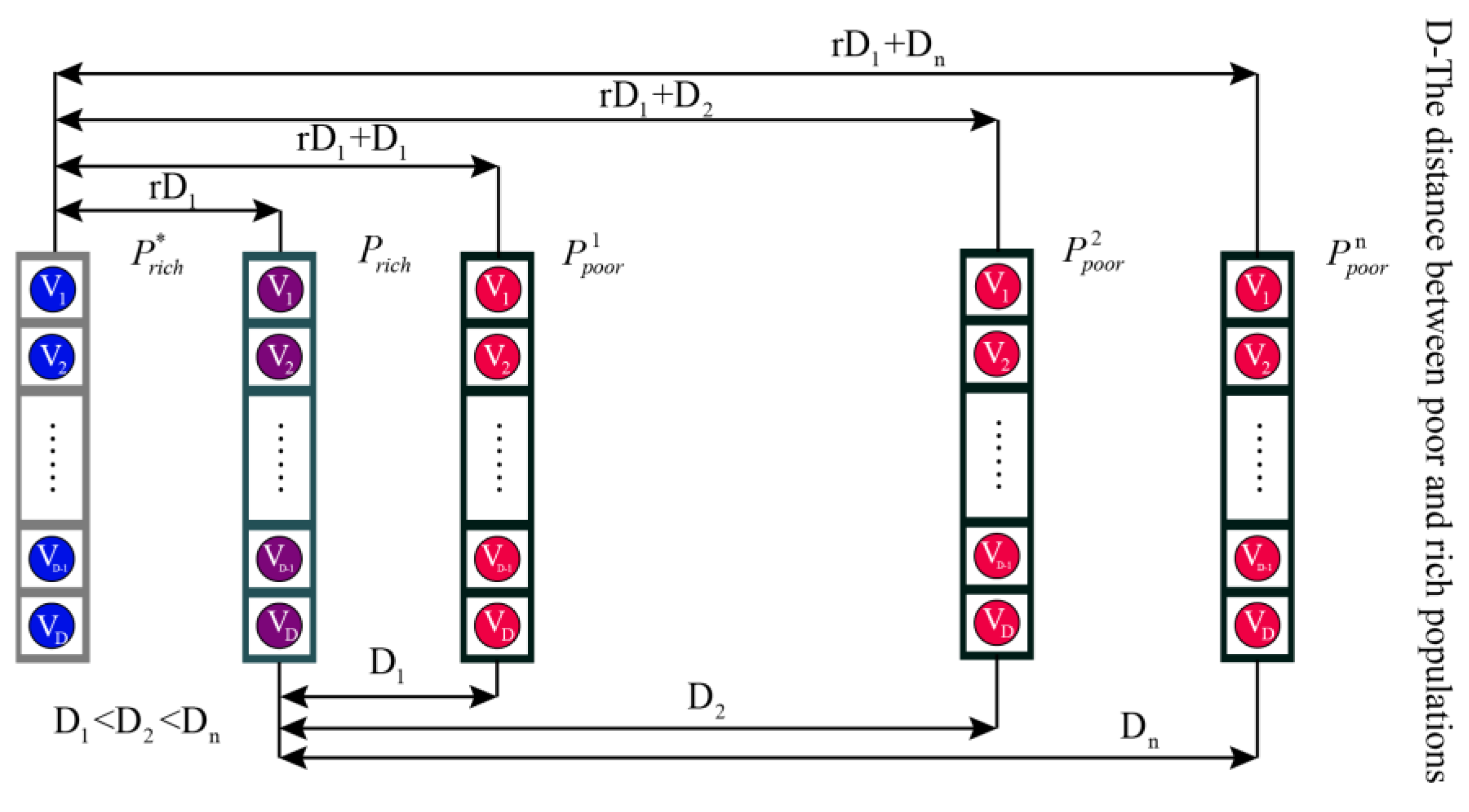
3.1.4. Poor and Rich Optimization Algorithm (PRO)
3.2. Hybrid RF Models
- (i)
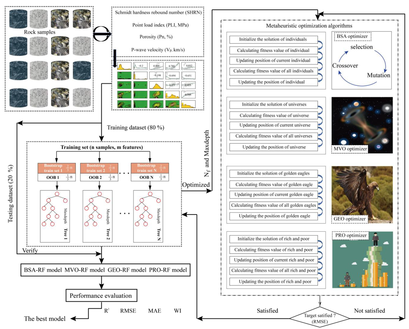
- Data preprocessingA total of 120 rock samples with four input variables were used to predict the EM in this paper. All variables need to be extracted and normalized to [−1, 1]. The purpose of this step is to prevent a failure for establishing the accurate prediction relationships due to the parameter variability. After that, the train and test sets are separated from the initial database. The ratio of the train set to the test set is set equal to 4 to 1. It should be noted that the same train or test set is used to generate each hybrid RF model for predicting the rock EM and comparing their performance.
- (ii)
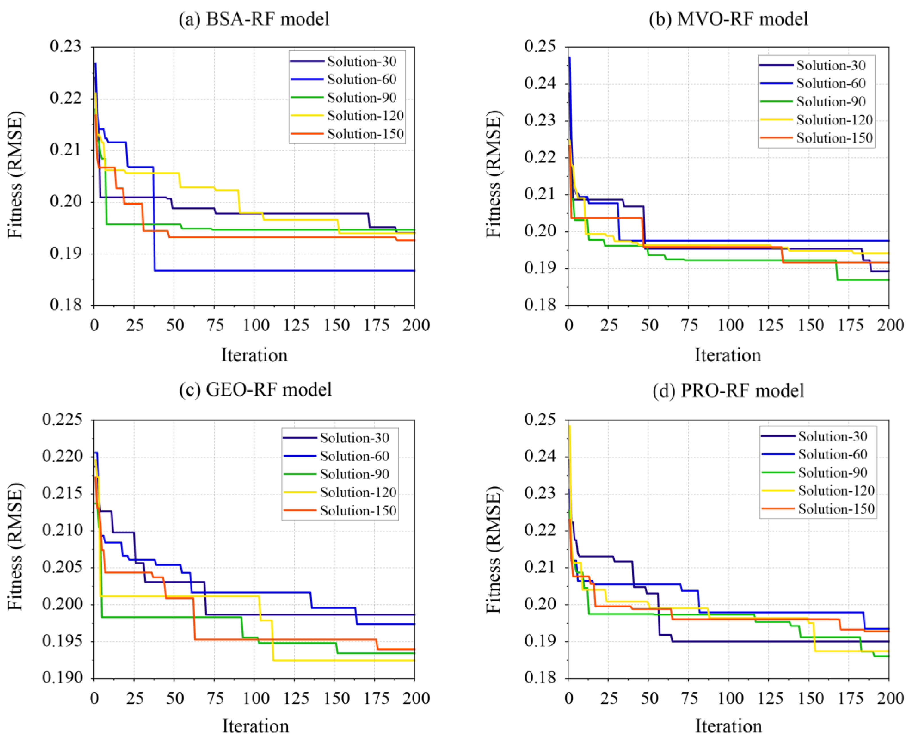
- Parameter settingsAlthough the Nt increase will not cause an overfitting of the RF model, a large parameter selection range can greatly increase the computation time. Therefore, the ranges of Nt and Maxdepth are set equal to [1, 100] and [1, 10], respectively. For the four MOA algorithms, the number of initial solutions (i.e., individuals of BSA, candidates of MVO, population of GEO and human of PRO) and the iteration time are the core factors that affect the optimization performance of these algorithms. To better activate the optimization performance, the solutions are set equal to 30, 60, 90, 120 and 150 during the 200 iterations.
- (iii)
- Optimization evaluationThe fitness function is utilized to evaluate the performance of each hybrid RF model with different solutions during the 200 iterations. The RMSE is adopted to represent the fitness values of all models in this paper. They do not need an absolute value to evaluate the model performance [51]. In other words, the best-optimized RF model has the lowest RMSE value among all hybrid models based on the same MOA. The flowchart for developing four hybrid RF models for predicting the rock EM is shown in Figure 5.
4. Performance Evaluation
5. Results and Discussion
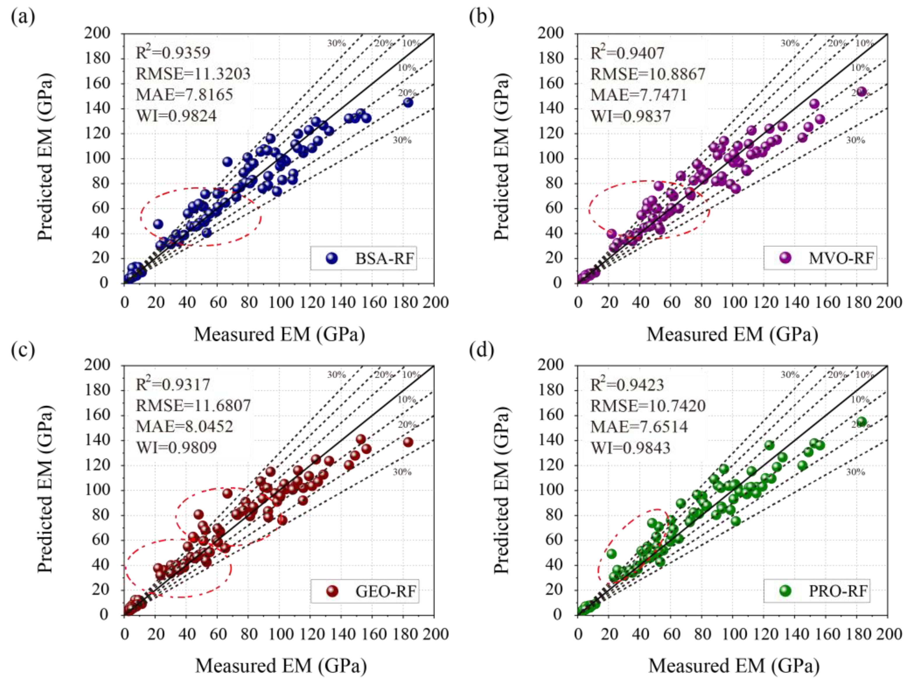
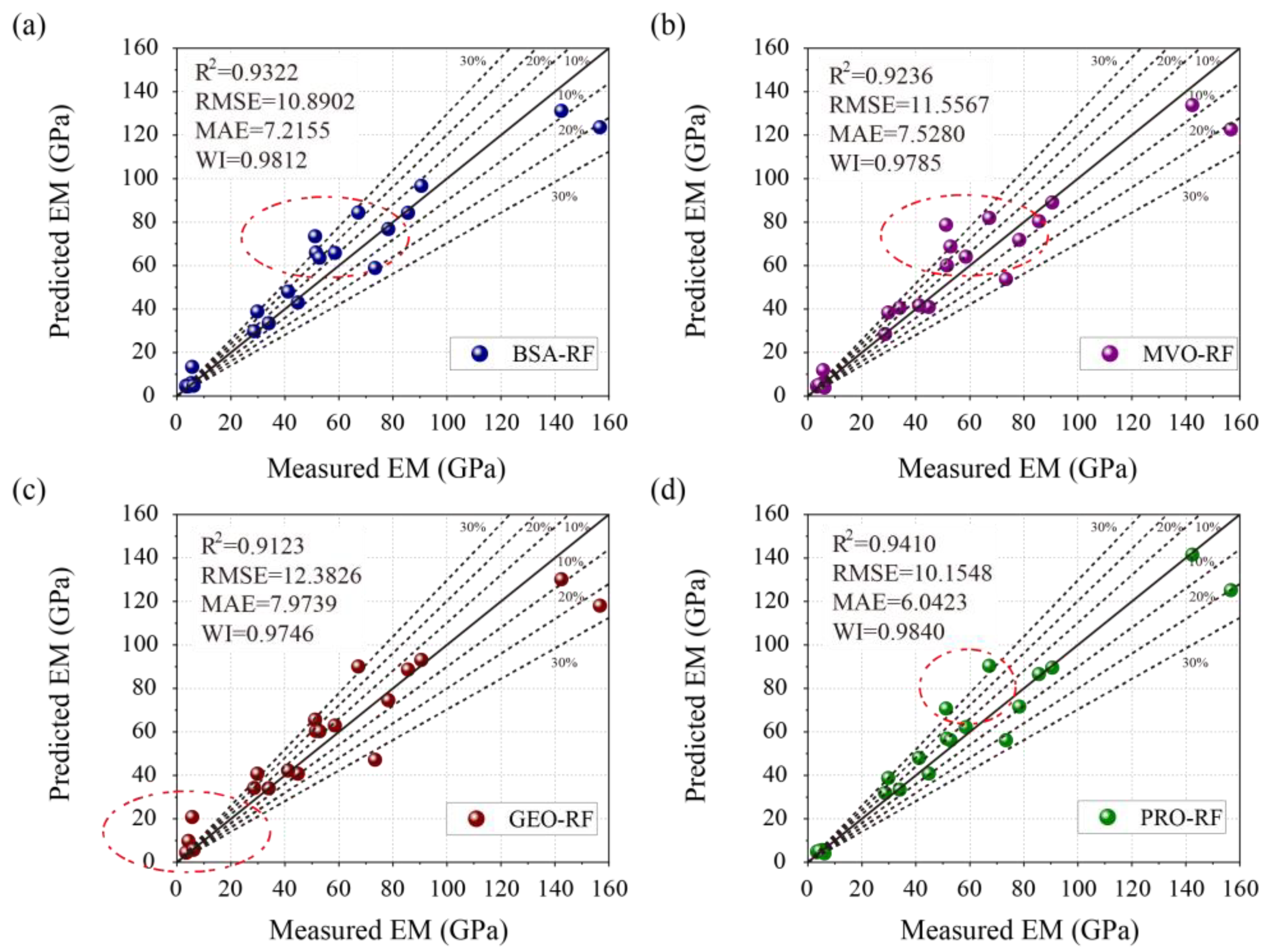
5.1. Results of the Proposed Four Hybrid Models
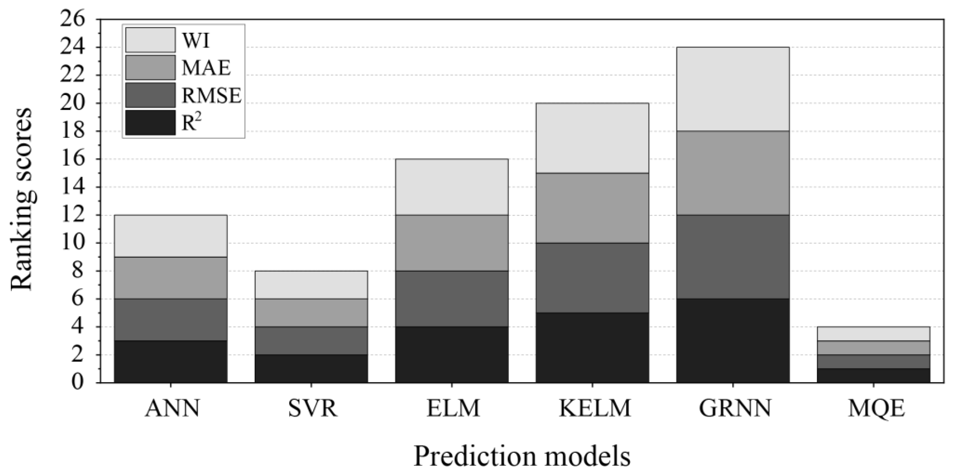
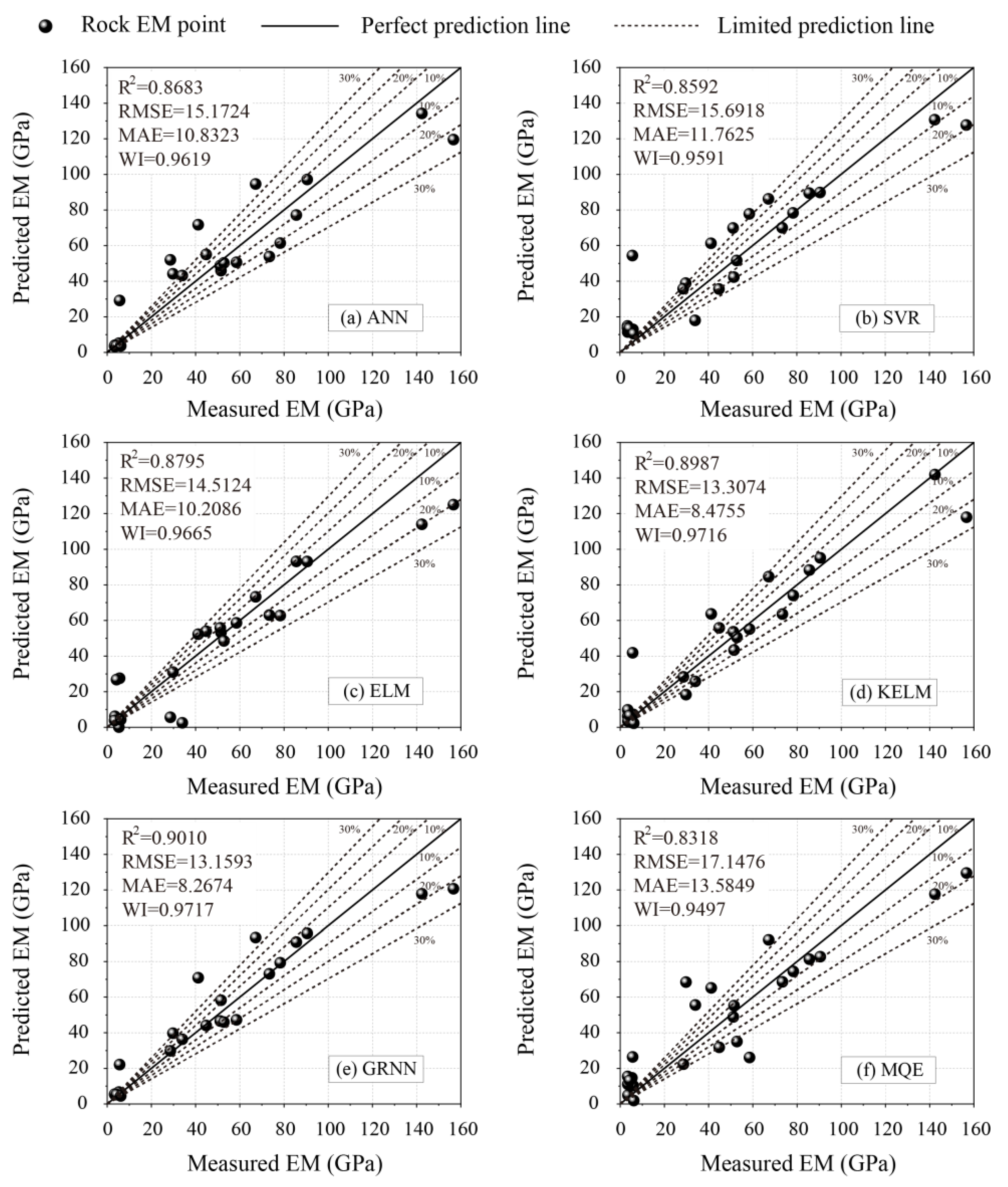
5.2. Performance Comparison between the Proposed and Other Models
5.3. Sensitive Analysis
6. Conclusions
- i.
- Four hybrid RF models have obtained a good prediction accuracy by means of four performance indices. In particular, the PRO-RF model is the best model among them.
- ii.
- The GRNN model has a better predictive performance than the other ML models and the empirical formula. It results in the higher values of R2 (0.9010) and WI (0.9717) and the lower values of RMSE (13.1593) and MAE (8.2674). However, these four optimized RF models are superior to the GRNN model.
- iii.
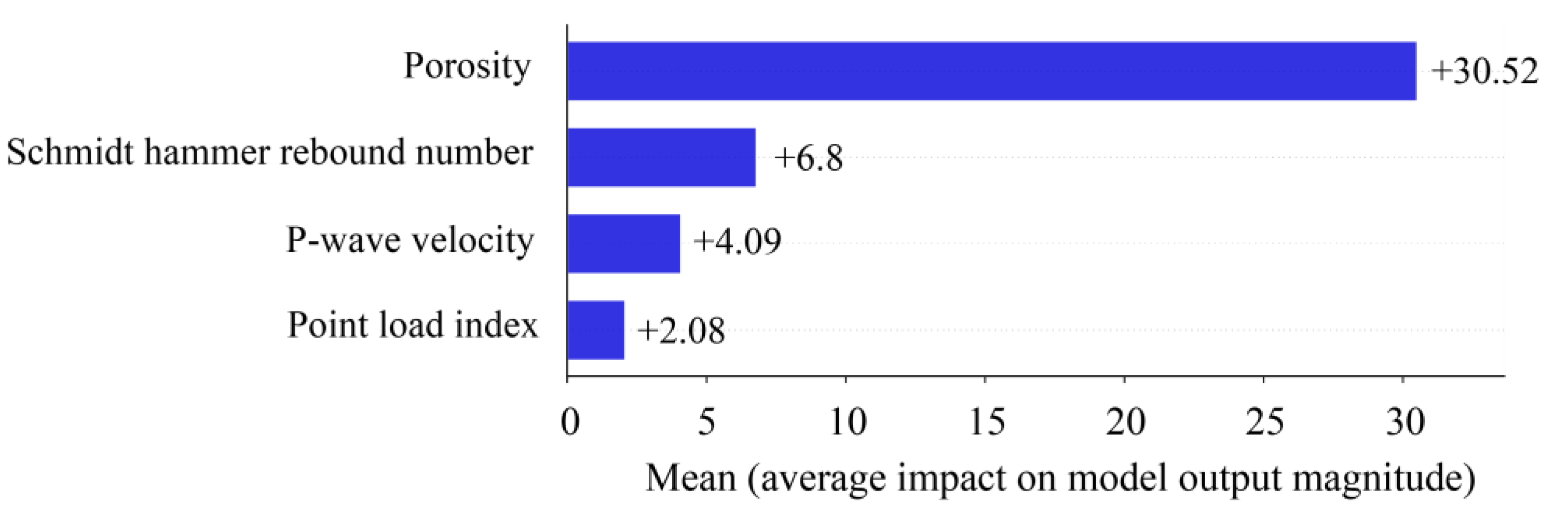
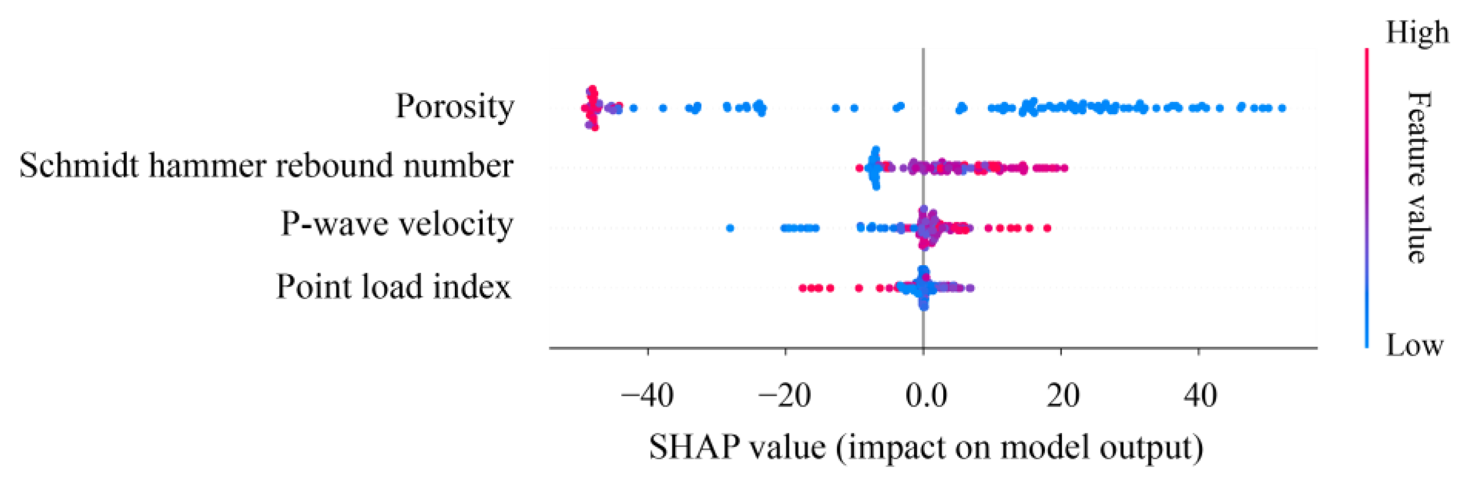
- The porosity (Pn) is the most important variable by means of the highest average impact value of 30.52 for predicting the rock EM. Meanwhile, the Pn is also the only variable negatively correlated with EM.
Author Contributions
Funding
Institutional Review Board Statement
Informed Consent Statement
Data Availability Statement
Conflicts of Interest
References
- Ersoy, H.; Kanik, D. Multicriteria decision-making analysis based methodology for predicting carbonate rocks’ uniaxial compressive strength. Earth Sci. Res. J. 2012, 16, 65–74. [Google Scholar]
- Armaghani, D.J.; Tonnizam Mohamad, E.; Momeni, E.; Narayanasamy, M.S. An adaptive neuro-fuzzy inference system for predicting unconfined compressive strength and Young’s modulus: A study on Main Range granite. Bull. Eng. Geol. Environ. 2015, 74, 1301–1319. [Google Scholar] [CrossRef]
- Armaghani, D.J.; Tonnizam Mohamad, E.; Momeni, E.; Monjezi, M.; Sundaram Narayanasamy, M. Prediction of the strength and elasticity modulus of granite through an expert artificial neural network. Arab. J. Geosci. 2016, 9, 48. [Google Scholar] [CrossRef]
- Madhubabu, N.; Singh, P.K.; Kainthola, A.; Mahanta, B.; Tripathy, A.; Singh, T.N. Prediction of compressive strength and elastic modulus of carbonate rocks. Measurement 2016, 88, 202–213. [Google Scholar] [CrossRef]
- Nasiri, H.; Homafar, A.; Chelgani, S.C. Prediction of uniaxial compressive strength and modulus of elasticity for Travertine samples using an explainable artificial intelligence. Results Geophys. Sci. 2021, 8, 100034. [Google Scholar] [CrossRef]
- Jamshidi, A.; Nikudel, M.R.; Khamehchiyan, M.; Sahamieh, R.Z. The effect of specimen diameter size on uniaxial compressive strength, P-wave velocity and the correlation between them. Geomech. Geoengin. 2016, 11, 13–19. [Google Scholar] [CrossRef]
- Sonmez, H.; Gokceoglu, C.; Nefeslioglu, H.A.; Kayabasi, A. Estimation of rock modulus: For intact rocks with an artificial neural network and for rock masses with a new empirical equation. Int. J. Rock Mech. Min. Sci. 2006, 43, 224–235. [Google Scholar] [CrossRef]
- Palchik, V. On the ratios between elastic modulus and uniaxial compressive strength of heterogeneous carbonate rocks. Rock Mech. Rock Eng. 2011, 44, 121–128. [Google Scholar] [CrossRef]
- Najibi, A.R.; Ghafoori, M.; Lashkaripour, G.R.; Asef, M.R. Empirical relations between strength and static and dynamic elastic properties of Asmari and Sarvak limestones, two main oil reservoirs in Iran. J. Pet. Sci. Eng. 2015, 126, 78–82. [Google Scholar] [CrossRef]
- Hoek, E.; Diederichs, M.S. Empirical estimation of rock mass modulus. Int. J. Rock Mech. Min. Sci. 2006, 43, 203–215. [Google Scholar] [CrossRef]
- Alemdag, S.; Gurocak, Z.; Gokceoglu, C. A simple regression based approach to estimate deformation modulus of rock masses. J. Afr. Earth Sci. 2015, 110, 75–80. [Google Scholar] [CrossRef]
- Kayabasi, A.; Gokceoglu, C. Deformation modulus of rock masses: An assessment of the existing empirical equations. Geotech. Geol. Eng. 2018, 36, 2683–2699. [Google Scholar] [CrossRef]
- Yilmaz, I.; Yuksek, G. Prediction of the strength and elasticity modulus of gypsum using multiple regression, ANN, and ANFIS models. Int. J. Rock Mech. Min. Sci. 2009, 46, 803–810. [Google Scholar] [CrossRef]
- Moradian, Z.A.; Behnia, M. Predicting the uniaxial compressive strength and static Young’s modulus of intact sedimentary rocks using the ultrasonic test. Int. J. Geomech. 2009, 9, 14. [Google Scholar] [CrossRef]
- Yılmaz, I.; Sendır, H. Correlation of Schmidt hardness with unconfined compressive strength and Young’s modulus in gypsum from Sivas (Turkey). Eng. Geol. 2002, 66, 211–219. [Google Scholar] [CrossRef]
- Saedi, B.; Mohammadi, S.D.; Shahbazi, H. Application of fuzzy inference system to predict uniaxial compressive strength and elastic modulus of migmatites. Environ. Earth Sci. 2019, 78, 208. [Google Scholar] [CrossRef]
- Beiki, M.; Majdi, A.; Givshad, A.D. Application of genetic programming to predict the uniaxial compressive strength and elastic modulus of carbonate rocks. Int. J. Rock Mech. Min. Sci. 2013, 63, 159–169. [Google Scholar] [CrossRef]
- Yasar, E.; Erdogan, Y. Correlating sound velocity with the density, compressive strength and Young’s modulus of carbonate rocks. Int. J. Rock Mech. Min. Sci. 2004, 41, 871–875. [Google Scholar] [CrossRef]
- Dinçer, I.; Acar, A.; Çobanoğlu, I.; Uras, Y. Correlation between Schmidt hardness, uniaxial compressive strength and Young’s modulus for andesites, basalts and tuffs. Bull. Eng. Geol. Environ. 2004, 63, 141–148. [Google Scholar] [CrossRef]
- Behzadafshar, K.; Sarafraz, M.E.; Hasanipanah, M.; Mojtahedi, S.F.F.; Tahir, M.M. Proposing a new model to approximate the elasticity modulus of granite rock samples based on laboratory tests results. Bull. Eng. Geol. Environ. 2019, 78, 1527–1536. [Google Scholar] [CrossRef]
- Dehghan, S.; Sattari, G.H.; Chelgani, S.C.; Aliabadi, M.A. Prediction of uniaxial compressive strength and modulus of elasticity for Travertine samples using regression and artificial neural networks. Min. Sci. Technol. 2010, 20, 41–46. [Google Scholar] [CrossRef]
- Rezaei, M.; Majdi, A.; Monjezi, M. An intelligent approach to predict unconfined compressive strength of rock surrounding access tunnels in longwall coal mining. Neural Comput. Appl. 2014, 24, 233–241. [Google Scholar] [CrossRef]
- Jin, X.; Zhao, R.; Ma, Y. Application of a Hybrid Machine Learning Model for the Prediction of Compressive Strength and Elastic Modulus of Rocks. Minerals 2022, 12, 1506. [Google Scholar] [CrossRef]
- Ceryan, N.; Ozkat, E.C.; Korkmaz Can, N.; Ceryan, S. Machine learning models to estimate the elastic modulus of weathered magmatic rocks. Environ. Earth Sci. 2021, 80, 448. [Google Scholar] [CrossRef]
- Shahani, N.M.; Zheng, X.; Liu, C.; Hassan, F.U.; Li, P. Developing an XGBoost regression model for predicting young’s modulus of intact sedimentary rocks for the stability of surface and subsurface structures. Front. Earth Sci. 2021, 9, 761990. [Google Scholar] [CrossRef]
- Li, C.; Zhou, J.; Dias, D.; Gui, Y. A Kernel Extreme Learning Machine-Grey Wolf Optimizer (KELM-GWO) Model to Predict Uniaxial Compressive Strength of Rock. Appl. Sci. 2022, 12, 8468. [Google Scholar] [CrossRef]
- Elkatatny, S.; Tariq, Z.; Mahmoud, M.; Abdulraheem, A.; Mohamed, I. An integrated approach for estimating static Young’s modulus using artificial intelligence tools. Neural Comput. Appl. 2019, 31, 4123–4135. [Google Scholar] [CrossRef]
- Aboutaleb, S.; Behnia, M.; Bagherpour, R.; Bluekian, B. Using non-destructive tests for estimating uniaxial compressive strength and static Young’s modulus of carbonate rocks via some modeling techniques. Bull. Eng. Geol. Environ. 2018, 77, 1717–1728. [Google Scholar] [CrossRef]
- Siddig, O.; Elkatatny, S. Workflow to build a continuous static elastic moduli profile from the drilling data using artificial intelligence techniques. J. Pet. Explor. Prod. Technol. 2021, 11, 3713–3722. [Google Scholar] [CrossRef]
- Mei, X.; Li, C.; Sheng, Q.; Cui, Z.; Zhou, J.; Dias, D. Development of a hybrid artificial intelligence model to predict the uniaxial compressive strength of a new aseismic layer made of rubber-sand concrete. Mech. Adv. Mater. Struct. 2022, 1–18. [Google Scholar] [CrossRef]
- Ocak, I.; Seker, S.E. Estimation of elastic modulus of intact rocks by artificial neural network. Rock Mech. Rock Eng. 2012, 45, 1047–1054. [Google Scholar] [CrossRef]
- Pappalardo, G.; Mineo, S. Static elastic modulus of rocks predicted through regression models and Artificial Neural Network. Eng. Geol. 2022, 308, 106829. [Google Scholar] [CrossRef]
- Singh, R.; Kainthola, A.; Singh, T.N. Estimation of elastic constant of rocks using an ANFIS approach. Appl. Soft Comput. 2012, 12, 40–45. [Google Scholar] [CrossRef]
- Umrao, R.K.; Sharma, L.K.; Singh, R.; Singh, T.N. Determination of strength and modulus of elasticity of heterogenous sedimentary rocks: An ANFIS predictive technique. Measurement 2018, 126, 194–201. [Google Scholar] [CrossRef]
- Acar, M.C.; Kaya, B. Models to estimate the elastic modulus of weak rocks based on least square support vector machine. Arab. J. Geosci. 2020, 13, 590. [Google Scholar] [CrossRef]
- Al-Anazi, A.F.; Gates, I.D. On support vector regression to predict Poisson’s ratio and Young’s Modulus of reservoir rock. In Artificial Intelligent Approaches in Petroleum Geosciences; Springer: Cham, Switzerland, 2015; pp. 167–189. [Google Scholar]
- Matin, S.S.; Farahzadi, L.; Makaremi, S.; Chelgani, S.C.; Sattari, G.H. Variable selection and prediction of uniaxial compressive strength and modulus of elasticity by random forest. Appl. Soft Comput. 2018, 70, 980–987. [Google Scholar] [CrossRef]
- Khan, N.M.; Cao, K.; Yuan, Q.; Bin Mohd Hashim, M.H.; Rehman, H.; Hussain, S.; Khan, S. Application of Machine Learning and Multivariate Statistics to Predict Uniaxial Compressive Strength and Static Young’s Modulus Using Physical Properties under Different Thermal Conditions. Sustainability 2022, 14, 9901. [Google Scholar] [CrossRef]
- Mahmoud, A.A.; Elkatatny, S.; Al Shehri, D. Application of machine learning in evaluation of the static young’s modulus for sandstone formations. Sustainability 2020, 12, 1880. [Google Scholar] [CrossRef]
- Shahani, N.M.; Zheng, X.; Guo, X.; Wei, X. Machine Learning-Based Intelligent Prediction of Elastic Modulus of Rocks at Thar Coalfield. Sustainability 2022, 14, 3689. [Google Scholar] [CrossRef]
- Tsang, L.; He, B.; Rashid, A.S.A.; Jalil, A.T.; Sabri, M.M.S. Predicting the Young’s Modulus of Rock Material Based on Petrographic and Rock Index Tests Using Boosting and Bagging Intelligence Techniques. Appl. Sci. 2022, 12, 10258. [Google Scholar] [CrossRef]
- Ghasemi, E.; Kalhori, H.; Bagherpour, R.; Yagiz, S. Model tree approach for predicting uniaxial compressive strength and Young’s modulus of carbonate rocks. Bull. Eng. Geol. Environ. 2018, 77, 331–343. [Google Scholar] [CrossRef]
- Tian, H.; Shu, J.; Han, L. The effect of ICA and PSO on ANN results in approximating elasticity modulus of rock material. Eng. Comput. 2019, 35, 305–314. [Google Scholar] [CrossRef]
- Mokhtari, M.; Behnia, M. Comparison of LLNF, ANN, and COA-ANN techniques in modeling the uniaxial compressive strength and static Young’s modulus of limestone of the Dalan formation. Nat. Resour. Res. 2019, 28, 223–239. [Google Scholar] [CrossRef]
- Majdi, A.; Beiki, M. Evolving neural network using a genetic algorithm for predicting the deformation modulus of rock masses. Int. J. Rock Mech. Min. Sci. 2010, 47, 246–253. [Google Scholar] [CrossRef]
- Gowida, A.; Moussa, T.; Elkatatny, S.; Ali, A. A hybrid artificial intelligence model to predict the elastic behavior of sandstone rocks. Sustainability 2019, 11, 5283. [Google Scholar] [CrossRef]
- Cao, J.; Gao, J.; Nikafshan Rad, H.; Mohammed, A.S.; Hasanipanah, M.; Zhou, J. A novel systematic and evolved approach based on XGBoost-firefly algorithm to predict Young’s modulus and unconfined compressive strength of rock. Eng. Comput. 2022, 38, 3829–3845. [Google Scholar] [CrossRef]
- Fattahi, H. Application of improved support vector regression model for prediction of deformation modulus of a rock mass. Eng. Comput. 2016, 32, 567–580. [Google Scholar] [CrossRef]
- Feng, X.T.; Chen, B.R.; Yang, C.; Zhou, H.; Ding, X. Identification of visco-elastic models for rocks using genetic programming coupled with the modified particle swarm optimization algorithm. Int. J. Rock Mech. Min. Sci. 2006, 43, 789–801. [Google Scholar] [CrossRef]
- Shahani, N.M.; Zheng, X.; Liu, C.; Li, P.; Hassan, F.U. Application of soft computing methods to estimate uniaxial compressive strength and elastic modulus of soft sedimentary rocks. Arab. J. Geosci. 2022, 15, 384. [Google Scholar] [CrossRef]
- Li, J.; Li, C.; Zhang, S. Application of Six Metaheuristic Optimization Algorithms and Random Forest in the uniaxial compressive strength of rock prediction. Appl. Soft Comput. 2022, 131, 109729. [Google Scholar] [CrossRef]
- Tuğrul, A.T.İ.Y.E.; Zarif, I.H. Correlation of mineralogical and textural characteristics with engineering properties of selected granitic rocks from Turkey. Eng. Geol. 1999, 51, 303–317. [Google Scholar] [CrossRef]
- Civicioglu, P. Backtracking search optimization algorithm for numerical optimization problems. Appl. Math. Comput. 2013, 219, 8121–8144. [Google Scholar] [CrossRef]
- Mirjalili, S.; Mirjalili, S.M.; Hatamlou, A. Multi-verse optimizer: A nature-inspired algorithm for global optimization. Neural Comput. Appl. 2016, 27, 495–513. [Google Scholar] [CrossRef]
- Mohammadi-Balani, A.; Nayeri, M.D.; Azar, A.; Taghizadeh-Yazdi, M. Golden eagle optimizer: A nature-inspired metaheuristic algorithm. Comput. Ind. Eng. 2021, 152, 107050. [Google Scholar] [CrossRef]
- Moosavi, S.H.S.; Bardsiri, V.K. Poor and rich optimization algorithm: A new human-based and multi populations algorithm. Eng. Appl. Artif. Intell. 2019, 86, 165–181. [Google Scholar] [CrossRef]
- Zhou, J.; Dai, Y.; Du, K.; Khandelwal, M.; Li, C.; Qiu, Y. COSMA-RF: New intelligent model based on chaos optimized slime mould algorithm and random forest for estimating the peak cutting force of conical picks. Transp. Geotech. 2022, 36, 100806. [Google Scholar] [CrossRef]
- Dai, Y.; Khandelwal, M.; Qiu, Y.; Zhou, J.; Monjezi, M.; Yang, P. A hybrid metaheuristic approach using random forest and particle swarm optimization to study and evaluate backbreak in open-pit blasting. Neural Comput. Appl. 2022, 34, 6273–6288. [Google Scholar] [CrossRef]
- Zhou, J.; Huang, S.; Zhou, T.; Armaghani, D.J.; Qiu, Y. Employing a genetic algorithm and grey wolf optimizer for optimizing RF models to evaluate soil liquefaction potential. Artif. Intell. Rev. 2022, 55, 5673–5705. [Google Scholar] [CrossRef]
- Zhou, J.; Dai, Y.; Khandelwal, M.; Monjezi, M.; Yu, Z.; Qiu, Y. Performance of hybrid SCA-RF and HHO-RF models for predicting backbreak in open-pit mine blasting operations. Nat. Resour. Res. 2021, 30, 4753–4771. [Google Scholar] [CrossRef]
- Koopialipoor, M.; Ghaleini, E.N.; Tootoonchi, H.; Jahed Armaghani, D.; Haghighi, M.; Hedayat, A. Developing a new intelligent technique to predict overbreak in tunnels using an artificial bee colony-based ANN. Environ. Earth Sci. 2019, 78, 165. [Google Scholar] [CrossRef]
- Fathipour-Azar, H. Hybrid machine learning-based triaxial jointed rock mass strength. Environ. Earth Sci. 2022, 81, 118. [Google Scholar] [CrossRef]
- Yu, C.; Koopialipoor, M.; Murlidhar, B.R.; Mohammed, A.S.; Armaghani, D.J.; Mohamad, E.T.; Wang, Z. Optimal ELM–Harris Hawks optimization and ELM–Grasshopper optimization models to forecast peak particle velocity resulting from mine blasting. Nat. Resour. Res. 2021, 30, 2647–2662. [Google Scholar] [CrossRef]
- Jamei, M.; Hasanipanah, M.; Karbasi, M.; Ahmadianfar, I.; Taherifar, S. Prediction of flyrock induced by mine blasting using a novel kernel-based extreme learning machine. J. Rock Mech. Geotech. Eng. 2021, 13, 1438–1451. [Google Scholar] [CrossRef]
- Ceryan, N. Prediction of Young’s modulus of weathered igneous rocks using GRNN, RVM, and MPMR models with a new index. J. Mt. Sci. 2021, 18, 233–251. [Google Scholar] [CrossRef]


| Variables | Statistical Information | |||||
|---|---|---|---|---|---|---|
| Sign | Unit | Min | Max | Mean | St. D | |
| Point load index | PLI | MPa | 0.890 | 12.530 | 4.365 | 2.839 |
| Porosity | Pn | % | 0.100 | 10.270 | 1.957 | 3.047 |
| P-wave velocity | Vp | km/s | 2.823 | 7.943 | 5.575 | 0.892 |
| Schmidt hammer rebound number | SHRN | / | 25.630 | 72.000 | 47.093 | 13.795 |
| Elasticity modulus | EM | GPa | 3.050 | 183.300 | 60.139 | 44.832 |
| Solutions | Fitness (RMSE) | |||
|---|---|---|---|---|
| BSA-RF | MVO-RF | GEO-RF | PRO-RF | |
| 30 | 0.1941 | 0.1893 | 0.1987 | 0.1901 |
| 60 | 0.1868 | 0.1977 | 0.1974 | 0.1935 |
| 90 | 0.1947 | 0.1870 | 0.1934 | 0.1861 |
| 120 | 0.1940 | 0.1942 | 0.1925 | 0.1875 |
| 150 | 0.1927 | 0.1917 | 0.1940 | 0.1928 |
| Optimal hyperparameter combination | ||||
| Nf | 19 | 21 | 20 | 17 |
| MaxDepth | 2 | 2 | 2 | 2 |
| Models | Performance Indices and Ranking Scores | Total | |||||||
|---|---|---|---|---|---|---|---|---|---|
| R2 | Score | RMSE | Score | MAE | Score | WI | Score | ||
| BSA-RF | 0.9359 | 2 | 11.3203 | 2 | 7.8165 | 2 | 0.9824 | 2 | 8 |
| MVO-RF | 0.9407 | 3 | 10.8867 | 3 | 7.7471 | 3 | 0.9837 | 3 | 12 |
| GEO-RF | 0.9317 | 1 | 11.6807 | 1 | 8.0452 | 1 | 0.9809 | 1 | 4 |
| PRO-RF | 0.9423 | 4 | 10.7420 | 4 | 7.6514 | 4 | 0.9843 | 4 | 16 |
| Models | Performance Indices and Ranking Scores | Total | |||||||
|---|---|---|---|---|---|---|---|---|---|
| R2 | Score | RMSE | Score | MAE | Score | WI | Score | ||
| BSA-RF | 0.9322 | 3 | 10.8902 | 3 | 7.2155 | 3 | 0.9812 | 3 | 12 |
| MVO-RF | 0.9236 | 2 | 11.5567 | 2 | 7.5280 | 2 | 0.9785 | 2 | 8 |
| GEO-RF | 0.9123 | 1 | 12.3826 | 1 | 7.9739 | 1 | 0.9746 | 1 | 4 |
| PRO-RF | 0.9410 | 4 | 10.1548 | 4 | 6.0423 | 4 | 0.9840 | 4 | 16 |
| Models | Performance Indices | Hyperparameters | |||
|---|---|---|---|---|---|
| R2 | RMSE | MAE | WI | ||
| ANN | 0.8683 | 15.1724 | 10.8323 | 0.9619 | Nh = 2; Ne = 4,4 |
| SVR | 0.8592 | 15.6918 | 11.7625 | 0.9591 | C = 128; Rk = 0.25 |
| ELM | 0.8795 | 14.5124 | 10.2086 | 0.9665 | Nes = 65 |
| KELM | 0.8987 | 13.3074 | 8.4755 | 0.9716 | Rc = 128; Rk = 1.0 |
| GRNN | 0.9010 | 13.1593 | 8.2674 | 0.9717 | Sf = 0.3 |
| MQE | 0.8318 | 17.1476 | 13.5849 | 0.9497 | Equation (7) |
| Models | Statistical Indices | ||||||
|---|---|---|---|---|---|---|---|
| Min | Max | Median | Mean | St. E | St. D | Sum | |
| PRO-RF | 0.134 | 31.524 | 2.678 | 6.042 | 1.702 | 8.337 | 145.014 |
| GRNN | 0.328 | 35.992 | 3.477 | 8.267 | 2.135 | 10.458 | 198.417 |
Disclaimer/Publisher’s Note: The statements, opinions and data contained in all publications are solely those of the individual author(s) and contributor(s) and not of MDPI and/or the editor(s). MDPI and/or the editor(s) disclaim responsibility for any injury to people or property resulting from any ideas, methods, instructions or products referred to in the content. |
© 2023 by the authors. Licensee MDPI, Basel, Switzerland. This article is an open access article distributed under the terms and conditions of the Creative Commons Attribution (CC BY) license (https://creativecommons.org/licenses/by/4.0/).
Share and Cite
Li, C.; Dias, D. Assessment of the Rock Elasticity Modulus Using Four Hybrid RF Models: A Combination of Data-Driven and Soft Techniques. Appl. Sci. 2023, 13, 2373. https://doi.org/10.3390/app13042373
Li C, Dias D. Assessment of the Rock Elasticity Modulus Using Four Hybrid RF Models: A Combination of Data-Driven and Soft Techniques. Applied Sciences. 2023; 13(4):2373. https://doi.org/10.3390/app13042373
Chicago/Turabian StyleLi, Chuanqi, and Daniel Dias. 2023. "Assessment of the Rock Elasticity Modulus Using Four Hybrid RF Models: A Combination of Data-Driven and Soft Techniques" Applied Sciences 13, no. 4: 2373. https://doi.org/10.3390/app13042373
APA StyleLi, C., & Dias, D. (2023). Assessment of the Rock Elasticity Modulus Using Four Hybrid RF Models: A Combination of Data-Driven and Soft Techniques. Applied Sciences, 13(4), 2373. https://doi.org/10.3390/app13042373