Abstract
The early diagnosis of type 2 diabetes mellitus (T2DM) will provide an early treatment intervention to control disease progression and minimise premature death. This paper presents artificial intelligence and machine learning prediction models for diagnosing T2DM in the Omani population more accurately and with less processing time using a specially created dataset. Six machine learning algorithms: K-nearest neighbours (K-NN), support vector machine (SVM), naive Bayes (NB), decision tree, random forest (RF), linear discriminant analysis (LDA), and artificial neural networks (ANN) were applied in MATLAB. All data used were clinical data collected manually from a prediabetes register and the Al Shifa health system of South Al Batinah Province in Oman. The results were compared with the most widely used Pima Indian Diabetes dataset. Eleven clinical features were taken into consideration for predicting T2DM. The random forest and decision tree models performed better than all the other algorithms, providing an accuracy of 98.38% for Oman data. When the same model and number of features were used, the accuracy obtained with the Oman dataset exceeded PID by 9.1%. The analysis showed that T2DM diagnosis efficiency increased with more features, which is of help in the case of many missing values.
1. Introduction
Non-communicable diseases (NCDs) are estimated to comprise 72% of all deaths in Oman. Type 2 diabetes mellitus is the fourth most common reason for death, according to the World Health Organization and World Health Matrix [1]. An early diagnosis of T2DM can prevent further medical complications such as heart disease, kidney failure, retinopathy, depression, and hypertension [2]. The Institute for Health Metrics and Evaluation (IHME) in Washington presented data on the worldwide burden of 369 diseases and injuries in 204 nations between 1990 and 2019 in 2020. Non-communicable and injury YLDs (years lived with disability) accounted for more than half of disease burdens in 11 countries in 2019. From 24% in 1990, Oman’s T2DM cases climbed to 49% [3]. By 2025, Oman’s T2DM rate will climb 174% from 10.4% to 21.1% in those over 20 [4].
Numerous bioinformatics researchers have sought to forecast T2DM and to develop tools and systems that will aid in forecasting. The accuracy rates achieved by various techniques ranged from 77.86% to 95.7%. They either developed prediction models utilising a variety of machine learning algorithms, such as association or classification algorithms [5,6,7,8,9,10,11], deep learning [12], data mining [13], or a combination model [14]. To improve accuracy, researchers have attempted to build models with classifiers that have not been used or that combine different classifiers [8,15]. Many of the studies in the field of diabetes prediction have used the publicly available Pima Indian Diabetes dataset [16]. This paper presents a methodology to increase the prediction accuracy of T2DM by using our dataset collected in Oman. The diagnosis system shown in this paper analyses two different diabetes datasets: the PID dataset and the Oman dataset, in which eight and eleven clinical features were applied, respectively. The Oman dataset was raw data that the authors gathered manually from Oman’s primary and secondary care systems. It was collected after ethics approval was obtained from the Ministry of Health Research Centre in Oman. It was used for the first time in this research. It follows the ministry of health’s guidance in diagnosing T2DM. After pre-processing, the valuable features of both datasets were selected and then classified using seven classification techniques: K-nearest neighbours (K-NN), support vector machine (SVM), naive Bayes (NB), decision tree, random forest, discriminant analysis classifier (DAC), and artificial neural network.
The proposed models aim to increase the classification accuracy of T2DM diagnoses for the Omani population. The data collection process is illustrated in Figure 1. Related studies were addressed, and dataset creation and cleaning were carried out. The data pre-processing was carried out, and variable selections were decided. The dataset was then split into training and testing sets. The seven algorithms were implemented using the MATLAB platform; the dataset was trained and validated. Accuracy, sensitivity, specificity, and precision results were obtained and explained using a confusion matrix. The results were compared with similar state-of-the-art approaches from other researchers who have used the PID dataset.

Figure 1.
Dataset creation.
2. Literature Review
Past studies have focused on diagnosing diabetes using the PID dataset, and few have used private clinical datasets [17,18,19,20,21,22,23,24,25,26,27]. Many AI techniques have been used to develop a predictive model. Various researchers have used ML algorithms to predict diabetes to achieve the best and most accurate results [28,29].
However, none of the research studies reported below described the data pre-processing step implemented on the dataset nor explained how they dealt with the noise found in the dataset. They presented the results and accuracy obtained by the J48 decision tree classifier as 73.82%. K-NN (k = 1) classifiers and RF disclosed the highest accuracy percentage of 100 after pre-processing the data. Yuvaraj and Srirachas [30] proposed an application for diabetes prediction employing random forest, decision tree, and naive Bayes. They used the PID dataset after its pre-processing. They described the data-gathering technique utilised to pick the pertinent features. They barely used eight of the thirteen potential primary qualities. Additionally, they allocated 70% of the dataset for training and 30% for testing. The findings showed that the random forest method had the best rate of accuracy, 94%.
Deepti and Dilip [31] used the same dataset to determine which classifier from the decision tree, naive Bayes, and SVM selection could achieve the highest accuracy in detecting T2DM. The partition of the dataset was made by employing 10-fold cross-validation. Accuracy, precision, recall, and the F-measure were used to describe the performance. The naïve Bayes obtained the highest accuracy, reaching 76.30%.
Mercaldo et al. [32] used six different classifiers: J48, multilayer perceptron, Hoeffding tree, random forest, JRip, and Bayes net. However, they employed the greedy stepwise and best first algorithms to determine the discriminatory attributes that helped to increase the classification prediction. These attributes were diabetic pedigree function, plasma glucose, and age. Dataset validation was applied using 10-fold cross-validation. The classifiers were compared based on the F-measure, precision, and recall value. The findings of the Hoeffding tree algorithm indicated that the accuracy value was 0.75, the recall value was 0.76, and the F-measure was 0.75.
Nai-arun et al. [19] linked a diabetes risk calculation. Four well-known machine learning classification techniques—decision tree, artificial neural systems, logistic regression, and naive Bayes—were examined to meet the goal. Bagging and boosting processes are used to strengthen structured models. The random forest calculation produced the best results of all methods tested.
Zou et al. [27] examined the diabetes diagnostic dataset. Luzhou, China’s hospital physical examination data were used. The dataset included 220,680 patients and 14 characteristics. A total of 151,598 (69%) were diabetic, whereas 69,082 (31%) were controlled. They used PCA and minimal redundancy maximum relevance (mRMR) to minimise dimensionality and K5 cross-validation methodology to analyse the data. They classified diabetic patients using three classifiers: DT, NN, and RF. The RF-based classifier had the greatest classification accuracy of 80.84%.
M. Maniruzzaman et al. [33] developed a machine learning (ML)-based method to detect diabetes patients using logistic regression (LR) to identify risk variables based on the odds ratio (OR) and p-value. They forecast diabetes patients using four classifiers: Adaboost (AB), decision tree (DT), random forest (RF), and naïve Bayes (NB). Three partition protocols—K2, K5, and K10—have also been used in 20 trials. Accuracy (ACC) and area under the curve (AUC) assessed these classifiers. They used diabetes data from the 2009–2012 National Health and Nutrition Examination Survey. LR model shows that 7 of 14 risk factors for diabetes include age, BMI, education, diastolic BP, systolic BP, total cholesterol, and direct cholesterol. The overall accuracy of the ML-based systems is 90.62%. The proposed LR-feature selection and RF-based classifier provide 94.25% ACC and 0.95 AUC for the K10 protocol.
F. Saberi-Movahed et al. [34] introduced a Dual Regularised Unsupervised Feature Selection Based on Matrix Factorisation and Minimum Redundancy (DR-FS-MFMR). DR-FS-MFMR eliminates duplicate features. To achieve this goal, the fundamental feature selection issue is stated in terms of two aspects: (1) the matrix factorisation of the data matrix in terms of the feature weight matrix and the representation matrix, and (2) the correlation information connected to the chosen features set. Then, two data representation features and inner product regularisation criteria are added to the objective function to improve redundancy reduction and sparsity. Nine gene expression datasets are used to test the DR-FS-MFMR technique. The computational findings show that DR-FS-MFMR is efficient and productive for gene selection.
3. Materials and Methods
3.1. Dataset
The data of this study were hard copy records of a total of 921 Omani patients, as shown in Figure 2, including 169 with diabetes and 752 non-diabetes. These data were collected manually from 21 Omani health centres, including 14, three extended health centres, and four local hospitals in the South Batinah region (see Figure 1). The Directorate of General Health Services in South of Al Batinah was chosen as the data source because their screening program includes the young age groups targeted by this study.
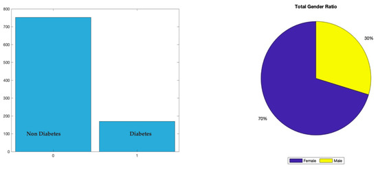
Figure 2.
Dataset distribution.
The research started by obtaining ethical approval from the Ministry of Omani Health to obtain the final dataset. Then, the prediabetic records of 920 patients from 21 polyclinics and health centres in Al Batinah South Governorate were collected. The second stage was then initiated to fill in the missing variables and features and check the data’s validity. Access to all the patient records registered under the South Al Batinah General of Health Services was granted through the Al Shifa system [35]. The researcher had to analyse every patient’s data individually and compare them with the Al Shifa system data. Any missing variables in the patient’s hard copy records were filled by utilising the patient registry in the Al Shifa system. However, if the individual’s information was missing (from the hard copy and Al Shifa system), they were recorded as an empty variable. The process of converting patient-by-patient data into an Excel file and every single hard copy into figures and tables, then verifying the data one by one through the Al Shifa system, was undertaken over six months.
Throughout these stages, there was help and support from a physician who is an expert in diabetes and had a prediabetes clinic, which was made available. Finally, a dataset of 921 Omani patients was selected to be compared with the most used PID dataset. The two datasets were created using the same approach. Table 1 presents the data collected in the prediabetes register, a record used in a dedicated clinic for a non-communicable disease screening program. Table 2 shows the diabetes mellitus scoring form, a survey completed by any patient over the age of 20 who visits a health centre for a regular check-up and is mandatory for patients over the age of 40, according to the ministry of health guidelines. The total score, as explained in Table 2, determines the diabetes risk level, i.e., if patients show a score of ≥8, they will be at a high risk of T2DM and will be examined within three months by a dedicated team that includes a diabetes doctor, nutritionist, and nurse. The patient will then usually be referred to a polyclinic or a hospital for further laboratory investigations. This process is carried out to help avoid T2DM at the earliest stage. The model has eleven clinical features (see Table 3). The data types were categorical and numerical. The register aims to enable patients with a high risk of T2DM to obtain medical aid at the earliest possible stage. Figure 2 illustrates the dataset’s total number of T2DM and non-diabetes patients. The distribution of the dataset in terms of gender was 30% male and 70% female.

Table 1.
Prediabetes register (patient data).
Table 2.
Diabetes mellitus scoring form. If the total score is <5: annual follow up. If the total score is ≥5 and <8: follow up every six months. If the total score is ≥8: follow up every three months.
Table 3.
Oman feature selections.
3.2. Variable Selection
The covariates were selected based on the Omani diagnosing DM and expert consultation system. The patient is referred to the diabetes clinic if two readings of fasting blood sugar are ≥7, which is mainly used in well-being clinics; random blood sugar ≥ 11 (which is rarely used); or two readings of HbA1C that are ≥6.5, with a time interval of 3 months. The reserved variables included age above 20, gender (two categories: male and female), and risk factors (eight categories: first-degree relative with DM). Other clinical conditions included insulin resistance, cardiovascular diseases, hypertension on therapy or BP > 140/90, HDL < 0.90 mmol/L or TAG 2.82 mmol/L, women with PCOS, physical inactivity, women with a history of GDM, body mass index, height, weight, waist circumference (cm), total cholesterol (mmol/L), and fasting plasma glucose (mmol/L) with the outcome measured as yes = 1 vs. no = 0. Figure 2 shows the total number of patients was 921, with 169 diagnosed as diabetes patients and 752 as non-diabetes patients. The Oman dataset includes all clinical tests and features found in the PID dataset except for one feature difference. In the Oman dataset, the waist circumference was used instead of the triceps skin-fold thickness. Moreover, the Oman dataset contained all genders. It has both categorical and numeric (double) predictor parameters, see Table 3.
While patients in PID dataset are all females of Pima Indian heritage at least 21 years old. All predictor parameters are numerical (double). The processed data define the PID dataset as having the following parameters:
- The total number of pregnancies;
- Glucose: a two-hour oral glucose tolerance test’s plasma glucose concentration;
- Blood Pressure: diastolic blood pressure (mm Hg);
- Skin thickness: triceps skin fold thickness (mm);
- Insulin: 2-h serum insulin (mu U/mL);
- BMI: body mass index (kg/m2);
- Diabetes pedigree function;
- Age: age (years);
- Outcome: class variable (0 or 1).
3.3. Data Processing and Cleaning
The processing data are essential for exploratory statistical analysis and further investigation of the model training phase. The more relevant data are processed, the more it would impact the feature analysis and produce a better predictive result at the time of the training data and testing. The following processes were applied:
3.3.1. Finding Missing Values from the Dataset
The Oman dataset presented in Figure 3a shows that gender has no missing value, but waist circumference and the H1bA1c have more missing values than the other categories. While processing the PID dataset, it was observed that there was no such missing data from the process see Figure 3b. Therefore, half of the operations were skipped as it had all the necessary data in the feature.

Figure 3.
Total missing values in Oman dataset and Pima Indian dataset. (a) Oman dataset, (b) Pima Indian dataset.
3.3.2. Data Pre-Processing The First Step Was for Data to Merge with Similar Categories
The data gender value was a merger of two categories {‘female’} {‘male’} instead of four categories: {‘Female’} {‘Male’}{‘female’},{‘male’}. After that, the categorial values were converted to numeric by using Group to index value, which helps to group absolute values into an index value. For gender, male is 1 and female is 2.
The second step was filling in the missing values. By using the “Ismissing” method [36], data were first analysed by running a check counter, which has missing data, i.e., (‘‘, ‘.’,’ Na’,’ NAN’), which are based on empty. The data representing these values are counted, and those particular data are selected in the row missing data, specifying which element of input data contains a missing value and the number of missing values (see Figure 4). Then, the “Fillmissing” process [37] with respect to the nearest methods was applied to each feature individually. Therefore, the NAN section is filled with the closest no-missing value.
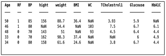
Figure 4.
Rows with missing values.
3.3.3. Exploratory Data Analysis
For the statistical operation, the data are evaluated with the individual parameter based on the categorical grouping and providing a statistical result based on the histogram. Histograms are useful for illustrating the distributional characteristics of dataset variables. It is possible to observe where the distribution peaks are, whether the distribution is symmetric or skewed, and whether there are any outliers. Histograms also help to view the possible outliers. Figure 5 and Figure 6 show a frequency distribution analysis of both datasets for features to respond for validation sent into a class of diabetic diagnosis system. Each bar covers one set of the range, and the height indicates the number of sizes in each phase range. The field of the problem we are trying to solve requires loads of related features. Since the PID dataset is an open and accessible resource, we cannot currently eliminate or generate any more data. In the dataset, we have the following features: ‘Skin Thickness’, ‘Blood Pressure, ‘Insulin’, ‘BMI’, ‘Diabetes Pedigree Function’, ‘Pregnancies’, ‘Glucose’, and ‘Age’. We may infer that ‘Skin Thickness’ is not an indication of T2DM based on a simple observation. Nevertheless, we must acknowledge that it is unusable at this point. Based on Figure 5, weight and cholesterol maximum were removed and filled with the nearest methods.

Figure 5.
Distribution analysis for Oman dataset.
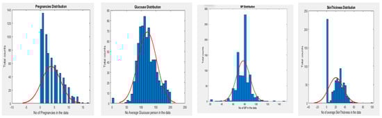

Figure 6.
Distribution analysis for PID dataset.
Another comparison is based on the boxplot. In this, the distribution of each feature is based on the outcome determined from the dataset. A box plot visualises summary statistics for sample data and can easily highlight the outliers for each parameter (see Figure 7). The box length signifies the interquartile range, and the whiskers’ sizes relative to the box’s length indicate how stretched out the rest of the values are. Thus, these aspects of the diagram provide a picture of the dispersion of the dataset. Skewness seems acceptable (<2), and it is also likely that the confidence intervals of the means are not overlapping. Therefore, a hypothesis that glucose is a measure of outcome is expected to be accurate but needs to be statistically tested. Some people have low, and some have high BP. Thus, the association between diabetes (outcome) and BP is suspect and needs to be statistically validated. Like BP, people who do not have diabetes have lower skin thickness. This is a hypothesis that has to be validated. As data of non-diabetic is skewed, diabetic samples seem to be normally distributed.
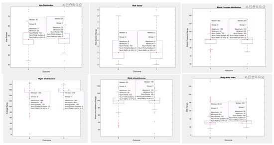

Figure 7.
Boxplot distribution for the Oman dataset based on the outcome.
3.3.4. Fill the Outlier in the Data
The outlier is a value that deviates considerably from the dataset’s general trend. Box plots are a simple way to visualise data through quantiles and identify outliers. Interquartile range (IQR) is the basic mathematics behind boxplots. The top and bottom whiskers consider the boundaries of data, and any data lying outside are outliers. The length of the box, the interquartile range, and the whiskers’ lengths relative to the box’s length give an idea of how stretched out the rest of the values are. Thus, these aspects of the diagram give a picture of the dispersion of the dataset. Skewness appears to be acceptable (<2), and it is also probable that the means’ confidence intervals do not overlap. Consequently, it is assumed that the hypothesis that glucose is a measure of outcome is valid, but it must be statistically tested. People might have low or high blood pressure. Therefore, the association between diabetes (outcome) and BP is questionable and requires statistical validation. Like those without hypertension, those without diabetes have thinner skin. This is a theory that must be validated. While non-diabetic data are skewed, diabetes samples appear to have a normal distribution. The outliers were processed using “Filloutlier” with mean and nearest method [38]. The results of outliers before and after removing both datasets’ outliers are shown in Figure 8.
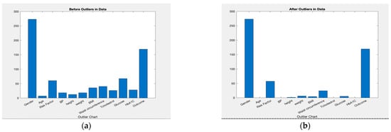

Figure 8.
Outlier processing for both datasets with and without outlier. (a) Oman; (b) Oman; (c) PID; (d) PID.
3.3.5. Data Scaling Was Applied for All Machine Learning Algorithms and ANN Using a Z-Score That Centred the Data to a Standard Deviation of 1 and a Mean of 0
The dataset’s interquartile range (IQR) describes the content of the middle 50% of values when the values are sorted. If the data median is in Q2, the median of the lower half of the data is in Q1, and the median of the upper half of the data is in Q3, then IQR = Q3−Q1 [39]. Scaling was applied for all machine learning algorithms and ANN using a z-score that centred the data to a mean of 0 and a standard deviation of 1. The dataset’s interquartile range (IQR) describes the content of the middle 50% of values when the values are sorted. If the data median is in Q2, the median of the lower half of the data is in Q1, and the median of the upper half of the data is in Q3, then IQR = Q3 − Q1 [39].
3.4. Training and Validation Datasets
Splitting the data: In order to train the datasets, there is a need to partition the data into training and testing sets. The datasets were divided with the “cvpartion” [40] function using a holdout method to split the data into two training sets: 80% training and 20% testing. For training the ANN model, datasets were divided into 80% training and 20% testing (see Table 4). We used a technique called K-fold cross-validation, which divides the dataset into K equal parts (called “folds”), then uses one of those folds as the testing set while using the combination of the other folds as the training set (see Figure 9). The model was then examined to ensure that it was accurate. The procedure repeats the processes described above K times, using a variety of folds as the testing set each time. The testing accuracy represents the procedure’s overall testing accuracy as an average.
Table 4.
Splitting the dataset.
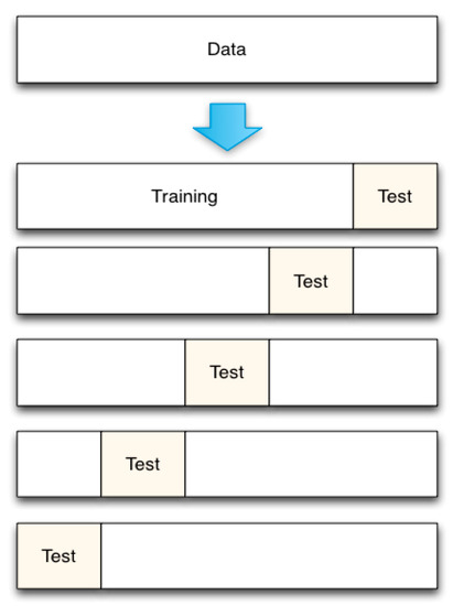
Figure 9.
K-fold C=cross-validation.
Implementation using machine learning algorithms: MATLAB (version 2021b) software command-line coding was used to create all seven models using the Oman dataset, including artificial neural networks, and the following ML algorithms were used: K-nearest neighbors, support vector machine, naive Bayes, decision tree, random forest, and linear discriminant analysis. We applied MATLAB’s “predict” function to test the model for all six machine learning models and the ANN model. A confusion matrix illustrates the predicted class correlated with the actual class, which was 0 for non-diabetes and 1 for diabetes, as shown in Figure 9 and Figure 10. The valid class presents the real data, and the predicted class delivers the performance of each algorithm in the prediction. Machine learning algorithms were used: MATLAB (version 2021b) software command-line coding was used to create all seven models using the Oman dataset, including artificial neural networks. The following ML algorithms were also used: K-nearest neighbours, support vector machine, naive Bayes, decision tree, random forest, and linear discriminant analysis. We applied MATLAB’s “predict” function to test the model for all six machine learning models and the ANN model. A confusion matrix illustrates the predicted class correlated with the actual class, which was 0 for non-diabetes and 1 for diabetes, as shown in Figure 10, Figure 11, Figure 12, Figure 13, Figure 14 and Figure 15. The valid class presents the real data, and the predicted class delivers the performance of each algorithm in the prediction.
4. Results and Discussion
Seven classification algorithms were applied to the datasets, and the results were evaluated based on accuracy, sensitivity, specificity, and precision. Generally, the outcomes were slightly different as each algorithm’s working criteria differed. The accuracy of the models was predicted with the help of a confusion matrix, as shown in Figure 4, Figure 5, Figure 6, Figure 7, Figure 8, Figure 9 and Figure 10. The results showed that the random forest and decision tree algorithms had the best classification results.
- The classification models are assessed using the metric of accuracy. Formally, accuracy is the percentage of accurate predictions made by our model. The accuracy is defined as shown below [41] and was measured in terms of positives and negatives:
- Sensitivity is a metric that evaluates a model’s ability to predict a true positive for each available category. This measure determines the proportion of positive diabetes cases predicted correctly [29]
- Specificity is the metric that evaluates a model’s ability to predict a true negative for each available category; it determines the proportion of actual negative cases predicted correctly [27].
- Precision is the proportion of true positives to all the positives; it refers to the percentage of relevant results and is a useful metric when false positives are more important than false negatives [27].
By using the equations above, the performance of the various classification models can be compared, as shown in Table 5.
Table 5.
Performance results.
4.1. Accuracy Analysis Using Confusion Matrix
4.1.1. K-Nearest Neighbours (K-NN) Is an Example of this Type of Supervised ML Algorithm
It is applicable to both classification and regression problems. K-NN classification relies on nearby feature space to classify samples. The K-NN algorithm’s default performance is illustrated in Figure 10’s confusion matrix. Of the 184 cases tested, the test identified 17 patients and 153 healthy subjects correctly. Therefore, the accuracy of the test was equal to 170 divided by 184 (92.39%).

Figure 10.
K-NN confusion matrix.
4.1.2. The Support Vector Machine (SVM) The Support Vector Machine (SVM) Works on the Margin Calculation Concept
It draws margins between the classes. The margins are removed so that the distance between the margin and the types is at a maximum and minimises the classification [42]. As illustrated in Figure 11, of the 184 cases that were tested, the test determined 29 patients and 149 healthy subjects correctly. Therefore, the accuracy of the trial was equal to 96.74%.

Figure 11.
SVM confusion matrix.
4.1.3. Naive Bayes Mainly Targets the Text Classification Industry
It is primarily used for clustering and classification purposes [43]. The underlying architecture of naive Bayes depends on conditional probability. It creates trees based on their likelihood of happening. These trees are also known as Bayesian networks. As shown in Figure 12, of the 184 cases that were tested, the test correctly determined 23 patients and 155 healthy subjects. Therefore, the accuracy of the trial was equal to 96.74%.

Figure 12.
NB confusion matrix.
4.1.4. Decision Tree (DT) Is a Supervised ML Method to Solve Classification, Prediction, and Feature Selection Problems
It aims to predict the target class based on the rules learned from the specified dataset. As a result of the 184 cases shown in Figure 13 that were tested, the test correctly determined 35 patients and 146 healthy subjects. Therefore, the accuracy of the trial was equal to 98.37%.

Figure 13.
DT confusion matrix.
4.1.5. Random Forest (RF) Is a Supervised Machine Learning Algorithm Used Widely in Classification and Regression Problems
It builds decision trees on different samples and takes their majority vote for classification and their average in case of regression. As presented in Figure 14, of the 184 subjects tested, the test correctly determined 29 patients and 152 healthy cases. Therefore, the accuracy of the test was equal to 181 divided by 184 (98.37%).

Figure 14.
RF confusion matrix.
4.1.6. Linear Discriminant Analysis Is a Statistical Technique That Can Classify Individuals into Mutually Exclusive and Exhaustive Groups Based on Independent Variables [44]
In this model, as shown in Figure 15, of the 184 cases tested, the test determined 24 patients and 153 healthy subjects correctly. Therefore, the accuracy of the trial was equal to 177 divided by 184 (96.19%).

Figure 15.
LDA confusion matrix.
4.1.7. The Conventional Artificial Neural Network (ANN) Consists of Layers and Weights
The behaviour of a network is dependent on communication between its nodes. ANN typically comprises three layers:
- Input layer: Receiving the network’s raw data input.
- Hidden layer: The functioning of a hidden layer is defined by the inputs and the weight of the connections between them and the neuron in the hidden layer. These connection weights decide whether a neuron in the hidden layer must be active or inactive.
- Output layer: The operation of this layer is determined by the outputs of the neurons in the hidden layer and the connection weight between these neurons and the neurons in the output layer.
The proposed structure of an artificial neural network, as shown in Figure 16, has an input layer with 11 features; two hidden layers, each with ten neurons; and one output layer with two outputs, diabetes and non-diabetes. A few hidden layers were used to avoid the overfitting problem because the datasets were small. A sigmoid activation function was applied to this model. It used a two-factor level function that set all input values in the values in range from 0 to 1. By using cross-entropy, the model’s performance considers the probability in a log of data points [45]. The highest accuracy achieved by this model reached 97.3%, as shown in the confusion matrix in Figure 17b, presenting the training, validation, test, and overall matrix. The accuracy achieved by the dataset’s training, validation, and testing was 97.6%, 97.4%, and 95.7%, respectively. The overall combined accuracy was 97.3%. In Figure 17d, the gradient decreased to a performance of 0.047062 and epoch number 49. This decrease means that the model was performing well up to this point, and the increase indicated the start of an overfitting problem. Another evaluation showcases the error histogram in Figure 17c, which has an error rate with a loss of the range −0.049 value. This describes the quality of the data processor and the target achieved by the evaluation.
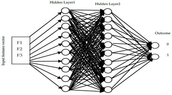
Figure 16.
ANN supervised architecture proposed.
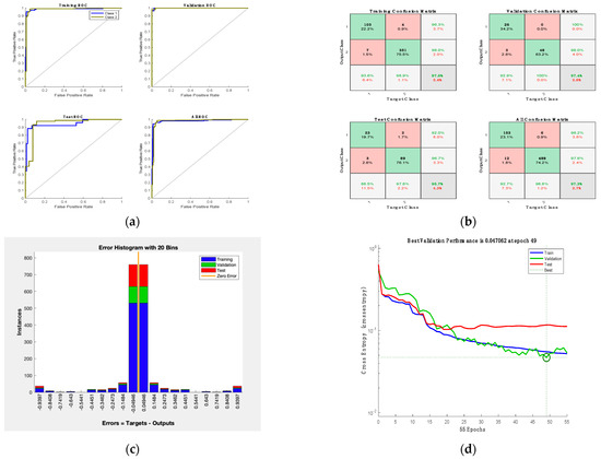
Figure 17.
ANN results: (a) receiver operation characteristic; (b) confusion matrix; (c) error histogram; (d) ANN performance.
The results of this study can be discussed, considering the results obtained from other studies. The Pima Indian Diabetes (PID) dataset (available from the University of California data repository) [16] is a dataset that has been considered in many studies. The results from similar studies were compared with our investigation and shown in Table 6.
Table 6.
Comparative performance of our proposed method against the state-of-the-art work on the same dataset.
Considering the research results on the PID dataset, the best accuracy on that data was 94% using a random forest and 88% using a decision tree [30]. In comparison, the best accuracy on our dataset was about 98.37% using two algorithms, the random forest and decision tree. One reason for the improvement in the results was the dataset used in this research, which was much larger than the PID dataset with more features. The PID dataset only has eight features and 768 cases. Furthermore, in this research, the parameters for every algorithm were optimised for the best performance. For example, in the nearest neighbours method, the parameter k varied between one and five to find the most optimised method. Moreover, in choosing the parameters for the artificial neural network, the number of hidden layer neurons and the accuracy of the network were strongly correlated, which meant that for various neurons, the network was resolved to find the best accuracy. Finally, the optimised number of neurons with the highest accuracy was chosen. The comparison with similar studies which use the most used diabetes dataset, the PID dataset, and the classification approaches are presented in Table 6.
All of the models in Table 7 were applied utilising two different feature sets. The first feature set contained eight clinical characteristics that were the same as those on PID, and the second feature set contained eleven additional clinical characteristics that were based on the Oman diagnostic method. A comparison was made between the PID models and the accuracy outcomes. According to the findings, increasing the number of features in a model improves its classification accuracy. The results show an accuracy ranging from 92.39 to 98.37%, which is higher than in Table 6. Training outcomes for all models across all datasets in terms of time and speed are displayed in Table 8.
Table 7.
Performance evaluation of the proposed method on both datasets.
Table 8.
Comparison of time complexity and models training speed.
While training the model, none of the features were utilised by the trainer due to the following reason. The drop in score between the first and second most essential predictors is significant, while the drops after the sixth predictor are relatively small. A reduction in the critical score represents confidence in feature selection. Therefore, the significant drop implies that the software is confident in selecting the most important predictor. The small reductions indicate that the difference in predictor importance is not significant. The top five most important predictors were selected, as shown in Figure 18. The possibilities for the diabetic prediction from Oman were based on HbA1c and glucose values, and the prospects for the diabetic forecasts from PID were based on the glucose values. These features hold more weightage for the feature processing and have important scores to reproduce the probability of the feature selections.
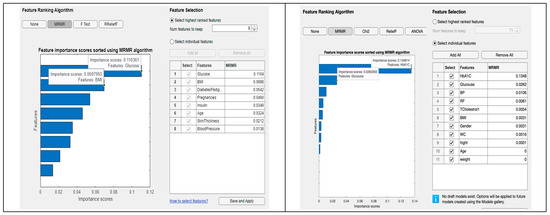
Figure 18.
Comparative performance of our proposed method in both datasets.
5. Conclusions
This paper proposes a method to discriminate between patients affected by diabetes and those not affected by using machine-learning algorithms and artificial neural networks. We evaluated our approach using real-world data extracted from the Omani well-being program. We then compared it with a widely used dataset by researchers, the Pima Indian Diabetes dataset, which describes a population near Phoenix, Arizona. Training the model using seven different classification algorithms, we obtained the equal highest accuracy with random forest and decision tree with an accuracy of 98.37%. The proposed model shows significant performance in selecting the most accurate predictors of diabetes. In the future, it would be intriguing to see the classification of additional types of medical data under this framework, thereby providing a cost-effective and time-saving option for diabetic patients and physicians. More attributes can boost performance and provide more accurate forecasts. Moreover, feature selection techniques can be explored.
Author Contributions
Originality of dataset, K.A.S.; Conceptualisation, K.A.S. and W.B.; software, K.A.S.; validation, K.A.S.; data curation, K.A.S.; visualisation, K.A.S.; supervision, W.B.; writing, K.A.S. and W.B.; writing—original draft preparation, K.A.S. All authors have read and agreed to the published version of the manuscript.
Funding
This research received no external funding.
Institutional Review Board Statement
This study was approved by the Research and Ethical Review & Approval Committee, Ministry of Health, Oman (Proposal ID: MoH/CSW20/24055, 23/122020). This study does not involve humans or animals.
Informed Consent Statement
Not applicable.This study did not involve humans.
Data Availability Statement
The Espcialy created Omani Prediabetes dataset that support the findings of this study can be available from the corresponding author upon reasonable request. Pima Indian dataset can be found here: https://www.kaggle.com/kumargh/pimaindiansdiabetescsv (accessed on 15 November 2021).
Conflicts of Interest
The authors declare no conflict of interest.
References
- World Health Organization. Noncommunicable Diseases (NCD) Country Profiles. 2018. Available online: https://www.who.int/nmh/countries/omn_en.pdf (accessed on 15 November 2021).
- Peters, S.A.; Huxley, R.R.; Woodward, M. Diabetes as a risk factor for stroke in women compared with men: A systematic review and meta-analysis of 64 cohorts, including 775,385 individuals and 12,539 strokes. Lancet 2014, 383, 19731980. [Google Scholar] [CrossRef] [PubMed]
- Vos, T.; Lim, S.S.; Abbiati, C.; Abbas, K.M.; Abbasi, M.; Abbasifard, M.; Abbasi-Kangevari, M.; Abbastabar, H.; Abd-Allah, F.; Abdelalim, A.; et al. Global burden of 369 diseases and injuries in 204 countries and territories, 1990–2019: A systematic analysis for the Global Burden of Disease Study 2019. Lancet 2020, 396, 1204–1222. [Google Scholar] [CrossRef] [PubMed]
- Aljulifi, M.Z. Prevalence and reasons of increased type 2 diabetes in Gulf Cooperation Council Countries. Saudi Med. J. 2021, 42, 481–490. [Google Scholar] [CrossRef] [PubMed]
- Sarwar, A.; Sharma, V. Comparative analysis of machine learning techniques in prognosis of type II diabetes. AI Soc. 2014, 29, 123–129. [Google Scholar] [CrossRef]
- Kumari, V.A.; Chitra, R. Classification of diabetes disease using support vector machine. Int. J. Adv. Comput. Sci. Appl. 2013, 3, 1797–1801. [Google Scholar]
- Negi, A.; Jaiswal, V. A First Attempt to Develop a Diabetes Prediction Method Based on Different Global Datasets. In Proceedings of the 2016 Fourth International Conference on Parallel, Distributed and Grid Computing (PDGC), Waknaghat, India, 22–24 December 2016; pp. 237–241. [Google Scholar]
- Maniruzzaman, M.; Kumar, N.; Menhazul Abedin, M.; Shaykhul Islam, M.; Suri, H.S.; El-Baz, A.S.; Suri, J.S. Comparative approaches for classification of diabetes mellitus data: Machine learning paradigm. Comput. Methods Programs Biomed. 2017, 152, 23–34. [Google Scholar] [CrossRef]
- Olaniyi, E.O.; Adnan, K. Onset diabetes diagnosis using artificial neural network. Int. J. Sci. Eng. Res. 2014, 5, 754–759. [Google Scholar]
- Wei, S.; Zhao, X.; Miao, C. A comprehensive exploration to the machine learning techniques for diabetes identification. In Proceedings of the 2018 IEEE 4th World Forum on Internet of Things (WF-IoT), Singapore, 5–8 February 2018. [Google Scholar] [CrossRef]
- Anwar, F.; Qurat-Ul-Ain, F.A.; Ejaz, M.Y.; Mosavi, A. A comparative analysis on diagnosis of diabetes mellitus using different approaches—A survey. Inform. Med. Unlocked 2020, 21, 100482. [Google Scholar] [CrossRef]
- Swapna, G.; Vinayakumar, R.; Soman, K.P. Diabetes detection using deep learning algorithms. ICT Express 2018, 4, 243–246. [Google Scholar]
- Chaves, L.; Marques, G. Data Mining Techniques for Early Diagnosis of Diabetes: A Comparative Study. Appl. Sci. 2021, 11, 2218. [Google Scholar] [CrossRef]
- Grądalski, T.; Hołoń, A. Diabetes mellitus in the last weeks of life—Case study and current literature review. Med. Paliatywna 2019, 11, 67–72. [Google Scholar] [CrossRef]
- Mirshahvalad, R.; Zanjani, N.A. Diabetes prediction using the ensemble perceptron algorithm. In Proceedings of the 2017 9th International Conference on Computational Intelligence and Communication Networks (CICN), Girne, Cyprus, 16–17 September 2017; pp. 190–194. [Google Scholar]
- Kumar. Pima-Indians-Diabetes.csv. Kaggle. 2018. Available online: https://www.kaggle.com/kumargh/pimaindiansdiabetescsv (accessed on 18 June 2021).
- Perveen, S.; Shahbaz, M.; Guergachi, A.; Keshavjee, K. Performance analysis of data mining classification techniques to predict diabetes. Procedia Comput. Sci. 2016, 82, 115–121. [Google Scholar] [CrossRef]
- Khan, N.S.; Muaz, M.H.; Kabir, A.; Islam, M.N. A machine learning-based intelligent system for predicting diabetes. Int. J. Big Data Anal. Healthc. 2019, 4, 20. [Google Scholar] [CrossRef]
- Nai-Arun, N.; Moungmai, R. Comparison of classifiers for the risk of diabetes prediction. Procedia Comput. Sci. 2015, 69, 132–142. [Google Scholar] [CrossRef]
- Kocher, T.; Holtfreter, B.; Petersmann, A.; Eickholz, P.; Hoffmann, T.; Kaner, D.; Kim, T.; Meyle, J.; Schlagenhauf, U.; Doering, S.; et al. Effect of periodontal treatment on HbA1c among patients with prediabetes. J. Dent. Res. 2019, 98, 171–179. [Google Scholar] [CrossRef] [PubMed]
- Meng, X.H.; Huang, Y.X.; Rao, D.P.; Zhang, Q.; Liu, Q. Comparison of three data mining models for predicting diabetes or prediabetes by risk factors. Kaohsiung J. Med. Sci. 2013, 29, 93–99. [Google Scholar] [CrossRef]
- Sheikhi, G.; Altınçay, H. The cost of type II diabetes mellitus: A machine learning perspective. In IFMBE Proceedings, Proceedings of the XIV Mediterranean Conference on Medical and Biological Engineering and Computing, Paphos, Cyprus, 31 March–2 April 2016; Kyriacou, E., Christofides, S., Pattichis, C.S., Eds.; Springer: Cham, Switzerland, 2016; Volume 57, pp. 818–821. [Google Scholar] [CrossRef]
- Iyer, A.; Jeyalatha, S.; Sumbaly, R. Diagnosis of diabetes using classification mining techniques. Int. J. Data Min. Knowl. Manag. Process 2015, 5, 1–14. [Google Scholar] [CrossRef]
- Barik, S.; Mohanty, S.; Mohanty, S.; Singh, D. Analysis of Prediction Accuracy of Diabetes Using Classifier and Hybrid Machine Learning Techniques. In Intelligent and Cloud Computing. Smart Innovation, Systems and Technologies; Mishra, D., Buyya, R., Mohapatra, P., Patnaik, S., Eds.; Springer: Singapore, 2021; Volume 153, pp. 399–409. [Google Scholar] [CrossRef]
- Ephzibah, E.P. A hybrid genetic-fuzzy expert system for effective heart disease diagnosis. In Communications in Computer and Information Science, Proceedings of the Advances in Computing and Information Technology, First International Conference, ACITY 2011, Chennai, India, 15–17 July 2011; Wyld, D.C., Wozniak, M., Chaki, N., Meghanathan, N., Nagamalai, D., Eds.; Springer: Berlin/Heidelberg, Germany, 2011; Volume 198, pp. 115–121. [Google Scholar] [CrossRef]
- Zheng, T.; Xie, W.; Xu, L.L.; He, X.Y.; Zhang, Y.; You, M.R.; Yang, G.; Chen, Y. A machine learning-based framework to identify type 2 diabetes through electronic health records. Int. J. Med. Inform. 2017, 97, 120–127. [Google Scholar] [CrossRef]
- Zou, Q.; Qu, K.Y.; Luo, Y.M.; Yin, D.H.; Ju, Y.; Tang, H. Predicting diabetes mellitus with machine learning techniques. Front. Genet. 2018, 9, 515. [Google Scholar] [CrossRef] [PubMed]
- Malik, S.; Khadgawat, R.; Anand, S.; Gupta, S. Non-invasive detection of fasting blood glucose level via electrochemical measurement of saliva. SpringerPlus 2016, 5, 701. [Google Scholar] [CrossRef]
- Lekha, S.; Suchetha, M. Real-Time Non-Invasive Detection and Classification of Diabetes Using Modified Convolution Neural Network. IEEE J. Biomed. Health Inform. 2018, 22, 1630–1636. [Google Scholar] [CrossRef] [PubMed]
- Yuvaraj, N.; Sri Preethaa, K.R. Diabetes prediction in healthcare systems using machine learning algorithms on Hadoop cluster. Clust. Comput. 2019, 22, 1–9. [Google Scholar] [CrossRef]
- Sisodia, D.; Sisodia, D.S. Prediction of Diabetes using Classification Algorithms. Procedia Comput. Sci. 2018, 132, 1578–1585. [Google Scholar] [CrossRef]
- Mercaldo, F.; Nardone, V.; Santone, A. Diabetes Mellitus Affected Patients Classification and Diagnosis through Machine Learning Techniques. Procedia Comput. Sci. 2017, 112, 2519–2528. [Google Scholar] [CrossRef]
- Maniruzzaman, M.; Rahman, M.J.; Ahammed, B.; Abedin, M.M. Classification and prediction of diabetes disease using machine learning paradigm. Health Inf. Sci. Syst. 2020, 8, 7. [Google Scholar] [CrossRef] [PubMed]
- Saberi-Movahed, F.; Rostami, M.; Berahmand, K.; Karami, S.; Tiwari, P.; Oussalah, M.; Band, S.S. Dual Regularized Unsupervised Feature Selection Based on Matrix Factorization and Minimum Redundancy with application in gene selection. Knowl.-Based Syst. 2022, 256, 109884. [Google Scholar] [CrossRef]
- Ministry of Health Al Shifa System. (n.d.). Available online: https://omanportal.gov.om/wps/wcm/connect/2a19ffae-ade0-428b-9f7c-b30bdd874882/Al%2BShifa_MoH.pdf?MOD=AJPERES (accessed on 29 July 2021).
- Find Missing Values—MATLAB. 2022. Available online: https://www.mathworks.com/help/matlab/ref/ismissing.html?s_tid=doc_ta. (accessed on 29 July 2021).
- Fill Missing Values—MATLAB. 2022. Available online: https://www.mathworks.com/help/matlab/ref/fillmissing.html?s_tid=doc_ta (accessed on 29 July 2021).
- Detect and Replace Outliers in Data—MATLAB. Available online: https://www.mathworks.com/help/matlab/ref/filloutliers.html?s_tid=doc_ta (accessed on 30 August 2022).
- Partition Data for Cross-Validation—MATLAB. Available online: https://www.mathworks.com/help/stats/cvpartition.html (accessed on 9 August 2021).
- Mathworks. Normalise Data—MATLAB Normalize. Available online: https://www.mathworks.com/help/matlab/ref/double.normalize.html (accessed on 28 March 2022).
- Lador, S.M. What Metrics Should Be Used for Evaluating a Model on an Imbalanced Data Set? Medium, 22 October 2017. Available online: https://towardsdatascience.com/what-metrics-should-we-use-on-imbalanced-data-set-precision-recall-roc-e2e79252aeba (accessed on 27 June 2022).
- Lavrac, N.; Keravnou, E.; Zupan, B. Intelligent Data Analysis in Medicine. In Encyclopedia of Computer Science and Technology; Dekker: New York, NY, USA, 2000; Volume 42. [Google Scholar]
- Lowd, D.; Domingos, P. Naive Bayes Models for Probability Estimation. In Proceedings of the 22nd International Conference on Machine Learning, Bonn, Germany, 7–11 August 2005; Available online: https://dl.acm.org/doi/abs/10.1145/1102351.1102418?casa_token=93gP6KZPvIEAAAAA%3AR7o8Y2erGyVaOKEtyDCVmLZLu_Kth5VcLyihYXQ9A0tiFR7eEYRelyjwHAsdpNqnho34tEdNnnk (accessed on 15 May 2021).
- Performance for Diabetes with Linear Discriminant Analysis and Genetic Algorithm. Available online: https://ieeexplore.ieee.org/stamp/stamp.jsp?tp=&arnumber=9637039 (accessed on 25 January 2022).
- Mathworks. Cross-Entropy Loss for Classification Tasks—MATLAB Crossentropy. Available online: https://www.mathworks.com/help/deeplearning/ref/dlarray.crossentropy.html (accessed on 28 January 2022).
Disclaimer/Publisher’s Note: The statements, opinions and data contained in all publications are solely those of the individual author(s) and contributor(s) and not of MDPI and/or the editor(s). MDPI and/or the editor(s) disclaim responsibility for any injury to people or property resulting from any ideas, methods, instructions or products referred to in the content. |
© 2023 by the authors. Licensee MDPI, Basel, Switzerland. This article is an open access article distributed under the terms and conditions of the Creative Commons Attribution (CC BY) license (https://creativecommons.org/licenses/by/4.0/).